
Exploring Entanglement Spectra and Phase Diagrams in Multi-Electron Quantum Dot Chains


Abstract
1. Introduction
2. Extended Hubbard Model
3. Reduced Density Matrices and Entanglement
3.1. Local Entanglement of Multi-Electron Quantum Dot
3.2. Pairwise Entanglement of Multi-Electron Quantum Dot
4. Results
4.1. Local Entanglement at
4.2. Pairwise Entanglement at
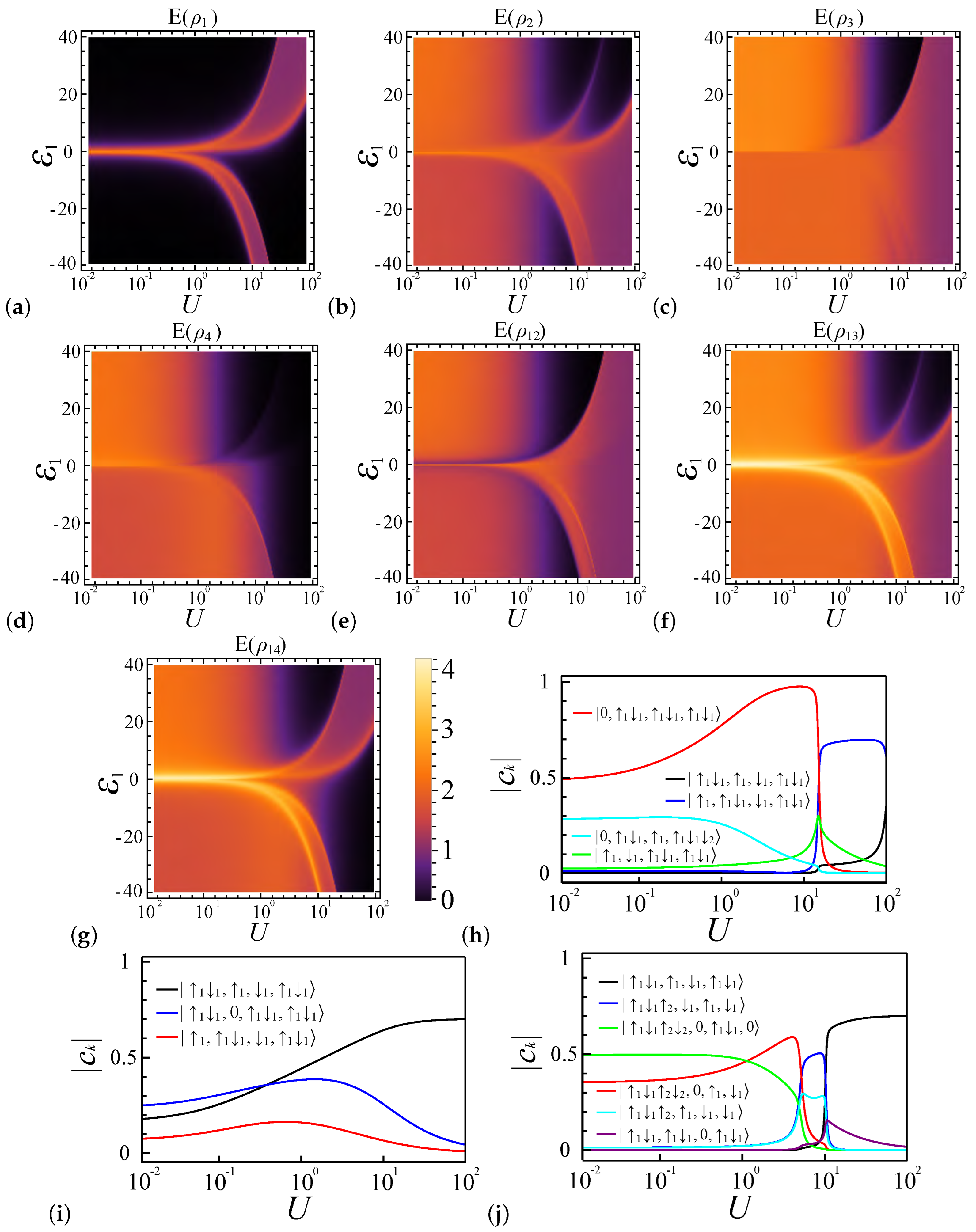
4.3. Entanglement Analysis for with
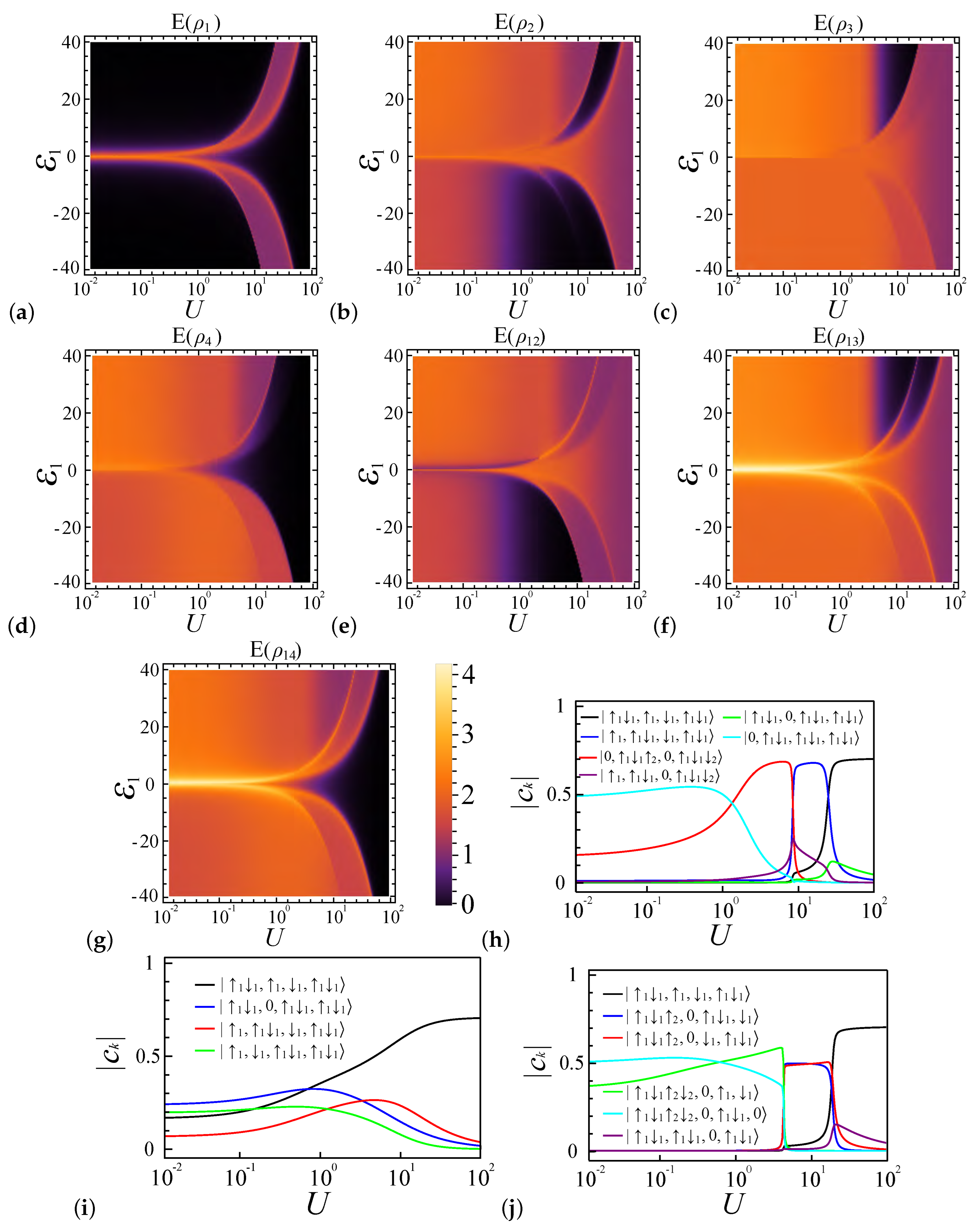
4.4. Entanglement Analysis for with
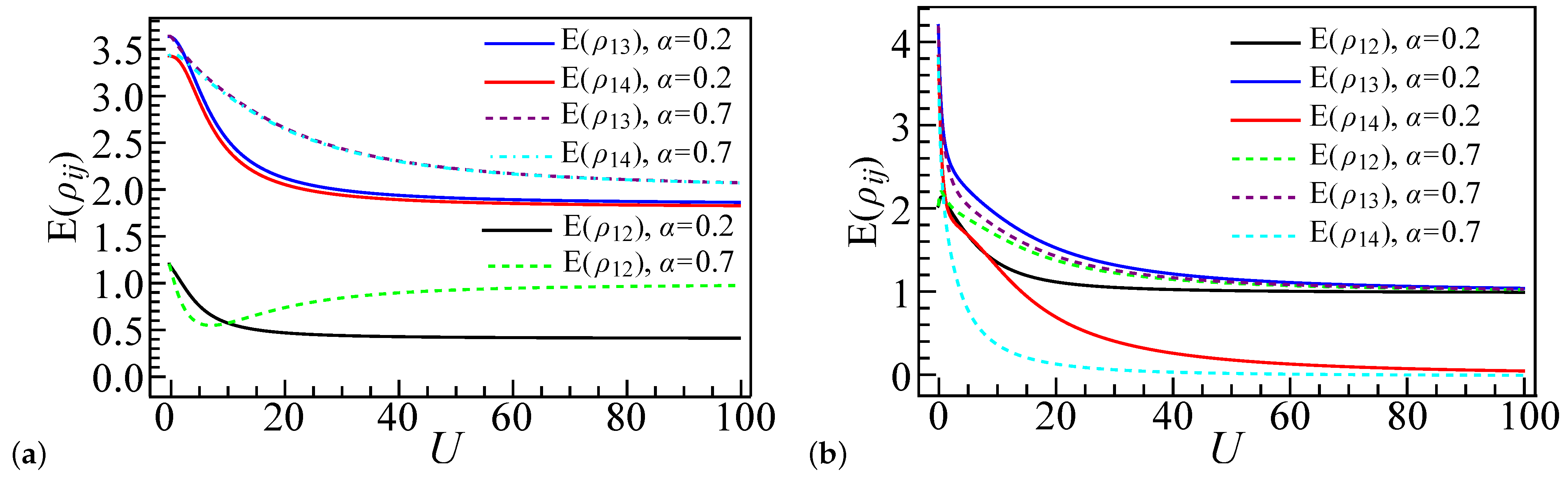
4.5. Entanglement Comparison for Larger Systems
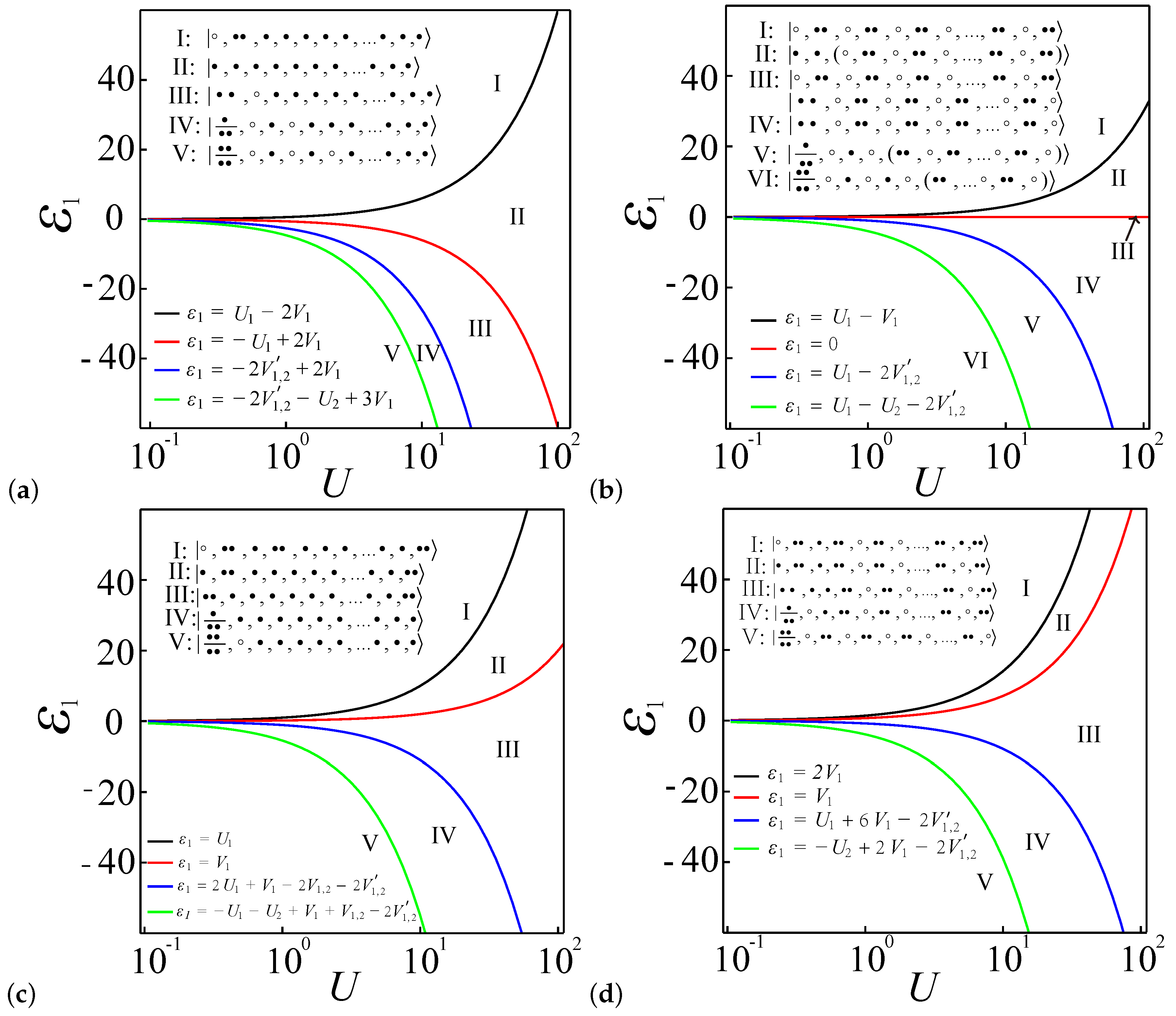
4.6. Boundaries of Entanglement Diagrams for Large Systems
5. Conclusions
Author Contributions
Funding
Institutional Review Board Statement
Data Availability Statement
Acknowledgments
Conflicts of Interest
References
- Braunstein, S.L.; van Loock, P. Quantum information with continuous variables. Rev. Mod. Phys. 2005, 77, 513–577. [Google Scholar] [CrossRef]
- Abaach, S.; Mzaouali, Z.; El Baz, M. Long distance entanglement and high-dimensional quantum teleportation in the Fermi–Hubbard model. Sci. Rep. 2023, 13, 964. [Google Scholar] [CrossRef] [PubMed]
- Amico, L.; Fazio, R.; Osterloh, A.; Vedral, V. Entanglement in many-body systems. Rev. Mod. Phys. 2008, 80, 517–576. [Google Scholar] [CrossRef]
- Schulz, M.; Hooley, C.A.; Moessner, R.; Pollmann, F. Stark Many-Body Localization. Phys. Rev. Lett. 2019, 122, 040606. [Google Scholar] [CrossRef]
- Iyer, S.; Oganesyan, V.; Refael, G.; Huse, D.A. Many-body localization in a quasiperiodic system. Phys. Rev. B 2013, 87, 134202. [Google Scholar] [CrossRef]
- Pal, A.; Huse, D.A. Many-body localization phase transition. Phys. Rev. B 2010, 82, 174411. [Google Scholar] [CrossRef]
- Bugu, S.; Ozaydin, F.; Ferrus, T.; Kodera, T. Preparing Multipartite Entangled Spin Qubits via Pauli Spin Blockade. Sci. Rep. 2020, 10, 3481. [Google Scholar] [CrossRef]
- Fedele, F.; Chatterjee, A.; Fallahi, S.; Gardner, G.C.; Manfra, M.J.; Kuemmeth, F. Simultaneous Operations in a Two-Dimensional Array of Singlet-Triplet Qubits. PRX Quantum 2021, 2, 040306. [Google Scholar] [CrossRef]
- Gonzalez-Zalba, M.F.; de Franceschi, S.; Charbon, E.; Meunier, T.; Vinet, M.; Dzurak, A.S. Scaling silicon-based quantum computing using CMOS technology. Nat. Electron. 2021, 4, 872–884. [Google Scholar] [CrossRef]
- Philips, S.G.J.; Madzik, M.T.; Amitonov, S.V.; de Snoo, S.L.; Russ, M.; Kalhor, N.; Volk, C.; Lawrie, W.I.L.; Brousse, D.; Tryputen, L.; et al. Universal control of a six-qubit quantum processor in silicon. Nature 2022, 609, 919–924. [Google Scholar] [CrossRef]
- Zwolak, J.P.; Taylor, J.M. Colloquium: Advances in automation of quantum dot devices control. Rev. Mod. Phys. 2023, 95, 011006. [Google Scholar] [CrossRef] [PubMed]
- Reed, M.D.; Maune, B.M.; Andrews, R.W.; Borselli, M.G.; Eng, K.; Jura, M.P.; Kiselev, A.A.; Ladd, T.D.; Merkel, S.T.; Milosavljevic, I.; et al. Reduced Sensitivity to Charge Noise in Semiconductor Spin Qubits via Symmetric Operation. Phys. Rev. Lett. 2016, 116, 110402. [Google Scholar] [CrossRef] [PubMed]
- Feng, M.; Zaw, L.H.; Koh, T.S. Two-qubit sweet spots for capacitively coupled exchange-only spin qubits. NPJ Quantum Inf. 2021, 7, 112. [Google Scholar] [CrossRef]
- Feng, M.; Yoneda, J.; Huang, W.; Su, Y.; Tanttu, T.; Yang, C.H.; Cifuentes, J.D.; Chan, K.W.; Gilbert, W.; Leon, R.C.C.; et al. Control of dephasing in spin qubits during coherent transport in silicon. Phys. Rev. B 2023, 107, 085427. [Google Scholar] [CrossRef]
- Shi, Z.; Simmons, C.B.; Prance, J.R.; Gamble, J.K.; Koh, T.S.; Shim, Y.P.; Hu, X.; Savage, D.E.; Lagally, M.G.; Eriksson, M.A.; et al. Fast Hybrid Silicon Double-Quantum-Dot Qubit. Phys. Rev. Lett. 2012, 108, 140503. [Google Scholar] [CrossRef]
- Teitelboim, A.; Meir, N.; Kazes, M.; Oron, D. Colloidal Double Quantum Dots. Acc. Chem. Res. 2016, 49, 902–910. [Google Scholar] [CrossRef]
- Hensgens, T.; Fujita, T.; Janssen, L.; Li, X.; Van Diepen, C.J.; Reichl, C.; Wegscheider, W.; Das Sarma, S.; Vandersypen, L.M.K. Quantum simulation of a Fermi–Hubbard model using a semiconductor quantum dot array. Nature 2017, 548, 70. [Google Scholar] [CrossRef]
- van Diepen, C.J.; Hsiao, T.K.; Mukhopadhyay, U.; Reichl, C.; Wegscheider, W.; Vandersypen, L.M.K. Quantum Simulation of Antiferromagnetic Heisenberg Chain with Gate-Defined Quantum Dots. Phys. Rev. X 2021, 11, 041025. [Google Scholar] [CrossRef]
- Buterakos, D.; Das Sarma, S. Certain exact many-body results for Hubbard model ground states testable in small quantum dot arrays. Phys. Rev. B 2023, 107, 014403. [Google Scholar] [CrossRef]
- Dehollain, J.P.; Mukhopadhyay, U.; Michal, V.P.; Wang, Y.; Wunsch, B.; Reichl, C.; Wegscheider, W.; Rudner, M.S.; Demler, E.; Vandersypen, L.M.K. Nagaoka ferromagnetism observed in a quantum dot plaquette. Nature 2020, 579, 528–533. [Google Scholar] [CrossRef]
- Kiczynski, M.; Gorman, S.K.; Geng, H.; Donnelly, M.B.; Chung, Y.; He, Y.; Keizer, J.G.; Simmons, M.Y. Engineering topological states in atom-based semiconductor quantum dots. Nature 2022, 606, 694–699. [Google Scholar] [CrossRef] [PubMed]
- Wang, X.; Khatami, E.; Fei, F.; Wyrick, J.; Namboodiri, P.; Kashid, R.; Rigosi, A.F.; Bryant, G.; Silver, R. Experimental realization of an extended Fermi-Hubbard model using a 2D lattice of dopant-based quantum dots. Nat. Commun. 2022, 13, 6824. [Google Scholar] [CrossRef] [PubMed]
- Le, N.H.; Fisher, A.J.; Curson, N.J.; Ginossar, E. Topological phases of a dimerized Fermi–Hubbard model for semiconductor nano-lattices. NPJ Quantum Inf. 2020, 6, 24. [Google Scholar] [CrossRef]
- Wang, X.; Yang, S.; Das Sarma, S. Quantum theory of the charge-stability diagram of semiconductor double-quantum-dot systems. Phys. Rev. B 2011, 84, 115301. [Google Scholar] [CrossRef]
- Das Sarma, S.; Wang, X.; Yang, S. Hubbard model description of silicon spin qubits: Charge stability diagram and tunnel coupling in Si double quantum dots. Phys. Rev. B 2011, 83, 235314. [Google Scholar] [CrossRef]
- Yang, S.; Wang, X.; Das Sarma, S. Generic Hubbard model description of semiconductor quantum-dot spin qubits. Phys. Rev. B 2011, 83, 161301. [Google Scholar] [CrossRef]
- Watson, T.F.; Philips, S.G.J.; Kawakami, E.; Ward, D.R.; Scarlino, P.; Veldhorst, M.; Savage, D.E.; Lagally, M.G.; Friesen, M.; Coppersmith, S.N.; et al. A programmable two-qubit quantum processor in silicon. Nature 2018, 555, 633–637. [Google Scholar] [CrossRef]
- Zieliński, M. Double nanowire quantum dots and machine learning. Sci. Rep. 2025, 15, 5939. [Google Scholar] [CrossRef]
- Hosseiny, S.M. Quantum dense coding and teleportation based on two coupled quantum dot molecules influenced by intrinsic decoherence, tunneling rates, and Coulomb coupling interaction. Appl. Phys. B 2023, 130, 8. [Google Scholar] [CrossRef]
- Bugu, S.; Ozaydin, F.; Kodera, T. Surpassing the classical limit in magic square game with distant quantum dots coupled to optical cavities. Sci. Rep. 2020, 10, 22202. [Google Scholar] [CrossRef]
- Ferreira, M.; Rojas, O.; Rojas, M. Thermal entanglement and quantum coherence of a single electron in a double quantum dot with Rashba interaction. Phys. Rev. A 2023, 107, 052408. [Google Scholar] [CrossRef]
- Dahbi, Z.; Oumennana, M.; El Anouz, K.; Mansour, M.; El Allati, A. Quantum Fisher information versus quantum skew information in double quantum dots with Rashba interaction. Appl. Phys. B 2023, 129, 27. [Google Scholar] [CrossRef]
- Zajac, D.M.; Sigillito, A.J.; Russ, M.; Borjans, F.; Taylor, J.M.; Burkard, G.; Petta, J.R. Resonantly driven CNOT gate for electron spins. Science 2018, 359, 439. [Google Scholar] [CrossRef] [PubMed]
- Cerfontaine, P.; Botzem, T.; Ritzmann, J.; Humpohl, S.S.; Ludwig, A.; Schuh, D.; Bougeard, D.; Wieck, A.D.; Bluhm, H. Closed-loop control of a GaAs-based singlet-triplet spin qubit with 99.5% gate fidelity and low leakage. Nat. Commun. 2020, 11, 4144. [Google Scholar] [CrossRef]
- Martins, F.; Malinowski, F.K.; Nissen, P.D.; Barnes, E.; Fallahi, S.; Gardner, G.C.; Manfra, M.J.; Marcus, C.M.; Kuemmeth, F. Noise Suppression Using Symmetric Exchange Gates in Spin Qubits. Phys. Rev. Lett. 2016, 116, 116801. [Google Scholar] [CrossRef]
- Loss, D.; DiVincenzo, D.P. Quantum computation with quantum dots. Phys. Rev. A 1998, 57, 120–126. [Google Scholar] [CrossRef]
- Burkard, G.; Loss, D.; DiVincenzo, D.P. Coupled quantum dots as quantum gates. Phys. Rev. B 1999, 59, 2070–2078. [Google Scholar] [CrossRef]
- Baruffa, F.; Stano, P.; Fabian, J. Spin-orbit coupling and anisotropic exchange in two-electron double quantum dots. Phys. Rev. B 2010, 82, 045311. [Google Scholar] [CrossRef]
- Maune, B.M.; Borselli, M.G.; Huang, B.; Ladd, T.D.; Deelman, P.W.; Holabird, K.S.; Kiselev, A.A.; Alvarado-Rodriguez, I.; Ross, R.S.; Schmitz, A.E.; et al. Coherent singlet-triplet oscillations in a silicon-based double quantum dot. Nature 2012, 481, 344–347. [Google Scholar] [CrossRef]
- Mehl, S.; DiVincenzo, D.P. Inverted singlet-triplet qubit coded on a two-electron double quantum dot. Phys. Rev. B 2014, 90, 195424. [Google Scholar] [CrossRef]
- Martins, F.; Malinowski, F.K.; Nissen, P.D.; Fallahi, S.; Gardner, G.C.; Manfra, M.J.; Marcus, C.M.; Kuemmeth, F. Negative Spin Exchange in a Multielectron Quantum Dot. Phys. Rev. Lett. 2017, 119, 227701. [Google Scholar] [CrossRef] [PubMed]
- Malinowski, F.K.; Martins, F.; Smith, T.B.; Bartlett, S.D.; Doherty, A.C.; Nissen, P.D.; Fallahi, S.; Gardner, G.C.; Manfra, M.J.; Marcus, C.M.; et al. Spin of a Multielectron Quantum Dot and Its Interaction with a Neighboring Electron. Phys. Rev. X 2018, 8, 011045. [Google Scholar] [CrossRef]
- Barnes, E.; Kestner, J.P.; Nguyen, N.T.T.; Das Sarma, S. Screening of charged impurities with multielectron singlet-triplet spin qubits in quantum dots. Phys. Rev. B 2011, 84, 235309. [Google Scholar] [CrossRef]
- Srinivasa, V.; Xu, H.; Taylor, J.M. Tunable Spin-Qubit Coupling Mediated by a Multielectron Quantum Dot. Phys. Rev. Lett. 2015, 114, 226803. [Google Scholar] [CrossRef] [PubMed]
- Leon, R.C.C.; Yang, C.H.; Hwang, J.C.C.; Camirand Lemyre, J.; Tanttu, T.; Huang, W.; Huang, J.Y.; Hudson, F.E.; Itoh, K.M.; Laucht, A.; et al. Bell-state tomography in a silicon many-electron artificial molecule. Nat. Commun. 2021, 12, 3228. [Google Scholar] [CrossRef]
- Potts, H.; Josefi, J.; Chen, I.J.; Lehmann, S.; Dick, K.A.; Leijnse, M.; Reimann, S.M.; Bengtsson, J.; Thelander, C. Symmetry-controlled singlet-triplet transition in a double-barrier quantum ring. Phys. Rev. B 2021, 104, L081409. [Google Scholar] [CrossRef]
- Kiyama, H.; Yoshimi, K.; Kato, T.; Nakajima, T.; Oiwa, A.; Tarucha, S. Preparation and Readout of Multielectron High-Spin States in a Gate-Defined GaAs/AlGaAs Quantum Dot. Phys. Rev. Lett. 2021, 127, 086802. [Google Scholar] [CrossRef]
- Higginbotham, A.P.; Kuemmeth, F.; Hanson, M.P.; Gossard, A.C.; Marcus, C.M. Coherent Operations and Screening in Multielectron Spin Qubits. Phys. Rev. Lett. 2014, 112, 026801. [Google Scholar] [CrossRef]
- Deng, K.; Calderon-Vargas, F.A.; Mayhall, N.J.; Barnes, E. Negative exchange interactions in coupled few-electron quantum dots. Phys. Rev. B 2018, 97, 245301. [Google Scholar] [CrossRef]
- Chan, G.X.; Wang, X. Microscopic theory of a magnetic-field-tuned sweet spot of exchange interactions in multielectron quantum-dot systems. Phys. Rev. B 2022, 105, 245409. [Google Scholar] [CrossRef]
- Hu, X.; Das Sarma, S. Spin-based quantum computation in multielectron quantum dots. Phys. Rev. A 2001, 64, 042312. [Google Scholar] [CrossRef]
- Ercan, H.E.; Anderson, C.R.; Coppersmith, S.N.; Friesen, M.; Gyure, M.F. Multielectron dots provide faster Rabi oscillations when the core electrons are strongly confined. arXiv 2023, arXiv:2303.02958. [Google Scholar]
- Chan, G.X.; Wang, X. Robust entangling gate for capacitively coupled few-electron singlet-triplet qubits. Phys. Rev. B 2022, 106, 075417. [Google Scholar] [CrossRef]
- Malinowski, F.K.; Martins, F.; Smith, T.B.; Bartlett, S.D.; Doherty, A.C.; Nissen, P.D.; Fallahi, S.; Gardner, G.C.; Manfra, M.J.; Marcus, C.M.; et al. Fast spin exchange across a multielectron mediator. Nat. Commun. 2019, 10, 1196. [Google Scholar] [CrossRef]
- Deng, K.; Barnes, E. Interplay of exchange and superexchange in triple quantum dots. Phys. Rev. B 2020, 102, 035427. [Google Scholar] [CrossRef]
- Chan, G.X.; Wang, X. Sign switching of superexchange mediated by a few electrons in a nonuniform magnetic field. Phys. Rev. A 2022, 106, 022420. [Google Scholar] [CrossRef]
- Qiao, H.; Kandel, Y.P.; Fallahi, S.; Gardner, G.C.; Manfra, M.J.; Hu, X.; Nichol, J.M. Long-Distance Superexchange between Semiconductor Quantum-Dot Electron Spins. Phys. Rev. Lett. 2021, 126, 017701. [Google Scholar] [CrossRef]
- Bakker, M.A.; Mehl, S.; Hiltunen, T.; Harju, A.; DiVincenzo, D.P. Validity of the single-particle description and charge noise resilience for multielectron quantum dots. Phys. Rev. B 2015, 91, 155425. [Google Scholar] [CrossRef]
- Mehl, S.; DiVincenzo, D.P. Noise-protected gate for six-electron double-dot qubit. Phys. Rev. B 2013, 88, 161408. [Google Scholar] [CrossRef]
- He, G.; Chan, G.X.; Wang, X. Theory on Electron–Phonon Spin Dephasing in GaAs Multi-Electron Double Quantum Dots. Adv. Quantum Technol. 2023, 6, 2200074. [Google Scholar] [CrossRef]
- Rontani, M.; Cavazzoni, C.; Bellucci, D.; Goldoni, G. Full configuration interaction approach to the few-electron problem in artificial atoms. J. Chem. Phys. 2006, 124, 124102. [Google Scholar] [CrossRef]
- Ferreira, D.L.B.; Maciel, T.O.; Vianna, R.O.; Iemini, F. Quantum correlations, entanglement spectrum, and coherence of the two-particle reduced density matrix in the extended Hubbard model. Phys. Rev. B 2022, 105, 115145. [Google Scholar] [CrossRef]
- Iemini, F.; Maciel, T.O.; Vianna, R.O. Entanglement of indistinguishable particles as a probe for quantum phase transitions in the extended Hubbard model. Phys. Rev. B 2015, 92, 075423. [Google Scholar] [CrossRef]
- Anfossi, A.; Giorda, P.; Montorsi, A. Entanglement in extended Hubbard models and quantum phase transitions. Phys. Rev. B 2007, 75, 165106. [Google Scholar] [CrossRef]
- Gu, S.J.; Deng, S.S.; Li, Y.Q.; Lin, H.Q. Entanglement and Quantum Phase Transition in the Extended Hubbard Model. Phys. Rev. Lett. 2004, 93, 086402. [Google Scholar] [CrossRef]
- Abaach, S.; Faqir, M.; El Baz, M. Long-range entanglement in quantum dots with Fermi-Hubbard physics. Phys. Rev. A 2022, 106, 022421. [Google Scholar] [CrossRef]
- Pham, D.N.; Bharadwaj, S.; Ram-Mohan, L.R. Tuning spatial entanglement in interacting two-electron quantum dots. Phys. Rev. B 2020, 101, 045306. [Google Scholar] [CrossRef]
- Child, T.; Sheekey, O.; Lüscher, S.; Fallahi, S.; Gardner, G.C.; Manfra, M.; Mitchell, A.; Sela, E.; Kleeorin, Y.; Meir, Y.; et al. Entropy Measurement of a Strongly Coupled Quantum Dot. Phys. Rev. Lett. 2022, 129, 227702. [Google Scholar] [CrossRef]
- Huang, Y.; Che, L.; Wei, C.; Xu, F.; Nie, X.; Li, J.; Lu, D.; Xin, T. Direct entanglement detection of quantum systems using machine learning. Npj Quantum Inf. 2025, 11, 29. [Google Scholar] [CrossRef]
- Paraskevopoulos, N.; Steinberg, M.; Undseth, B.; Sarkar, A.; Vandersypen, L.M.K.; Xue, X.; Feld, S. Near-Term Spin-Qubit Architecture Design via Multipartite Maximally-Entangled States. arXiv 2025, arXiv:2412.12874. [Google Scholar] [CrossRef]
- Koutný, D.; Ginés, L.; Moczała-Dusanowska, M.; Höfling, S.; Schneider, C.; Predojević, A.; Ježek, M. Deep learning of quantum entanglement from incomplete measurements. Sci. Adv. 2023, 9, eadd7131. [Google Scholar] [CrossRef]
- Sala, A.; Danon, J. Exchange-only singlet-only spin qubit. Phys. Rev. B 2017, 95, 241303. [Google Scholar] [CrossRef]
- Neyens, S.F.; MacQuarrie, E.; Dodson, J.; Corrigan, J.; Holman, N.; Thorgrimsson, B.; Palma, M.; McJunkin, T.; Edge, L.; Friesen, M.; et al. Measurements of Capacitive Coupling Within a Quadruple-Quantum-Dot Array. Phys. Rev. Appl. 2019, 12, 064049. [Google Scholar] [CrossRef]
- Sala, A.; Qvist, J.H.; Danon, J. Highly tunable exchange-only singlet-only qubit in a GaAs triple quantum dot. Phys. Rev. Res. 2020, 2, 012062. [Google Scholar] [CrossRef]
- Kandel, Y.P.; Qiao, H.; Fallahi, S.; Gardner, G.C.; Manfra, M.J.; Nichol, J.M. Adiabatic quantum state transfer in a semiconductor quantum-dot spin chain. Nat. Commun. 2021, 12, 2156. [Google Scholar] [CrossRef]
- Mills, A.R.; Zajac, D.M.; Gullans, M.J.; Schupp, F.J.; Hazard, T.M.; Petta, J.R. Shuttling a single charge across a one-dimensional array of silicon quantum dots. Nat. Commun. 2019, 10, 1063. [Google Scholar] [CrossRef]
- Smet, M.D.; Matsumoto, Y.; Zwerver, A.M.J.; Tryputen, L.; de Snoo, S.L.; Amitonov, S.V.; Sammak, A.; Samkharadze, N.; Gül, Ö.; Wasserman, R.N.M.; et al. High-fidelity single-spin shuttling in silicon. arXiv 2024, arXiv:2406.07267. [Google Scholar]
- van Riggelen-Doelman, F.; Wang, C.A.; de Snoo, S.L.; Lawrie, W.I.L.; Hendrickx, N.W.; Rimbach-Russ, M.; Sammak, A.; Scappucci, G.; Déprez, C.; Veldhorst, M. Coherent spin qubit shuttling through germanium quantum dots. Nat. Commun. 2024, 15, 5716. [Google Scholar] [CrossRef]


Disclaimer/Publisher’s Note: The statements, opinions and data contained in all publications are solely those of the individual author(s) and contributor(s) and not of MDPI and/or the editor(s). MDPI and/or the editor(s) disclaim responsibility for any injury to people or property resulting from any ideas, methods, instructions or products referred to in the content. |
© 2025 by the authors. Licensee MDPI, Basel, Switzerland. This article is an open access article distributed under the terms and conditions of the Creative Commons Attribution (CC BY) license (https://creativecommons.org/licenses/by/4.0/).
Share and Cite
He, G.; Wang, X. Exploring Entanglement Spectra and Phase Diagrams in Multi-Electron Quantum Dot Chains. Entropy 2025, 27, 479. https://doi.org/10.3390/e27050479
He G, Wang X. Exploring Entanglement Spectra and Phase Diagrams in Multi-Electron Quantum Dot Chains. Entropy. 2025; 27(5):479. https://doi.org/10.3390/e27050479
Chicago/Turabian StyleHe, Guanjie, and Xin Wang. 2025. "Exploring Entanglement Spectra and Phase Diagrams in Multi-Electron Quantum Dot Chains" Entropy 27, no. 5: 479. https://doi.org/10.3390/e27050479
APA StyleHe, G., & Wang, X. (2025). Exploring Entanglement Spectra and Phase Diagrams in Multi-Electron Quantum Dot Chains. Entropy, 27(5), 479. https://doi.org/10.3390/e27050479