Abstract
Quantum walks are a powerful framework for simulating complex quantum systems and designing quantum algorithms, particularly for spatial search on graphs, where the goal is to find a marked vertex efficiently. In this work, we present efficient quantum circuits that implement the evolution operator of continuous-time quantum-walk-based search algorithms for three graph families: complete graphs, complete bipartite graphs, and hypercubes. For complete and complete bipartite graphs, our circuits exactly implement the evolution operator. For hypercubes, we propose an approximate implementation that closely matches the exact evolution operator as the number of vertices increases. Our Qiskit simulations demonstrate that even for low-dimensional hypercubes, the algorithm effectively identifies the marked vertex. Furthermore, the approximate implementation developed for hypercubes can be extended to a broad class of graphs, enabling efficient quantum search in scenarios where exact implementations are impractical.
1. Introduction
The continuous-time quantum walk (CTQW) was introduced by Farhi and Gutmann [1] as the quantum version of the continuous-time Markov chain, and this new model proved useful to build quantum algorithms, such as algorithms for spatial search on graphs [2,3,4,5,6] and NAND-based formula evaluation [7]. CTQWs are also universal for quantum computation, meaning that any quantum algorithm can be efficiently simulated using a continuous-time quantum walk [8,9,10]. Experimental implementations of search algorithms using continuous-time quantum walks are described in [11,12,13,14,15].
Circuits for the implementation of CTQWs on graphs with no marked vertex are obtained using Hamiltonian simulation—for instance, Refs. [16,17,18] describe circuits for the CTQW on circulant graphs using this method. Hamiltonian simulation is different from the methods used to implement discrete-time quantum walks [19,20], such as the ones described in [20,21,22,23,24].
In this work, we tackle the problem of finding efficient circuits for the implementation of CTQW-based search algorithms on graphs with one marked vertex. We use a Hamiltonian simulation based on efficient state preparation. We focus on three graph classes: complete graphs, complete bipartite graphs, and hypercubes. The techniques described here can be applied to other graph classes. When the graph structure is simple enough, such as complete graphs and complete bipartite graphs, we build a circuit that simulates the exact evolution operator U, modulo a global phase. On the other hand, for hypercubes, we build a circuit that implements a unitary operator that simulates U approximately, not in the sense that the Hilbert–Schmidt distance between U and is small, but in the sense that the difference between the probability of finding the marked vertex using U and is small when the initial condition is the uniform superposition of all states of the computational basis.
Our method relies on the fact that, for some graph classes, the fidelity between the uniform state with the plane spanned by the ground state and first excited state of the Hamiltonian tends to one asymptotically (, where N is the number of vertices) [25]. For these graph classes, we describe a method to calculate approximations of . Since the Hamiltonian is described only in terms of projectors on the eigenspaces of these two eigenvectors, we use the fact that they commute, and then the evolution operator can be written as a product of two unitary operators . In the final step, we implement and using circuits for state preparation, that is, using the circuit of an operator such that , where is the first state of the computational basis.
In all graph classes that we have addressed, we have obtained circuits for the evolution operators with basic gates. However, to run the whole search algorithm we need steps—that is, at the end, we implement , where is the optimal running time of the algorithm. Therefore, the circuits have basic gates.
Compared to previous works on Hamiltonian simulation of quantum walks [12,13,14], our contribution lies in providing explicit and efficient quantum circuits tailored specifically for CTQW-based search algorithms, rather than just for CTQWs without marked vertices. Furthermore, we introduce a method that allows for the construction of simpler circuits for hypercubes and complete bipartite graphs, which can be extended to a broad class of graphs.
The structure of the paper is as follows. Section 2 reviews the continuous-time quantum walk dynamics on graphs. The following sections present the decomposition of the evolution operator and the associated circuit for two kinds of CTQWs on graphs, namely, graphs with no marked vertex, and graphs with one marked vertex. We address three graph classes: (1) complete graphs in Section 3, (2) complete bipartite graphs in Section 4, and (3) hypercubes in Section 5. In Section 6, we present our conclusions.
2. CTQW on Graphs
A continuous-time quantum walk [1,26] on a graph , with vertex set V and edge set E, is a quantum dynamics in which the state space is associated with V, and the evolution operator is , where is the Hamiltonian, is a positive constant setting the transition rate of the walker, and A the adjacency matrix, which is a symmetric matrix whose entries are 1 for all pairs of vertices , and 0 otherwise. If the initial state is , the state of the quantum walk at time t is .
2.1. Spatial Search on Graphs
The CTQW is an interesting framework for developing spatial search algorithms on graphs. These algorithms aim to find a marked vertex as quickly as possible starting from an initial state uniformly spread over all vertices. The standard recipe is driven by the modified following Hamiltonian [2]:
The CTQW-based search provides a quadratic speedup when compared with a random-walk-based search on a complete graph [2], bipartite graph, hypercube [2], and Johnson graph, to mention a few of them. However, the CTQW-based search algorithms do not outperform the classical algorithms on d-dimensional lattices with [2].
The efficiency of the algorithm is determined by the optimal running time so that the success probability is as large as possible, where
in which is the modified Hamiltonian (1), and is the initial condition
where N is the number of vertices.
2.2. Locality
Quantum walk is a subarea of quantum mechanics that is characterized essentially by two aspects: (1) the allowed locations of the walker is a spatial discrete structure, usually modeled by a graph, and (2) the evolution operator is local in the sense that if the walker is on vertex v, the walker hops to the neighboring vertices of v before reaching the other vertices. The dynamics given in (2) satisfies the two aspects via the following reasons: Let the initial condition be and take constant for all graphs in a graph class. After an infinitesimal time , the locations of the walker is the superposition state
which satisfies the locality aspect because the action of the adjacency matrix on results in a superposition of vertices in the neighborhood of v.
If we want to compare the time complexity of CTQW-based with random-walk-based search algorithms, we have to change the viewpoint. Since the random walk evolves in discrete time-steps, a fair comparison demands that we take in (2) and repeat the action of over and over. To satisfy the locality aspect in this case, we take small, typically , where N is the number of vertices. The optimal value of of the CTQW-based search algorithm on the class of complete graphs and complete bipartite graphs is . On the other hand, the optimal value of for the class of hypercube graphs is , which satisfies a weaker version of the locality aspect.
3. Complete Graph
Let be the complete graph, where . The Hilbert space associated with is spanned by the vertices. The adjacency matrix of is
where is the uniform superposition of all vertices or all basis states, and is the Hadamard operator. Assuming that , the evolution operator of a CTQW on with no marked vertex is
Using the identity
which is true for any orthogonal projector P, we obtain
The circuit that implements up to a global phase is depicted in Figure 1 for the case . The implementation of
uses a multi-controlled gate
multiplied by a relative phase . Note that and if . If , R is obtained as follows:
If , we have to use control qubits that are activated only when they are set to 0.
Figure 1.
Circuit implementing the CTQW on the complete graph , where is given by Equation (8) and .
In Qiskit (https://qiskit.org/ (accessed on 19 March 2025)), the multi-controlled gate is implemented using gate mcrz (see package qiskit.circuit.QuantumCircuit), and its decomposition in terms of universal gates is automatically provided.
Spatial Search on Complete Graph
We take because this is the asymptotically optimal value for the spatial search algorithm on the complete graph [2]. This choice is made for the evolution under , where the hopping rate is . Note that, assuming N is large, this choice ensures the locality of the dynamics in the sense discussed in Section 2.2. Using this value in the modified Hamiltonian (1), we obtain
where w is the marked vertex. Alternatively, we write
where are the only eigenvectors of associated with non-zero eigenvalues , which are given by
and the entries of the eigenvectors are
In the continuation, we assume that . The eigenvectors in this case are
Using that the projectors and commute, the evolution operator of a CTQW on with one marked vertex is
Using Equation (7), we obtain
where
and (the choice of in this equation has no relation with the location of the marked vertex)
The circuit that implements (18) is depicted in Figure 2. The circuit of is obtained using the techniques described in Appendix A and is depicted in Figure 3. Using Equations (A3), (A5), and (A9), the angles of operators when are
for . When , we must implement the modifications described at the end of Appendix A.
If we consider a finite set of basic gates, the number of basic gates required to implement the in Figure 3 is for the angles of Equation (21). The computational cost to implement depends on t. For a fixed t, say , the number of universal gates is also because for large N. For the search algorithm, the optimal running time is the following [2]:
which means that the success probability is exactly 1 at . In terms of oracle-based algorithms, the oracle is the circuit of , obtained by taking in the circuit of Figure 2. To find the marked vertex, in this case , one must concatenate the circuit of Figure 2 times. Therefore, the implementation requires basic gates. Note that when N is large, the operator is local in the sense discussed in Section 2.2. The walker hops only to neighboring vertices after the action of because the hopping rate is . To compare the continuous-time evolution with a discrete-time random-walk-based evolution or with Grover’s algorithm, we have to repeat the action of over and over instead of setting in the circuit of Figure 2 (see discussion in Section 2.2).
Figure 4 depicts the success probability as a function of the number of steps t for a complete graph . The curve is obtained using the implementation of the circuit of Figure 2 in Qiskit. Since t is discrete, the optimal running time is .
Figure 4.
Success probability as a function of the number of steps t for the search on with using a Qiskit implementation of the circuit of Figure 2.
4. Complete Bipartite Graph
Let be a complete bipartite graph with vertices and adjacency matrix A. The Hilbert space associated with is spanned by the vertices. Define as
which is a remarkably simple matrix given by
whose nonzero eigenvalues are with associated eingenvectors and . Taking and using the fact that the projectors and commute, the evolution operator of a CTQW on the complete bipartite graph with no marked vertex is
Using Equation (7), we obtain
where
The circuit that implements up to a global phase is depicted in Figure 5 for the case . Note that the first control qubit of is solid because .
Figure 5.
Circuit implementing the CTQW on the bipartite graph with , where is given by Equation (26).
Spatial Search on Complete Bipartite Graph
We take because this is the asymptotically optimal value for the spatial search algorithm on the complete bipartite graph , as can be derived using the method described in Appendix B. Note that, assuming n is large, this choice of ensures the locality of the dynamics in the sense discussed in Section 2.2. Using in the modified Hamiltonian (1), we obtain
where w is the marked vertex. Since this Hamiltonian has only three eigenvalues different from 0, we write
where are solutions of
When , the entries of associated eigenvectors are
where
Using the fact that the projectors , , and commute, the evolution operator of a CTQW on with one marked vertex is
Using Equation (7), we obtain
where
and
where is a root of (29) and is the associated eigenvector.
The circuit that implements (35) is depicted in Figure 6. The circuit that implements when is given by (30) is obtained using the techniques described in Appendix A and is depicted in Figure 7. Using Equations (A3), (A5), and (A9), the angles of operators when are
for . Note that a, b, and c depend on , which assumes the three roots of Equation (29). When , we must implement the modifications described at the end of Appendix A.
If we remove the gates of the circuit of Figure 6 associated with , we obtain a reduced circuit that provides a good approximation of the action of when the initial condition is the uniform state. Using Equations (3) and (30), the asymptotic overlap between and is
which shows that asymptotically we can remove the term from Equation (28) because the initial condition is . Consistently, in the asymptotic limit. The same behavior can be observed in many other graph classes, in which the asymptotic time-complexity of the search algorithm is determined by only two eigenvectors of the modified Hamiltonian.
Figure 8 depicts the success probability as a function of the number of steps t for a complete bipartite graph . The orange curve is obtained using the implementation of the circuit of Figure 6 and the blue curve is obtained using the approximate circuit (without the gates associated with ), both using Qiskit. The curves are remarkably close even with . The optimal running time is given by Equation (A17), which is
asymptotically. The blue curve is the square of a sinusoidal function, consistent with Equation (A16).
Figure 8.
Success probability as a function of the number of steps t for the search on with . The orange curve is obtained using the exact decomposition (35) and the blue curve using the approximate circuit, both in Qiskit.
5. Hypercube
The n-dimensional hypercube is a graph whose vertex set is labeled by the binary n-tuples and two vertices are adjacent if their Hamming distance is exactly one. The adjacency matrix is
where is the Pauli-X matrix acting on the j-th qubit. The computational basis of the Hilbert space associated with is the set of all n-tuples and the dimension of the Hilbert space is . The evolution operator of the CTQW on with no marked vertex at time t is
where .
In the next subsection, we address spatial search on the hypercube and obtain the optimal value of for the search algorithm.
Spatial Search on Hypercube
To build the circuit of the spatial search algorithm on the hypercube, instead of taking the full Hamiltonian (1), we use an approximate Hamiltonian given by
where are the eigenvalues of the first excited and ground states, respectively, of the exact Hamiltonian; are the associated normalized eigenvectors. We calculate a good approximation for and by using the techniques of Appendix B. We disregard the remaining eigenvectors of the exact Hamiltonian because either they are associated with zero eigenvalues or asymptotically, where is the initial condition (3).
The circuit that simulates the evolution operator
is depicted in Figure 9. To build this circuit, we replace (43) in (44) in order to obtain
where
and
The circuit of , which is depicted in Figure 10, is obtained using the techniques described in Appendix A and using Appendix B. In the next paragraphs, we give the details.
Since the characteristic polynomial of A (41) is
the eigenvalues are
for , with multiplicity . Since
where and is the Hamming weight of ℓ, the eigenvectors associated with eigenvalue are such that . Define projector onto the -eigenspace as
Using these projectors, we obtain
Using Formulas (A12) and (A13), we obtain
The asymptotic expansion of is described in Ref. [27] and of is obtained using the inequalities . Using (A14), we have , and therefore,
Note that this optimal value of satisfies a weaker form of the locality condition discussed in Section 2.2, when compared to the optimal values of for and . Using Equation (A15), we obtain
and then using Equation (A11), we obtain
Using Equation (A24), we obtain the following approximation for the components of the eigenvectors:
Let us take (if , we must implement the modifications described at the end of Appendix A). Note that and . The norms of these eigenvectors tend to 1 asymptotically. Since belongs to and minding the normalizing factor in Equation (A3), Equation (A6) implies that and (). Replacing into Equation (A9), we obtain and
for . Then, using Equation (A5), we obtain
for . Using , we obtain the circuit for such that , which is depicted in Figure 10.
The first panel of Figure 11 depicts the success probability as a function of the number of steps t for a hypercube . The blue curve is obtained using the implementation of the circuit from Figure 9 in Qiskit, while the orange curve is generated using a numerical simulation of the exact Hamiltonian (1) with , implemented with the Hiperwalk package (https://hiperwalk.org/ (accessed on 19 March 2025)). The program used to produce these results is available at Hiperwalk’s GitHub (https://github.com/hiperwalk/hiperwalk/tree/master/examples/continuous_time) (accessed on 19 March 2025).
Figure 11.
The first panel shows the success probability as a function of the number of steps t for the search on with . The blue curve is obtained using the decomposition (45), which provides an approximation of the true success probability (orange curve), computed using the exact Hamiltonian (1). The second panel shows the average distance between the blue and orange curves as a function of the hypercube dimension.
The optimal running time is given by Equation (A17), which is
asymptotically. The blue curve exhibits a square-sinusoidal profile because it is derived using only the eigenvectors , as shown in Equation (A16). As the dimension of the hypercube increases, the two curves converge, as illustrated in the second panel of Figure 11. This indicates that the blue curve provides a good approximation of both the running time and the success probability when n is sufficiently large.
6. Conclusions
In this work, we have described circuits that implement the evolution operator of the continuous-time quantum walk (CTQW)-based search algorithm on three graph classes: complete graphs, complete bipartite graphs, and hypercubes. We have implemented these circuits in Qiskit to compare them with the analytic evolution operators. For complete and complete bipartite graphs, the circuits implement the evolution operators exactly, modulo a global phase. For hypercubes, the circuit approximates the evolution operator, ensuring that the probability of finding the marked vertex closely matches that of the analytic operator when the hypercube dimension is sufficiently large.
The approximate implementation developed for hypercubes extends to a broader class of graphs, enhancing the versatility of CTQW-based search algorithms. This flexibility is particularly relevant in complex networks where exact implementations may be impractical. The framework described in [25] provides a method for determining the computational complexity of spatial search by CTQW on arbitrary graphs with multiple marked vertices, relying on two eigenvalues and two eigenvectors of the adjacency matrix. Our approximate implementation follows this framework, offering practical tools for implementing CTQW-based search algorithms on various graph structures.
As future work, we plan to pursue three directions: (1) apply our method to other graph classes, such as N-dimensional lattices; (2) explore the multi-marked vertex scenarios; and (3) explore potential applications of continuous-time quantum walks in quantum machine learning tasks, such as clustering or classification.
Author Contributions
Conceptualization, R.P. and J.K.M.; validation, R.P. and J.K.M.; formal analysis, R.P. and J.K.M.; investigation, R.P. and J.K.M.; writing—original draft, R.P. and J.K.M.; writing—review and editing, R.P. and J.K.M.; funding acquisition, R.P. All authors have read and agreed to the published version of the manuscript.
Funding
This research was funded by CNPq grant numbers 300926/2022-7 and 304645/2023-0 and 409552/2022-4 and FAPERJ grant number E-26/200.954/2021.
Institutional Review Board Statement
Not applicable.
Data Availability Statement
Data are contained within the article.
Acknowledgments
We thank Pedro Lugão and Frank Acasiete for interesting discussions.
Conflicts of Interest
The authors declare no conflicts of interest. The funders had no role in the design of the study; in the collection, analyses, or interpretation of data; in the writing of the manuscript; or in the decision to publish the results.
Abbreviations
The following abbreviations are used in this manuscript:
| CTQW | Continuous-Time Quantum Walk |
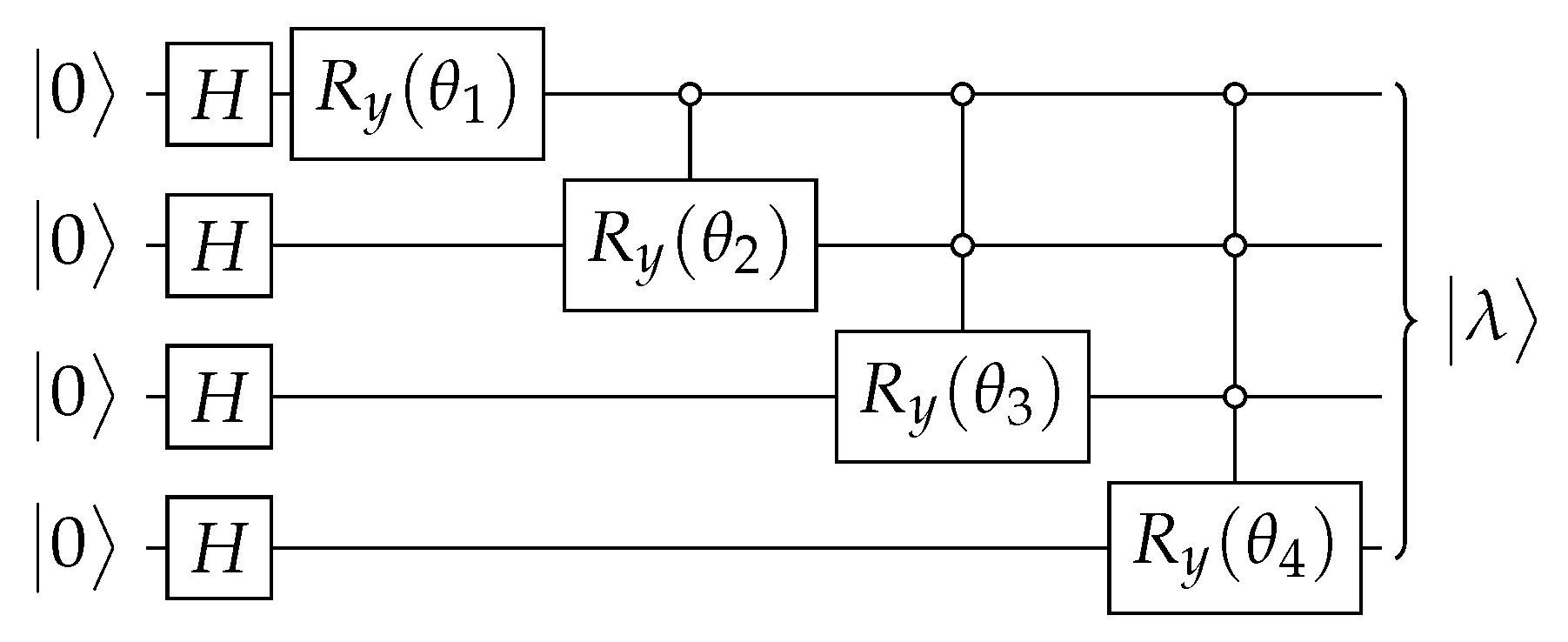
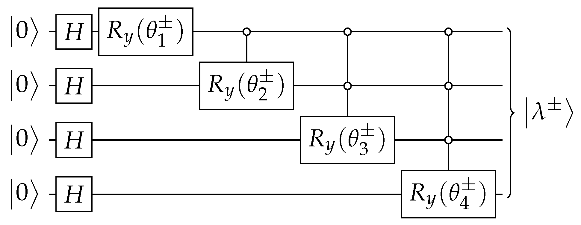
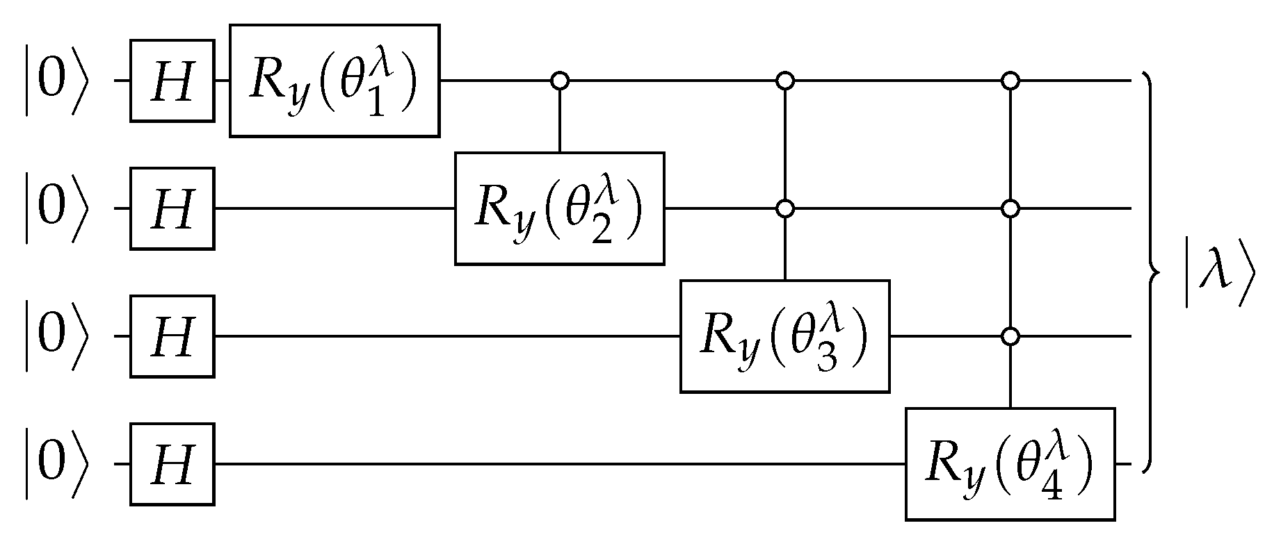
Appendix A. State Preparation
There is a well-known recipe for obtaining a circuit of an operator A that outputs a generic state of n qubits when the input is —that is,
If has real entries and has many repeated entries, as discussed below, the Ansatz of Figure A1 provides a simpler circuit that has basic gates assuming reasonable restrictions on . The goal is to obtain angles that are used as parameters of the multi-controlled gates, where
Define and
for , where is the computational basis. If , then we can find such that is the output of the circuit of Figure A1. To show this statement, we use the fact that the output of the circuit is
where
for and . Assuming that
we obtain the system of equations
for in terms of variables . The solution is obtained in a recursive way starting with equation and decreasing the index k of Equation (A7). We obtain
and then
To conclude, the circuit of Figure A1 outputs (A6) when angles are given by Equations (A5) and (A9).
Note that the entry of vector in (A6) plays a special role in the spatial search algorithm, because it is associated with the label of the marked vertex. If the label of the marked vertex is ℓ (assume that ℓ is even by now), we want to define . In this case, we have to change some empty controls of the -gates in the circuit of Figure A1 into solid controls. The recipe is as follows. Let us focus on the last gate of Figure A1, which has empty controls. We want this gate to be activated if the input is ℓ. We change from empty to solid all controls associated with bits 1 of ℓ. The same modifications must be applied to the preceding gates. On the other hand, if ℓ is odd, we have to do an extra change, not in terms of converting further empty into solid controls, but by changing into .
Appendix B. Eigenvectors of the Modified Hamiltonian
Suppose that the distinct eigenvalues of the adjacency matrix A are . Define as the orthogonal projector onto the eigenspace of A associated with eigenvalue for , so that
Let us assume that the asymptotic dynamics of the search algorithm depends only on two eigenvectors of H (1) associated with eigenvalues closest to , such as
where is the spectral gap. Refs. [25,28] shows that the computational complexity of the search algorithm with one marked vertex w is determined by two sums given by
and
and the asymptotic value of is obtained as
and
Asymptotically, the success probability is
and the optimal running time is
To calculate the success probability, we need two extra quantities that are (1) the overlap between and the marked vertex, which is
and (2) the overlap between and the initial state, which is
Now, we are ready to calculate an asymptotic expression for , that is, the -th entry of . These calculations go beyond the results of Refs. [25,28]. Let us assume that the initial condition is a linear combination of and in the asymptotic limit. Using the completeness relation, we obtain
where and are the unknowns. We obtain a second independent equation in these unknowns by sandwiching H as follows:
Using Equations (1) and (A10), we obtain
where
and assuming that is the uniform state. The solution of the system of Equations (A20) and (A21) is
The circuit of such that can be obtained using the techniques of Appendix A.
References
- Farhi, E.; Gutmann, S. Quantum computation and decision trees. Phys. Rev. A 1998, 58, 915–928. [Google Scholar] [CrossRef]
- Childs, A.M.; Goldstone, J. Spatial search by quantum walk. Phys. Rev. A 2004, 70, 022314. [Google Scholar] [CrossRef]
- Agliari, E.; Blumen, A.; Mülken, O. Quantum-walk approach to searching on fractal structures. Phys. Rev. A 2010, 82, 012305. [Google Scholar] [CrossRef]
- Philipp, P.; Tarrataca, L.; Boettcher, S. Continuous-time quantum search on balanced trees. Phys. Rev. A 2016, 93, 032305. [Google Scholar] [CrossRef]
- Osada, T.; Coutinho, B.; Omar, Y.; Sanaka, K.; Munro, W.J.; Nemoto, K. Continuous-time quantum-walk spatial search on the Bollobás scale-free network. Phys. Rev. A 2020, 101, 022310. [Google Scholar] [CrossRef]
- Malmi, J.; Rossi, M.A.C.; García-Pérez, G.; Maniscalco, S. Spatial search by continuous-time quantum walks on renormalized Internet networks. Phys. Rev. Res. 2022, 4, 043185. [Google Scholar] [CrossRef]
- Farhi, E.; Goldstone, J.; Gutmann, S. A Quantum Algorithm for the Hamiltonian NAND Tree. Theory Comput. 2008, 4, 169–190. [Google Scholar] [CrossRef]
- Childs, A.M. Universal Computation by Quantum Walk. Phys. Rev. Lett. 2009, 102, 180501. [Google Scholar] [CrossRef]
- Childs, A.M.; Gosset, D.; Webb, Z. Universal Computation by Multiparticle Quantum Walk. Science 2013, 339, 791–794. [Google Scholar] [CrossRef]
- Lahini, Y.; Steinbrecher, G.R.; Bookatz, A.D.; Englund, D. Quantum logic using correlated one-dimensional quantum walks. npj Quantum Inf. 2018, 4, 2. [Google Scholar] [CrossRef]
- Dadras, S.; Gresch, A.; Groiseau, C.; Wimberger, S.; Summy, G.S. Experimental realization of a momentum-space quantum walk. Phys. Rev. A 2019, 99, 043617. [Google Scholar] [CrossRef]
- Delvecchio, M.; Groiseau, C.; Petiziol, F.; Summy, G.S.; Wimberger, S. Quantum search with a continuous-time quantum walk in momentum space. J. Phys. B At. Mol. Opt. Phys. 2020, 53, 065301. [Google Scholar] [CrossRef]
- Wang, K.; Shi, Y.; Xiao, L.; Wang, J.; Joglekar, Y.N.; Xue, P. Experimental realization of continuous-time quantum walks on directed graphs and their application in PageRank. Optica 2020, 7, 1524–1530. [Google Scholar] [CrossRef]
- Benedetti, C.; Tamascelli, D.; Paris, M.G.; Crespi, A. Quantum Spatial Search in Two-Dimensional Waveguide Arrays. Phys. Rev. Appl. 2021, 16, 054036. [Google Scholar] [CrossRef]
- Qu, D.; Marsh, S.; Wang, K.; Xiao, L.; Wang, J.; Xue, P. Deterministic Search on Star Graphs via Quantum Walks. Phys. Rev. Lett. 2022, 128, 050501. [Google Scholar] [CrossRef]
- Qiang, X.; Loke, T.; Montanaro, A.; Aungskunsiri, K.; Zhou, X.; O’Brien, J.L.; Wang, J.B.; Matthews, J.C.F. Efficient quantum walk on a quantum processor. Nat. Commun. 2016, 7, 11511. [Google Scholar] [CrossRef] [PubMed]
- Loke, T.; Wang, J.B. Efficient quantum circuits for continuous-time quantum walks on composite graphs. J. Phys. A Math. Theor. 2017, 50, 055303. [Google Scholar] [CrossRef]
- Santos, J.; Chagas, B.; Chaves, R. Quantum Walks in a Superconducting Quantum Computer. In WQUANTUM; Sociedade Brasileira de Computação: Porto Alegre, Brasil, 2021; pp. 25–30. [Google Scholar] [CrossRef]
- Aharonov, Y.; Davidovich, L.; Zagury, N. Quantum random walks. Phys. Rev. A 1993, 48, 1687–1690. [Google Scholar] [CrossRef]
- Acasiete, F.; Agostini, F.P.; Moqadam, J.K.; Portugal, R. Implementation of quantum walks on IBM quantum computers. Quantum Inf. Process. 2020, 19, 426. [Google Scholar] [CrossRef]
- Nzongani, U.; Zylberman, J.; Doncecchi, C.E.; Pérez, A.; Debbasch, F.; Arnault, P. Quantum circuits for discrete-time quantum walks with position-dependent coin operator. Quantum Inf. Process. 2023, 22, 270. [Google Scholar] [CrossRef]
- Georgopoulos, K.; Emary, C.; Zuliani, P. Comparison of quantum-walk implementations on noisy intermediate-scale quantum computers. Phys. Rev. A 2021, 103, 022408. [Google Scholar] [CrossRef]
- Wing-Bocanegra, A.; Venegas-Andraca, S.E. Circuit implementation of discrete-time quantum walks via the shunt decomposition method. Quantum Inf. Process. 2023, 22, 146. [Google Scholar] [CrossRef]
- Razzoli, L.; Cenedese, G.; Bondani, M.; Benenti, G. Efficient Implementation of Discrete-Time Quantum Walks on Quantum Computers. Entropy 2024, 26. [Google Scholar] [CrossRef]
- Lugão, P.; Portugal, R.; Sabri, M.; Tanaka, H. Multimarked Spatial Search by Continuous-Time Quantum Walk. ACM Trans. Quantum Comput. 2024, 5. [Google Scholar] [CrossRef]
- Frigerio, M.; Benedetti, C.; Olivares, S.; Paris, M.G.A. Generalized quantum-classical correspondence for random walks on graphs. Phys. Rev. A 2021, 104, L030201. [Google Scholar] [CrossRef]
- Bezerra, G.A.; Lugão, P.H.G.; Portugal, R. Quantum-walk-based search algorithms with multiple marked vertices. Phys. Rev. A 2021, 103, 062202. [Google Scholar] [CrossRef]
- Silva, C.F.T.d.; Posner, D.; Portugal, R. Walking on vertices and edges by continuous-time quantum walk. Quantum Inf. Process. 2023, 22, 93. [Google Scholar] [CrossRef]
Disclaimer/Publisher’s Note: The statements, opinions and data contained in all publications are solely those of the individual author(s) and contributor(s) and not of MDPI and/or the editor(s). MDPI and/or the editor(s) disclaim responsibility for any injury to people or property resulting from any ideas, methods, instructions or products referred to in the content. |
© 2025 by the authors. Licensee MDPI, Basel, Switzerland. This article is an open access article distributed under the terms and conditions of the Creative Commons Attribution (CC BY) license (https://creativecommons.org/licenses/by/4.0/).