Sustainability of a Three-Species Predator–Prey Model in Tumor-Immune Dynamics with Periodic Treatment

Abstract

Using a tumor-immune growth model, we investigate how immunotherapy affects its dynamical characteristics. Specifically, we extend the prey–predator model of tumor cells and immune cells by including periodic immunotherapy, the nonlinear damping of cancer cells, and the dynamics of a healthy cell population, and investigate the effects of the model parameters. The ideal value of immunotherapy, which promotes the growth of immune (and healthy) cells while contributing to the elimination or control of the cancer cells, is determined by using Fisher information as a measure of variability throughout our study.

1. Introduction

The predator–prey model provides a valuable framework for understanding the population dynamics of different species in nature [1,2,3,4,5]. The simplest form of this model is represented by the two-species Lotka–Volterra equations:

$$\begin{array}{c}\hfill \begin{array}{c}\hfill {\displaystyle \frac{dx}{dt}}=ax-bxy,\\ \hfill {\displaystyle \frac{dy}{dt}}=-cy+exy,\end{array}\end{array}$$

(1)

which describe the interaction between the prey population x and the predator population y. Here, a, b, c, and e are positive parameters that represent the growth rate of prey (intrinsic rate of increase in the prey population), mortality of prey due to predation, the mortality rate of predators, and the growth of predators from the consumption of prey, respectively. This model was originally developed by Lotka (1925) [6] and Volterra (1926) [7] to describe the population dynamics of prey fish (x) and predator sharks (y). If competition between the two species is not excessively strong, the two populations can co-exist in a stable way and exhibit a limit cycle behavior [1,3,8,9,10,11,12,13].

This paper aims to extend the predator–prey model by incorporating an information-theoretic perspective. Specifically, we used Fisher information to analyze the sustainability of the model in Equation (1). Fisher information, a measure of system order and predictability, has been increasingly used in ecological and complex system analysis. Applying it to tumor-immune dynamics allows for a novel assessment of the sustainability and stability of the system. In our study, we reinterpret x and y as cancer and immune cells, respectively, and extend the model to include (i) the effect of immunotherapy modeled as an oscillatory forcing term, (ii) competition effects through logistic growth, and (iii) the dynamics of healthy cells. To better capture real-world tumor-immune interactions, we extend the model by incorporating an oscillatory immunotherapy term, competition effects, and the role of healthy cells, which play a critical role in tumor dynamics. A key focus of this study is immunotherapy, a promising therapeutic approach that improves the immune system’s ability to eliminate cancer cells through external stimulation [14,15,16,17,18,19]. In our previous work, we conducted a detailed investigation of the two-species model, where x and y in Equation (1) were analyzed in depth [20]. Although predator–prey models provide a useful mathematical framework for studying interactions between cancer and immune cells, they must be modified to incorporate immune suppression, activation thresholds, and external interventions. The analogy is useful but requires adjustments to fully capture the biological complexity of the tumor-immune dynamics.

The remainder of this paper is organized as follows. Section 2 introduces the three-species model, while Section 3 presents the extended version. Finally, the conclusions are drawn in Section 4. The appendices provide additional details, including Fisher information calculations for the logistic equation and the extended three-species model.

2. Three-Species Model

We extend the two-species model [20] to the three-species model by including the dynamics of the population of healthy cells and look into how periodic disturbance affects the evolution of the system to figure out how the oscillatory behavior of immunotherapy treatment survives for a long time and remains unchanged at certain parameter values. By including immunotherapy ($F{sin}^2\left(\omega t\right)$), we intend to show how the performance of the three-species model changes and to clarify how periodic therapy affects the behavior of the species from an information theory perspective.

Our model is given as follows:

$$\begin{array}{c}\hfill {\displaystyle \frac{dx}{dt}}=ax(1-N_{1}x)-bxy-dxz,\end{array}$$

(2a)

$$\begin{array}{c}\hfill {\displaystyle \frac{dy}{dt}}=-cy+{\displaystyle \frac{kyx}{g_2+x}}-fyx+F{sin}^2\left(\omega t\right),\end{array}$$

(2b)

$$\begin{array}{c}\hfill {\displaystyle \frac{dz}{dt}}=gz(1-N_{2}z)-hzx.\end{array}$$

(2c)

Here, x, y, and z represents cancer cell population, the populations of healthy cells and immune cells, respectively. Taking into account two alternative carrying capacities, $N_1$ (>0) and $N_2$ (>0), respectively, we consider the growth of healthy populations and cancer to be logistic. Cancer cell growth is represented by a (>0), immune cell growth by k (>0), and healthy cell growth by g (>0). c (>0) is the natural mortality rate of immune cells. The rate at which immune cells prey on cancer cells is b (>0), while the rate at which cancer cells prey on immune cells is f (>0). The rate at which cancer cells prey on healthy cells is d (>0), while the rate at which cancer cells prey on healthy cells is h (>0). The periodic treatment amplitude is F, and its angular frequency is $\omega$. We include the Michaelis–Menten form in the second term in Equation (2b) to model the saturated effects (with positive constants $g_2,\alpha >0$) of the immune reaction (the finite interaction between immune cells and cancer cells) (see [9,21]).

We rescale the model in (2) to minimize the number of parameters in the following dimensionless form:

$$\begin{array}{ccc}\hfill {\displaystyle \frac{du}{d\mathcal{T}}}& =& u(1-u)-uv-a_{13}ur,\hfill \\ \hfill {\displaystyle \frac{dv}{d\mathcal{T}}}& =& a_{21}[{\displaystyle \frac{uv}{g_2+\alpha u}}-v]-a_{22}uv+a_{23}{\sin }^2(\Omega \mathcal{T}),\hfill \\ \hfill {\displaystyle \frac{dr}{d\mathcal{T}}}& =& a_{31}r(1-r)-a_{32}ru.\hfill \end{array}$$

(3)

Here, similarly, u, v and r represent the population of cancer cells, immune cells, and healthy cells, respectively. Note that $a_{23}$ in Equation (3) corresponds to F in Equation (2). Equation (3) involves two competition modes. That is, in addition to the competition between cancer cells u and immune cells v in the predator–prey style, Equation (3) now has a new competition between healthy cells r and cancer cells u on the available resources. To understand the effect of periodic treatment $a_{23}{sin}^2(\Omega \mathcal{T})$, we perform a set of numerical simulations of the Equation (3) considering a set of parameters such as $a_{13}=1.2$, $a_{21}=1.291$, $g_2=0.3$, $\alpha =1$, $a_{22}=1.1$, $a_{31}=1.2$, $a_{32}=4.8$, and $\Omega =1$ together with the initial condition $u_0=v_0=r_0=1$ (which are similar to those used in [22]).

Local Stability Analysis and Equilibria

To gain a key insight into the dynamics of our model, we use the mean value of the periodic treatment and find the stationary points. $(0,\frac{a_{23}}{2a_{21}},0)$, $(0,\frac{a_{23}}{2a_{21}},1)$, $(u^{*},v^{*},r^{*})=(1-v^{*},v^{*},0)$, where $v^{*}$ is the solution to the following equation:

$$\begin{array}{c}\hfill \begin{array}{c}\hfill a_{21}\left[{\displaystyle \frac{v(1-v)}{g_2+\alpha (1-v)}}-v\right]-a_{22}v(1-v)+{\displaystyle \frac{a_{23}}{2}}=0.\end{array}\end{array}$$

The last effective equilibrium point is $(u^{**},v^{**},r^{**})=(\frac{a_{31}{v}^{**}+a_{31}(a_{13}-1)}{a_{32}{a}_{13}-a_{31}},v^{**}$, $\frac{a_{32}-a_{31}-a_{32}{v}^{**}}{a_{32}{a}_{13}-a_{31}})$, where $v^{**}$ is the solution to the following equation:

$$\begin{array}{c}\hfill \begin{array}{c}\hfill a_{21}\left[{\displaystyle \frac{v\left(\frac{a_{31}v+a_{31}(a_{13}-1)}{a_{32}{a}_{13}-a_{31}}\right)}{g_2+\alpha \left(\frac{a_{31}v+a_{31}(a_{13}-1)}{a_{32}{a}_{13}-a_{31}}\right)}}-v\right]-a_{22}v\left({\displaystyle \frac{a_{31}v+a_{31}(a_{13}-1)}{a_{32}{a}_{13}-a_{31}}}\right)+{\displaystyle \frac{a_{23}}{2}}=0.\end{array}\end{array}$$

For the stability analysis of the above stationary points, it is useful to fix the values of the parameters and examine the effect of treatment by varying their $a_{23}$. The point $(0,0.3873,1)$ has three negative eigenvalues (smaller than zero), while the first point $(0,0.3873,0)$ is a saddle point with one negative eigenvalue and two positive eigenvalues when $a_{23}=1$. This results in a stable solution where cancer cells are zero and only healthy and immune cells are present.

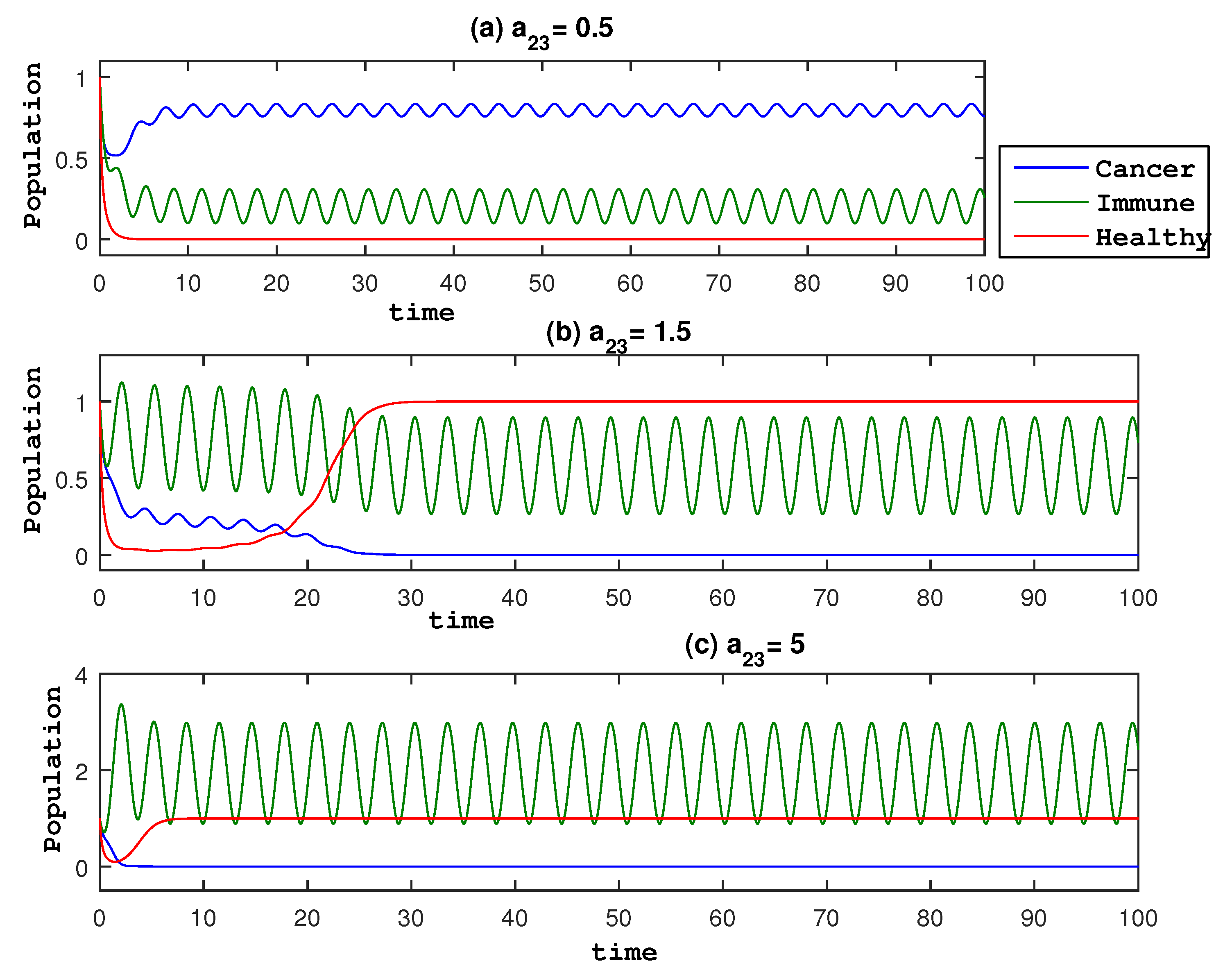
To understand the dynamics of the model in (3), we show time traces of u and v and phase portraits in Figure 1 by varying the amplitude of the periodic treatment $a_{23}$. Three rows in Figure 1 are for different values of $a_{23}$. When $a_{23}=5$, we observe that the time trace and phase portrait in the bottom panels show a small value of the cancer cell in the limit of a long time. In comparison, for a smaller value of $a_{23}$ shown in the top and middle panels, cancer cells take a finite value in the long time limit. These demonstrate the effect of periodic treatment on the elimination of the cancer population. Also, from Figure 1, we can observe that the higher the amplitude $a_{23}$, the better, as cancer cells begin to vanish and the immune system begins to increase. This suggests that it is advantageous to look at each species’ average at various $a_{23}$ values, as well as to determine the optimal value of $a_{23}$ in which the cancer cell population is eliminated. The right panels are a phase portrait for each $a_{23}$ after removing the initial transient.

To this end, in Figure 2, we present the mean values of $u,v,r$ for different values of $a_{23}$. In Figure 2, the eradication of the cancer population occurs at an amplitude $a_{23}=1.5$ that is smaller compared to the model of two species (without healthy cells) (amplitude $F=2.62$). This means that healthy cells help to eliminate cancer cells and thus the optimal value of the amplitude of the treatment is smaller in the three-species model. It is also interesting to see that in Figure 3, the healthy population is almost in a steady state with the value 1 in the long time limit. On the other hand, the immune population increases as $a_{23}$ increases. These results are the consequence of a stable effective equilibrium point $(0,\frac{a_{23}}{2a_{21}},1)$.

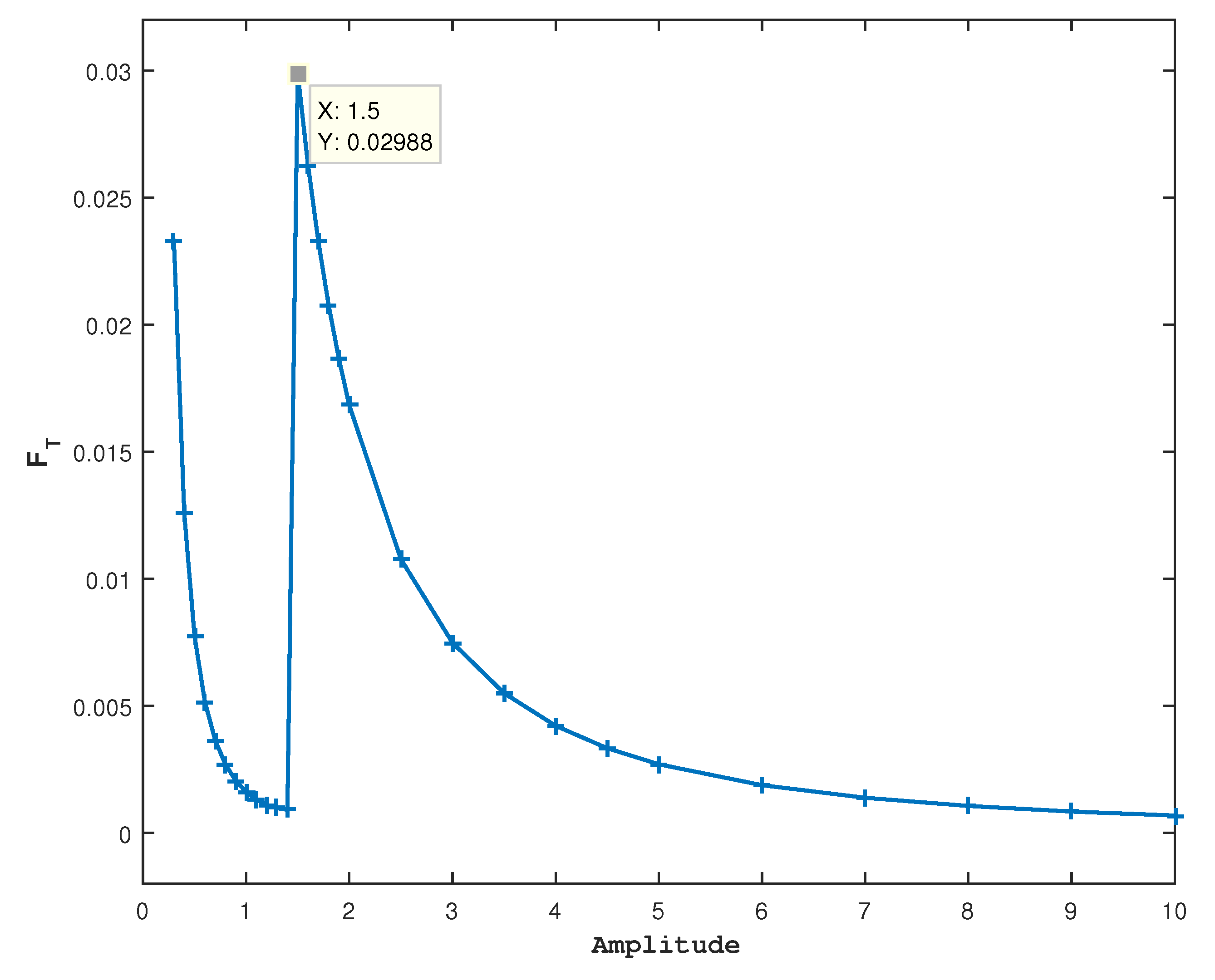
For our main purpose of understanding the variability/sustainability of the tumor-immune system [23], we now compute the Fisher information $F_T$ (see Appendix A.2 and Appendix A.4) at different values of amplitude $a_{23}$, and Figure 4 presents the results.

In Figure 4, a prominent peak in $F_T$ is observed in $a_{23}=1.5$ which is the optimal value of the amplitude to eradicate tumor cells. This state is unsustainable and less variable because of the loss of one species. The large value of $F_T$ means a low disorder and is related to a narrow PDF. Further increases in $a_{23}$ cause a decrease in $F_T$, similarly to what was observed in the two-species model.

3. Extended Three-Species Model

We further extend the model in Equation (3) including fluctuation (or variability) in the cancer growth rate modeled by $ϵsin\left({\Omega }_1\mathcal{T}\right)$ as

$$\begin{array}{c}\hfill \begin{array}{c}\hfill {\displaystyle \frac{du}{d\mathcal{T}}}=(1+ϵsin\left({\Omega }_1\mathcal{T}\right))u(1-u)-uv-a_{13}ur,\\ \hfill {\displaystyle \frac{dv}{d\mathcal{T}}}=a_{21}[{\displaystyle \frac{uv}{g_2+\alpha u}}-v]-a_{22}uv+a_{23}{sin}^2(\Omega \mathcal{T}),\\ \hfill {\displaystyle \frac{dr}{d\mathcal{T}}}=a_{31}r(1-r)-a_{32}ur.\end{array}\end{array}$$

(4)

Here, again, u, v and r represent the population of cancer cells, immune cells, and healthy cells, respectively. The only difference between the two models is in the equations. Equations (3) and (4) show the fluctuation in the growth of cancer cells.

To show the effect of fluctuation on the cancer growth rate, we fixed all parameter values to $a_{13}=1.2$, $a_{21}=1.291$, $g_2=0.3$, $\alpha =1$, $a_{22}=1.1$, $a_{31}=1.2$, $a_{32}=4.8$, in addition to $\Omega ={\Omega }_1=1$ and different values of $a_{23}$. In Figure 5, we present the results for different $ϵ$. Compared to Figure 2, we observe a similar behavior in Figure 5 without a significant effect of $ϵ$. In all panels, the cancer population starts to vanish roughly around $a_{23}=1.5$. To examine its fluctuation at this value, we present $F_T$ in Figure 6 using $ϵ=0.1$.

In Figure 6, we again observe a distinct maximum of $F_T$ at $a_{23}=1.5$, quite similar to Figure 4. This leads us to the conclusion that there is no significant change induced by $ϵ$.

3.1. Effects of $ϵ$

To study the effect of $ϵ$ systematically, it is useful to fix $a_{23}$, $\Omega$, ${\Omega }_1$ and vary $ϵ$.

Thus, we fix $a_{23}=1.5$, $\Omega ={\Omega }_1=1$ and all other parameter values mentioned in the above text and vary $ϵ$, and show the results in Figure 7. In all cases, we see that the three species approach the same final states. We confirm that $ϵ$ has no effect on long-term evolution by showing the plot of the average values of $u,v,r$ in model (4) for different values of $ϵ$ in Figure 8.

Using Fisher information, we compute $F_T$ for different $ϵ$ and fixed ${\Omega }_1$ to be ${\Omega }_1=1$ and the amplitude to be $a_{23}=1.5$ to determine the behavior of the model (4) in Figure 7 and Figure 8. The system in a steady-state solution does not lose or acquire Fisher information, as we can see by the fact that the $F_T$ values do not vary over time. Using $a_{23}=4$, we obtain a similar result.

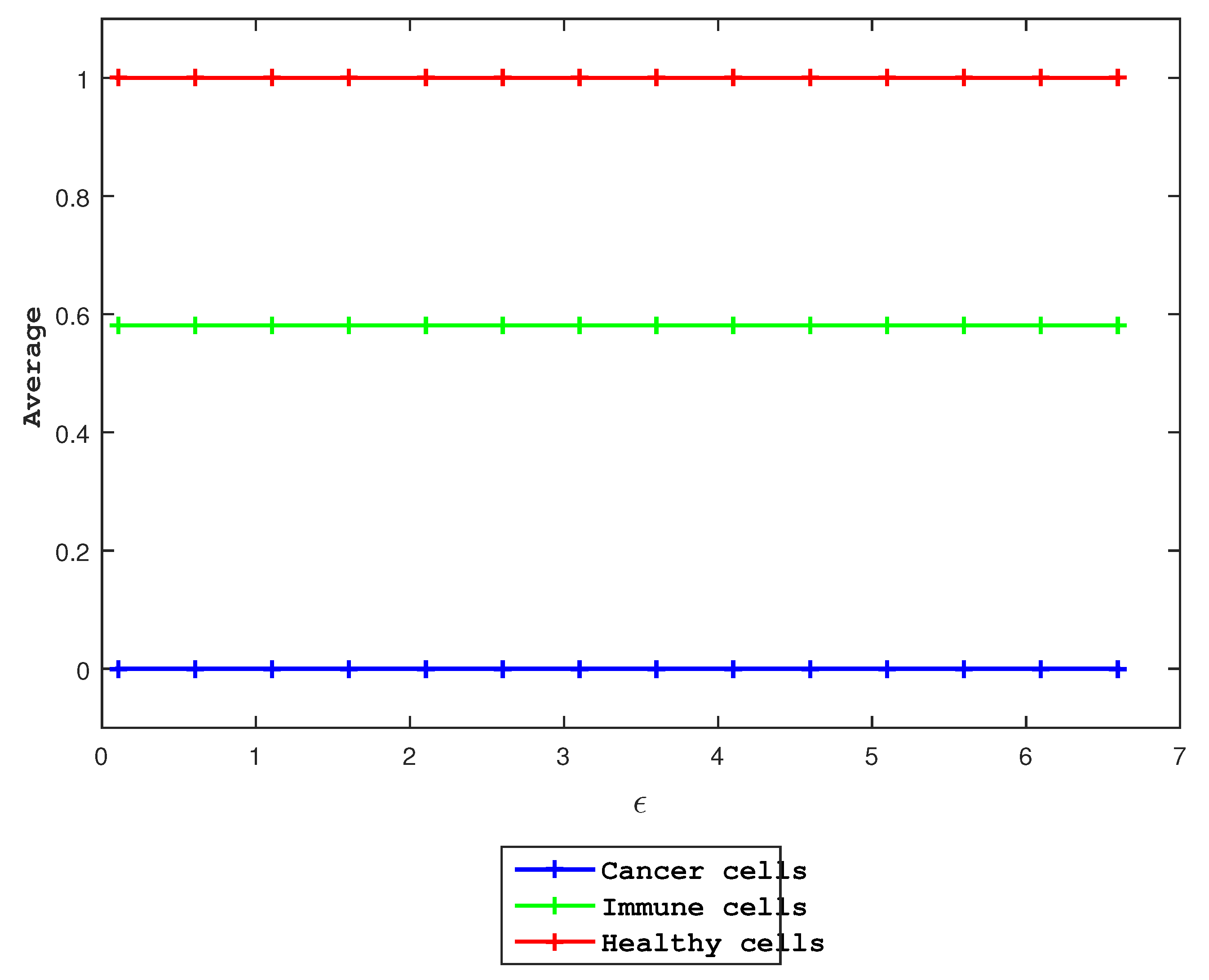
3.2. Effects of ${\Omega }_1$

Finally, we examine the effect of ${\Omega }_1$ in Equation (4). Specifically, we use the initial condition $u_0=v_0=r_0=1$ and the same other parameter values as mentioned above and vary ${\Omega }_1$. Clearly, the average values for the three species do not change when ${\Omega }_1$ increases.

4. Discussion

In this study, we investigated the impact of immunotherapy on the dynamical properties of a tumor-immune healthy-cell model by extending the classical predator–prey framework to a three-species system. The addition of periodic immunotherapy, non-linear damping of cancer cells, and the dynamics of healthy cells allowed us to explore a more comprehensive representation of tumor-immune interactions.

One of the key findings is that the introduction of immunotherapy leads to significant changes in the dynamics of the system. Using Fisher information as a measure of variability, we identified an optimal immunotherapy value, $a_{23}=1.5$, which effectively reduces the tumor population while promoting the growth of healthy and immune cells. Compared to the two-species model, the three-species model demonstrates a more pronounced ability to suppress cancer growth, highlighting the importance of incorporating healthy cell dynamics into tumor-immune models.

Furthermore, our study revealed that varying the prey killing rate (b, cancer death rate) results in a monotonic decrease in the equilibrium point. At a specific value of b, Fisher information reaches a maximum, corresponding to a state where the probability density functions (PDF) of tumor and immune cells become narrow and do not overlap, indicating a minimal interaction between species. This suggests that at this parameter value, the system may be in an undesirable state due to reduced variability and interaction among species.

Furthermore, when the amplitude of immunotherapy ($a_{23}$) was varied, we observed that higher values led to greater tumor suppression but also resulted in reduced variability in the dynamics of the system. This suggests a trade-off between effective tumor suppression and maintaining system dynamism, which could have implications for treatment strategies.

In general, our results emphasize the importance of optimizing immunotherapy parameters to achieve the best therapeutic outcomes. The incorporation of healthy cell dynamics into the model significantly alters the behavior of the system and leads to a lower optimal immunotherapy value compared to the two-species model. These findings provide insight into how tumor-immune health interactions respond to external treatments and contribute to a broader understanding of cancer therapy dynamics.

5. Conclusions

This study examined the influence of immunotherapy on the dynamical properties of a tumor-immune healthy cell system using an extended predator–prey model. By incorporating periodic immunotherapy and the dynamics of healthy cells, we identified key parameter values that optimize treatment effectiveness.

The optimal value of immunotherapy ($a_{23}=1.5$) promotes the growth of healthy and immune cells while reducing the tumor population, demonstrating the significant impact of including healthy cell dynamics in tumor modeling. Additionally, Fisher information analysis highlighted the importance of variability in system behavior, with specific parameter values leading to reduced interaction between species.

These findings provide valuable information on the complex interplay between tumor cells, immune responses, and treatment strategies. Our study could contribute to refining immunotherapy protocols and optimizing dosage strategies for cancer treatment, one of the world’s leading causes of death.

While our study primarily focuses on analyzing the effects of immunotherapy using Fisher information, we acknowledge that averaging state variables may obscure complex dynamical behaviors. A more detailed bifurcation analysis could provide deeper insights into stability transitions, periodic oscillations, or chaotic dynamics in the system. Due to the scope of this work, a full bifurcation analysis was not included. However, future studies could incorporate bifurcation diagrams to complement our findings and further explore the nonlinear behavior of tumor-immune interactions under varying immunotherapy conditions.

References

- Shastri, Y.; Diwekar, U. Sustainable ecosystem management using optimal control theory: Part 2 (stochastic systems). J. Theor. Biol. 2006, 2006, 522–532. [Google Scholar] [CrossRef]
- Cabezas, H.; Fath, B.D. Towards a theory of sustainable systems. Fluid Phase Equilibria 2002, 2002, 3–14. [Google Scholar] [CrossRef]
- Fath, B.D.; Cabezas, H.; Pawlowski, C.W. Regime changes in ecological systems: An information theory approach. J. Theor. Biol. 2003, 2003, 517–530. [Google Scholar] [CrossRef]
- Abrams, P.A. Why don’t predators have positive effects on prey populations? Evol. Ecol. 1992, 1992, 449–457. [Google Scholar] [CrossRef]
- Kumar, S.M.; Sharma, A.; Sánchez-Ruiz, L.M. Dynamical Complexity of Modified Leslie—Gower Predator–Prey Model Incorporating Double Allee Effect and Fear Effect. Symmetry 2024, 2024, 1552. [Google Scholar]
- Lotka, A.J. Elements of Physical Biology; Hassell Street Press: Victoria, Australia, 1925. [Google Scholar]
- Volterra, V. Fluctuations in the abundance of a species considered mathematically. Nature 1926, 118, 558–560. [Google Scholar] [CrossRef]
- Mayer, A.L.; Pawlowski, C.W.; Cabezas, H. Fisher information and dynamic regime changes in ecological systems. Ecol. Model. 2006, 2006, 72–82. [Google Scholar] [CrossRef]
- Rico-Ramirez, V.; Reyes-Mendoza, M.A.; Quintana-Hernez, P.A.; Ortiz-Cruz, J.A.; Hernez-Castro, S.; Diwekar, U.M. Fisher information on the performance of dynamic systems. Ind. Eng. Chem. Res. 2010, 2010, 1812–1821. [Google Scholar] [CrossRef]
- Érika, D.; Otero-Espinar, M.V. Predator–prey models: A review of some recent advances. Mathematics 2021, 2021, 1783. [Google Scholar]
- Murray, J.D. Mathematical Biology: I. An Introduction; Springer: New York, NY, USA, 2002. [Google Scholar]
- Selin, N.E.; Giang, A.; Clark, W.C. Progress in modeling dynamic systems for sustainable development. Proc. Natl. Acad. Sci. USA 2023, 120, e2216656120. [Google Scholar] [CrossRef]
- Banerjee, S.; Sarkar, R.R. Delay-induced model for tumor-immune interaction and control of malignant tumor growth. Biosystems 2008, 2008, 268–288. [Google Scholar] [CrossRef]
- Joseph, M.K.; Ouifki, R.; Eladdadi, A.; de Pillis, L. Mathematical model of tumor–immune surveillance. J. Theor. Biol. 2016, 2016, 312–330. [Google Scholar]
- d’Onofrio, A. A general framework for modeling tumor-immune system competition and immunotherapy: Mathematical analysis and biomedical inferences. Phys. Nonlinear Phenom. 2005, 2005, 220–235. [Google Scholar] [CrossRef]
- Windarto, W.; Eridani, E. On modification and application of Lotka-Volterra competition model. Aip Conf. Proc. 2020, 2268, 050007. [Google Scholar]
- Wu, Y.; Tur, A.; Wang, H. Sustainable Optimal Control for Switched Pollution-Control Problem with Random Duration. Entropy 2023, 25, 1426. [Google Scholar] [CrossRef]
- Amany, N.; Albalawi, W.; Jazmati, M.S.; Elrashidi, A.; Ali, H.M.; Moaaz, O. Functional Differential Equations with an Advanced Neutral Term: New Monotonic Properties of Recursive Nature to Optimize Oscillation Criteria. Axioms 2024, 2024, 847. [Google Scholar]
- Kareva, I.; Luddy, K.A.; O’Farrelly, C.; Gatenby, R.A.; Brown, J.S. Predator-Prey in Tumor-Immune Interactions: A Wrong Model or Just an Incomplete One? Front. Immunol. 2021, 12, 668221. [Google Scholar] [CrossRef] [PubMed] [PubMed Central]
- Al-Saffar, A.; Kim, E. Fisher Information Approach in Modified Predator—Prey Model. Axioms 2025, 14, 144. [Google Scholar] [CrossRef]
- Kirschner, D.; Panetta, J.C. Modeling immunotherapy of the tumor-immune interaction. J. Math. Biol. 1998, 1998, 235–252. [Google Scholar] [CrossRef]
- López, Á.G.; Sabuco, J.; Seoane, J.M.; Duarte, J.; Januário, C.; Sanjuán, M.A.F. Avoiding healthy cells extinction in a cancer model. J. Theor. Biol. 2014, 2014, 74–81. [Google Scholar] [CrossRef]
- Sahbani, M.; Das, S.; Green, J.R. Classical Fisher information for differentiable dynamical systems. Chaos: An Interdisciplinary. J. Nonlinear Sci. 2023, 33, 103139. [Google Scholar]
- Al-Saffar, A.; Kim, E. Sustainable theory of a logistic model-Fisher Information approach. Math. Biosci. 2017, 2017, 81–91. [Google Scholar] [CrossRef] [PubMed]
- Al-Saffar, A.; Kim, E. Fisher information approach to understand the Gompertz model. Math. Appl. Sci. Eng. 2022, 2022, 269–279. [Google Scholar] [CrossRef]
Figure 1.
Phase portrait and time evolution of Equations (
3) for various
,
. Green indicates immune cells, red indicates healthy cells, and a blue line indicates cancer.
Figure 2.
Average values as a function of periodic amplitude, with all parameter values fixed, , and changed.
Figure 3.
Time evolution of x using different values, .
Figure 4.
For
and fixed other parameter values,
is shown against the amplitude. In
Figure 2 and
Figure 3, a peak is observed at
, which is also the value at which the cancer cells start to disappear.
Figure 5.
For , populations’ average values are shown against the amplitude , with being different and the other parameter values fixed. A red line indicates healthy cells, a green line indicates immune cells, and a blue line indicates cancer cells.
Figure 6.
The amplitude
against
for
, and
: At
, a peak is shown, which is also the value at which the cancer cells begin to disappear in
Figure 7.
To show the dynamics of the model with fixed parameter values as , , and , we utilize different values of . Red indicates healthy cells, green indicates immune cells, and blue indicates cancer cells.
Figure 8.
As a function of , we show the average of each species in various colors, while the other parameters remain unchanged. The average values show no changes, indicating that our model is independent of .