
Three-Phase Confusion Learning


Abstract
1. Introduction
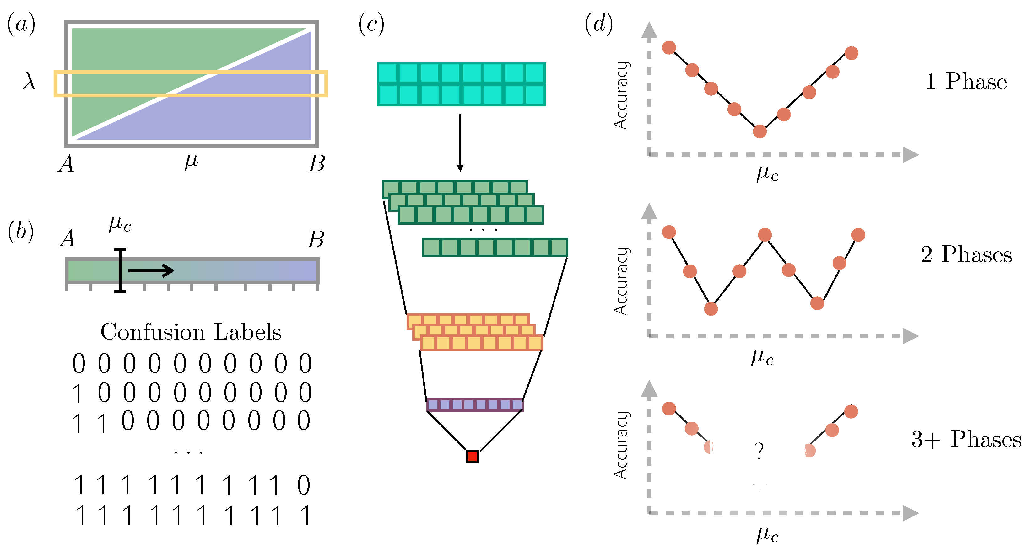
2. Confusion Learning
2.1. Two-Phase Learning
2.2. Three-Phase Learning
3. Results
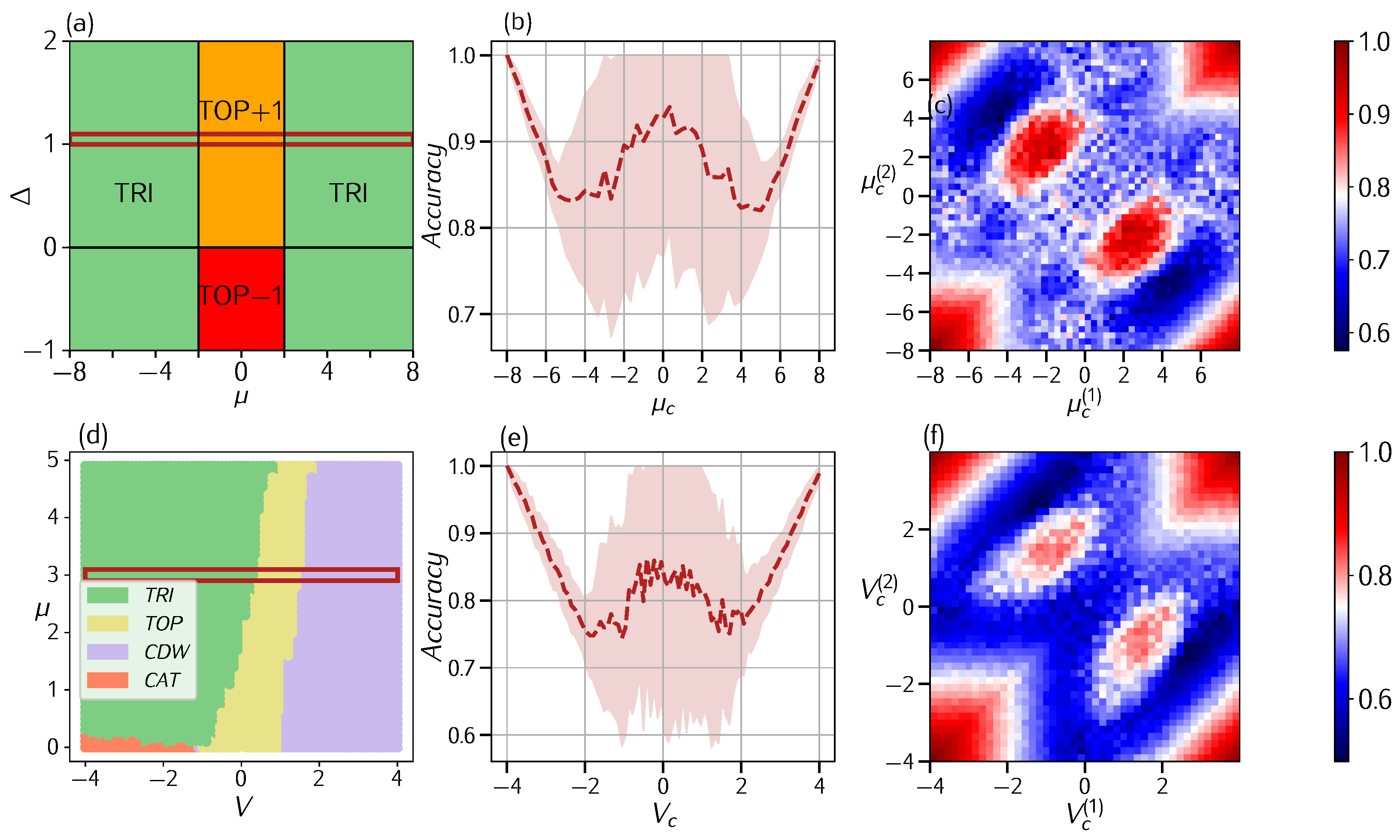
3.1. Kitaev Chain
3.1.1. Free Model
3.1.2. Interacting Model
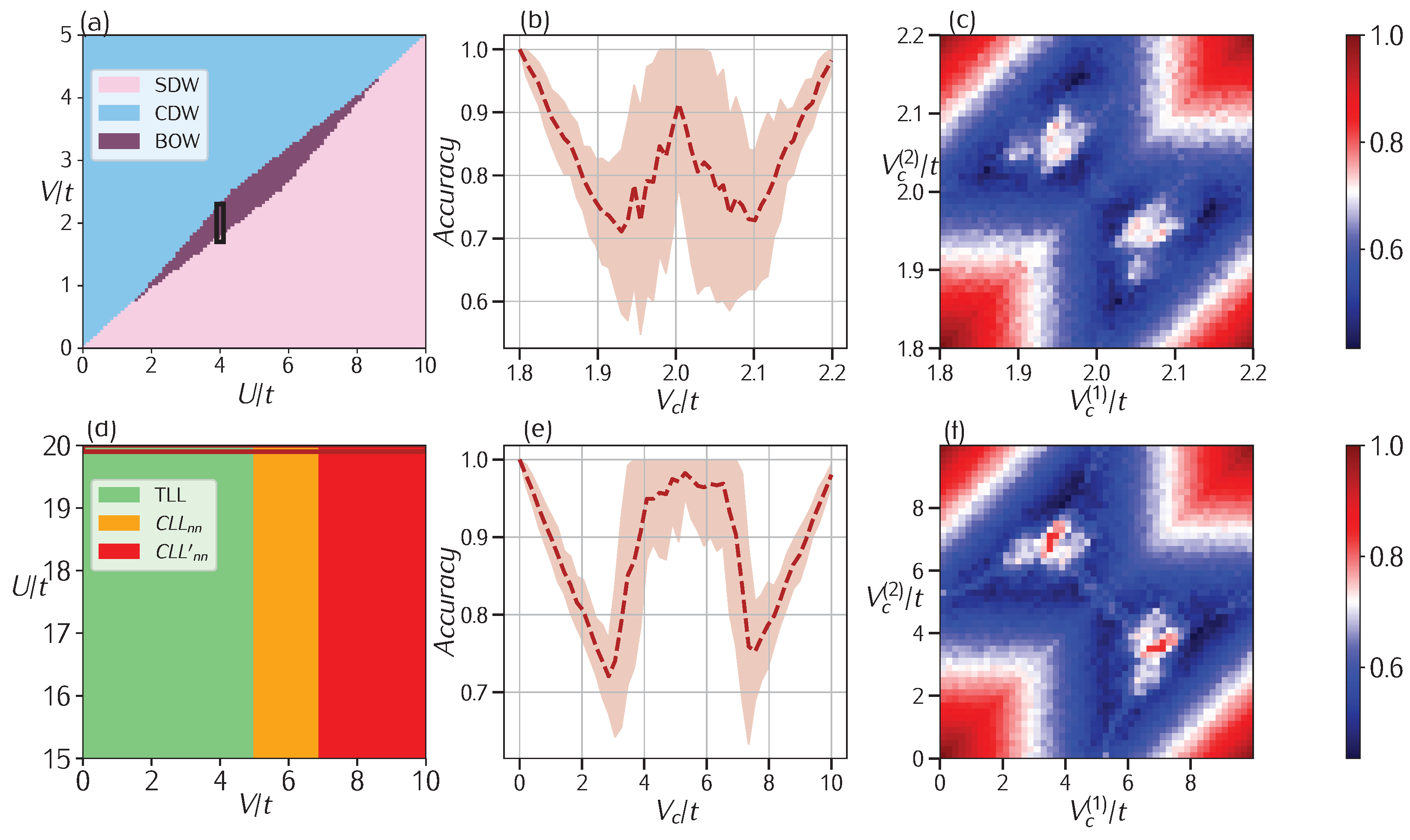
3.2. Extended Hubbard
3.2.1. Model
3.2.2. Model
4. Conclusions
Author Contributions
Funding
Data Availability Statement
Conflicts of Interest
Abbreviations
| PBC | Periodic Boundary Condition |
| DMRG | Density Matrix Renormalization Group |
| CNN | Convolutional Neural Network |
Appendix A. Data and CNN Details
Appendix A.1. Kitaev Chain Data
Appendix A.2. Hubbard Model
Appendix A.3. CNN
References
- Sutherland, B. Beautiful Models; World Scientific: Singapore, 2004. [Google Scholar] [CrossRef]
- Sandvik, A.W.; Avella, A.; Mancini, F. Computational Studies of Quantum Spin Systems. AIP Conf. Proc. 2010, 1297, 135–338. [Google Scholar] [CrossRef]
- Schollwöck, U. The density-matrix renormalization group in the age of matrix product states. Ann. Phys. 2011, 326, 96–192. [Google Scholar] [CrossRef]
- Becca, F.; Sorella, S. Quantum Monte Carlo Approaches for Correlated Systems; Cambridge University Press: Cambridge, UK, 2017. [Google Scholar]
- Tibaldi, S.; Magnifico, G.; Vodola, D.; Ercolessi, E. Unsupervised and supervised learning of interacting topological phases from single-particle correlation functions. SciPost Phys. 2023, 14, 005. [Google Scholar] [CrossRef]
- Caleca, F.; Tibaldi, S.; Botzung, T.; Pupillo, G.; Ercolessi, E. Unsupervised learning of unknown phases in the 1D quantum extended Fermi-Hubbard model with soft-shoulder potential. In preparation.
- Rodriguez-Nieva, J.F.; Scheurer, M.S. Identifying topological order through unsupervised machine learning. Nat. Phys. 2019, 15, 790–795. [Google Scholar] [CrossRef]
- Long, Y.; Ren, J.; Chen, H. Unsupervised Manifold Clustering of Topological Phononics. Phys. Rev. Lett. 2020, 124, 185501. [Google Scholar] [CrossRef]
- Scheurer, M.S.; Slager, R.J. Unsupervised Machine Learning and Band Topology. Phys. Rev. Lett. 2020, 124, 226401. [Google Scholar] [CrossRef]
- Che, Y.; Gneiting, C.; Liu, T.; Nori, F. Topological quantum phase transitions retrieved through unsupervised machine learning. Phys. Rev. B 2020, 102, 134213. [Google Scholar] [CrossRef]
- Lustig, E.; Yair, O.; Talmon, R.; Segev, M. Identifying Topological Phase Transitions in Experiments Using Manifold Learning. Phys. Rev. Lett. 2020, 125, 127401. [Google Scholar] [CrossRef]
- Lidiak, A.; Gong, Z. Unsupervised Machine Learning of Quantum Phase Transitions Using Diffusion Maps. Phys. Rev. Lett. 2020, 125, 225701. [Google Scholar] [CrossRef]
- Long, Y.; Zhang, B. Unsupervised Data-Driven Classification of Topological Gapped Systems with Symmetries. Phys. Rev. Lett. 2023, 130, 036601. [Google Scholar] [CrossRef]
- Rem, B.S.; Käming, N.; Tarnowski, M.; Asteria, L.; Fläschner, N.; Becker, C.; Sengstock, K.; Weitenberg, C. Identifying quantum phase transitions using artificial neural networks on experimental data. Nat. Phys. 2019, 15, 917–920. [Google Scholar] [CrossRef]
- van Nieuwenburg, E.P.L.; Liu, Y.H.; Huber, S.D. Learning phase transitions by confusion. Nat. Phys. 2017, 13, 435–439. [Google Scholar] [CrossRef]
- Richter-Laskowska, M.; Kurpas, M.; Maśka, M.M. Learning by confusion approach to identification of discontinuous phase transitions. Phys. Rev. E 2023, 108, 024113. [Google Scholar] [CrossRef] [PubMed]
- Corte, I.; Acevedo, S.; Arlego, M.; Lamas, C. Exploring neural network training strategies to determine phase transitions in frustrated magnetic models. Comput. Mater. Sci. 2021, 198, 110702. [Google Scholar] [CrossRef]
- Wang, R.; Ma, Y.G.; Wada, R.; Chen, L.W.; He, W.B.; Liu, H.L.; Sun, K.J. Nuclear liquid-gas phase transition with machine learning. Phys. Rev. Res. 2020, 2, 043202. [Google Scholar] [CrossRef]
- Gavreev, M.A.; Mastiukova, A.S.; Kiktenko, E.O.; Fedorov, A.K. Learning entanglement breakdown as a phase transition by confusion. New J. Phys. 2022, 24, 073045. [Google Scholar] [CrossRef]
- Lee, S.S.; Kim, B.J. Confusion scheme in machine learning detects double phase transitions and quasi-long-range order. Phys. Rev. E 2019, 99, 043308. [Google Scholar] [CrossRef]
- Arnold, J.; Schäfer, F.; Edelman, A.; Bruder, C. Mapping Out Phase Diagrams with Generative Classifiers. Phys. Rev. Lett. 2024, 132, 207301. [Google Scholar] [CrossRef]
- Arnold, J.; Schäfer, F.; Lörch, N. Fast Detection of Phase Transitions with Multi-Task Learning-by-Confusion. arXiv 2023, arXiv:2311.09128. [Google Scholar]
- Dawid, A.; Arnold, J.; Requena, B.; Gresch, A.; Płodzień, M.; Donatella, K.; Nicoli, K.A.; Stornati, P.; Koch, R.; Büttner, M.; et al. Modern applications of machine learning in quantum sciences. arXiv 2022, arXiv:2204.04198. [Google Scholar] [CrossRef]
- Richter-Laskowska, M.; Kurpas, M.; Maśka, M. A learning by confusion approach to characterize phase transitions. arXiv 2022, arXiv:2206.15114. [Google Scholar]
- Sun, Z. Pattern Recognition in Convolutional Neural Network (CNN). In Proceedings of the Application of Intelligent Systems in Multi-modal Information Analytics, Online, 23 April 2022; Sugumaran, V., Sreedevi, A.G., Xu, Z., Eds.; Springer: Cham, Switzerland, 2022; pp. 295–302. [Google Scholar]
- Zhang, W.; Zeng, Z. Research Progress of Convolutional Neural Network and its Application in Object Detection. arXiv 2020, arXiv:2007.13284. [Google Scholar] [CrossRef]
- Krizhevsky, A.; Sutskever, I.; Hinton, G.E. ImageNet Classification with Deep Convolutional Neural Networks. In Advances in Neural Information Processing Systems; Pereira, F., Burges, C., Bottou, L., Weinberger, K., Eds.; Curran Associates, Inc.: New York, NY, USA, 2012; Volume 25. [Google Scholar]
- Zhang, Q.; Zhang, M.; Chen, T.; Sun, Z.; Ma, Y.; Yu, B. Recent Advances in Convolutional Neural Network Acceleration. arXiv 2018, arXiv:1807.08596. [Google Scholar] [CrossRef]
- Kitaev, A.Y. Unpaired Majorana fermions in quantum wires. Physics-Uspekhi 2001, 44, 131–136. [Google Scholar] [CrossRef]
- Schnyder, A.P.; Ryu, S.; Furusaki, A.; Ludwig, A.W.W. Classification of topological insulators and superconductors in three spatial dimensions. Phys. Rev. B 2008, 78, 195125. [Google Scholar] [CrossRef]
- Chiu, C.K.; Teo, J.C.Y.; Schnyder, A.P.; Ryu, S. Classification of topological quantum matter with symmetries. Rev. Mod. Phys. 2016, 88, 035005. [Google Scholar] [CrossRef]
- Slager, R.J.; Mesaros, A.; Juričić, V.; Zaanen, J. The space group classification of topological band-insulators. Nat. Phys. 2013, 9, 98–102. [Google Scholar] [CrossRef]
- Ryu, S.; Schnyder, A.P.; Furusaki, A.; Ludwig, A.W.W. Topological insulators and superconductors: Tenfold way and dimensional hierarchy. New J. Phys. 2010, 12, 065010. [Google Scholar] [CrossRef]
- Stoudenmire, E.M.; Alicea, J.; Starykh, O.A.; Fisher, M.P. Interaction effects in topological superconducting wires supporting Majorana fermions. Phys. Rev. B 2011, 84, 014503. [Google Scholar] [CrossRef]
- Hassler, F.; Schuricht, D. Strongly interacting Majorana modes in an array of Josephson Junctions. New J. Phys. 2012, 14, 125018. [Google Scholar] [CrossRef]
- Thomale, R.; Rachel, S.; Schmitteckert, P. Tunneling spectra simulation of interacting Majorana wires. Phys. Rev. B 2013, 88, 161103. [Google Scholar] [CrossRef]
- Katsura, H.; Schuricht, D.; Takahashi, M. Exact ground states and topological order in interacting Kitaev/Majorana chains. Phys. Rev. B 2015, 92, 115137. [Google Scholar] [CrossRef]
- Miao, J.J. Exact Solution for the Interacting Kitaev Chain at the Symmetric Point. Phys. Rev. Lett. 2017, 118. [Google Scholar] [CrossRef] [PubMed]
- Fromholz, P.; Magnifico, G.; Vitale, V.; Mendes-Santos, T.; Dalmonte, M. Entanglement topological invariants for one-dimensional topological superconductors. Phys. Rev. B 2020, 101, 085136. [Google Scholar] [CrossRef]
- Schollwöck, U. The density-matrix renormalization group. Rev. Mod. Phys. 2005, 77, 259–315. [Google Scholar] [CrossRef]
- Fishman, M.; White, S.R.; Stoudenmire, E.M. The ITensor Software Library for Tensor Network Calculations. arXiv 2020, arXiv:2007.14822. [Google Scholar] [CrossRef]
- Arovas, D.P.; Berg, E.; Kivelson, S.A.; Raghu, S. The Hubbard Model. Annu. Rev. Condens. Matter Phys. 2022, 13, 239–274. [Google Scholar] [CrossRef]
- Tasaki, H. The Hubbard Model: Introduction and Selected Rigorous Results. arXiv 1997, arXiv:cond-mat/9512169. [Google Scholar] [CrossRef]
- Desaules, J.Y.; Hudomal, A.; Turner, C.J.; Papić, Z. Proposal for Realizing Quantum Scars in the Tilted 1D Fermi-Hubbard Model. Phys. Rev. Lett. 2021, 126, 210601. [Google Scholar] [CrossRef]
- Hensgens, T.; Fujita, T.; Janssen, L.; Li, X.; Van Diepen, C.J.; Reichl, C.; Wegscheider, W.; Das Sarma, S.; Vandersypen, L.M. Quantum simulation of a Fermi–Hubbard model using a semiconductor quantum dot array. Nature 2017, 548, 70–73. [Google Scholar] [CrossRef]
- Tarruell, L.; Sanchez-Palencia, L. Quantum simulation of the Hubbard model with ultracold fermions in optical lattices. arXiv 2019, arXiv:1809.00571. [Google Scholar] [CrossRef]
- Robaszkiewicz, S.; Bułka, B.R. Superconductivity in the Hubbard model with pair hopping. Phys. Rev. B 1999, 59, 6430–6437. [Google Scholar] [CrossRef]
- Dong, X.; Re, L.D.; Toschi, A.; Gull, E. Mechanism of superconductivity in the Hubbard model at intermediate interaction strength. Proc. Natl. Acad. Sci. USA 2022, 119, e2205048119. [Google Scholar] [CrossRef] [PubMed]
- Nakamura, M. Tricritical behavior in the extended Hubbard chains. Phys. Rev. B 2000, 61, 16377–16392. [Google Scholar] [CrossRef]
- Ejima, S.; Nishimoto, S. Phase Diagram of the One-Dimensional Half-Filled Extended Hubbard Model. Phys. Rev. Lett. 2007, 99, 216403. [Google Scholar] [CrossRef]
- Hirsch, J.E. Charge-Density-Wave to Spin-Density-Wave Transition in the Extended Hubbard Model. Phys. Rev. Lett. 1984, 53, 2327–2330. [Google Scholar] [CrossRef]
- Cannon, J.; Fradkin, E. Phase diagram of the extended Hubbard model in one spatial dimension. Phys. Rev. B 1990, 41, 9435–9443. [Google Scholar] [CrossRef]
- Mello, P.A.; Stone, A.D. Maximum-entropy model for quantum-mechanical interference effects in metallic conductors. Phys. Rev. B 1991, 44, 3559–3576. [Google Scholar] [CrossRef]
- van Dongen, P.G.J. Extended Hubbard model at strong coupling. Phys. Rev. B 1994, 49, 7904–7915. [Google Scholar] [CrossRef]
- Voit, J. One-dimensional Fermi liquids. Rep. Prog. Phys. 1995, 58, 977. [Google Scholar] [CrossRef]
- Tsuchiizu, M.; Furusaki, A. Phase Diagram of the One-Dimensional Extended Hubbard Model at Half Filling. Phys. Rev. Lett. 2002, 88, 056402. [Google Scholar] [CrossRef] [PubMed]
- Tam, K.M.; Tsai, S.W.; Campbell, D.K. Functional Renormalization Group Analysis of the Half-Filled One-Dimensional Extended Hubbard Model. Phys. Rev. Lett. 2006, 96, 036408. [Google Scholar] [CrossRef] [PubMed]
- Jeckelmann, E. Ground-State Phase Diagram of a Half-Filled One-Dimensional Extended Hubbard Model. Phys. Rev. Lett. 2002, 89, 236401. [Google Scholar] [CrossRef]
- Sengupta, P.; Sandvik, A.W.; Campbell, D.K. Bond-order-wave phase and quantum phase transitions in the one-dimensional extended Hubbard model. Phys. Rev. B 2002, 65, 155113. [Google Scholar] [CrossRef]
- Sandvik, A.W.; Balents, L.; Campbell, D.K. Ground State Phases of the Half-Filled One-Dimensional Extended Hubbard Model. Phys. Rev. Lett. 2004, 92, 236401. [Google Scholar] [CrossRef]
- Zhang, Y.Z. Dimerization in a Half-Filled One-Dimensional Extended Hubbard Model. Phys. Rev. Lett. 2004, 92, 246404. [Google Scholar] [CrossRef]
- Glocke, S.; Klümper, A.; Sirker, J. Half-filled one-dimensional extended Hubbard model: Phase diagram and thermodynamics. Phys. Rev. B 2007, 76, 155121. [Google Scholar] [CrossRef]
- Botzung, T. Study of Strongly Correlated One-Dimensional Systems with Long-Range Interactions. Ph.D. Thesis, Université de Strasbourg, Strasbourg, France, 2019. [Google Scholar]
- Caleca, F. Machine Learning Approach to the Extended Hubbard Model. Master’s Thesis, University of Bologna, Bologna, Italy, 2021. [Google Scholar]
- Mattioli, M.; Dalmonte, M.; Lechner, W.; Pupillo, G. Cluster Luttinger Liquids of Rydberg-Dressed Atoms in Optical Lattices. Phys. Rev. Lett. 2013, 111, 165302. [Google Scholar] [CrossRef]
- Dalmonte, M.; Lechner, W.; Cai, Z.; Mattioli, M.; Läuchli, A.M.; Pupillo, G. Cluster Luttinger liquids and emergent supersymmetric conformal critical points in the one-dimensional soft-shoulder Hubbard model. Phys. Rev. B 2015, 92, 045106. [Google Scholar] [CrossRef]
Disclaimer/Publisher’s Note: The statements, opinions and data contained in all publications are solely those of the individual author(s) and contributor(s) and not of MDPI and/or the editor(s). MDPI and/or the editor(s) disclaim responsibility for any injury to people or property resulting from any ideas, methods, instructions or products referred to in the content. |
© 2025 by the authors. Licensee MDPI, Basel, Switzerland. This article is an open access article distributed under the terms and conditions of the Creative Commons Attribution (CC BY) license (https://creativecommons.org/licenses/by/4.0/).
Share and Cite
Caleca, F.; Tibaldi, S.; Ercolessi, E. Three-Phase Confusion Learning. Entropy 2025, 27, 199. https://doi.org/10.3390/e27020199
Caleca F, Tibaldi S, Ercolessi E. Three-Phase Confusion Learning. Entropy. 2025; 27(2):199. https://doi.org/10.3390/e27020199
Chicago/Turabian StyleCaleca, Filippo, Simone Tibaldi, and Elisa Ercolessi. 2025. "Three-Phase Confusion Learning" Entropy 27, no. 2: 199. https://doi.org/10.3390/e27020199
APA StyleCaleca, F., Tibaldi, S., & Ercolessi, E. (2025). Three-Phase Confusion Learning. Entropy, 27(2), 199. https://doi.org/10.3390/e27020199