1. Introduction
The rapid advancement of quantum information has brought considerable attention to quantum entanglement [
1], which serves as the cornerstone technology in this field. Many theoretical foundations of quantum information technology, including quantum key distribution [
2], quantum teleportation [
3], quantum simulation [
4], and quantum true randomness [
5], are highly dependent on quantum entanglement. Additionally, quantum entanglement is key to comprehending many peculiar properties of quantum mechanics, such as quantum non-locality and quantum many-body systems. Given the crucial role of entanglement, it is important to explore entanglement theory and experimental methods for generating entangled states.
So far, enormous progress has been made in the generation of entanglement. For example, 219 beryllium ions [
6], 14-photon entanglement [
7], 500-cold-atom entanglement [
8], and 51-qubit superconducting entanglement [
9] have been generated. With the continuous improvement in the fundamental technology of quantum control, it is expected that larger quantum systems will soon become entangled. However, a common concern in experiments is ensuring that the underlying entanglement is indeed produced, especially for larger systems. This results in the quantum states produced by the experiment being unknown to us and requiring further verification or quantification. Confirming the presence or quantifying the degree of entanglement presents challenges because they cannot be directly observed by any physical device. Various approaches can be considered to address this problem [
10,
11,
12,
13,
14,
15,
16,
17,
18,
19,
20,
21,
22,
23,
24,
25]. However, some methods [
11,
12,
13,
14,
15,
16,
17] can only detect entanglement without quantification, while others [
18,
19,
20,
21,
22,
23,
24,
25], although capable of entanglement quantification, face limitations due to the high computational complexity. Quantum state tomography (QST) [
26,
27,
28,
29] is a standard method to reconstruct a quantum state by observing its density matrix. Then, based on the density matrix, the existence (with the entanglement criterion [
16]) or the quantification of the entanglement (with the entanglement measures [
18,
19,
20,
21,
22,
23,
24,
25]) can be calculated for the states generated in the experiments. However, such a procedure requires a large number of measurements that scale exponentially with the dimension of the quantum state. Although researchers have proposed compressed sensing methods [
28,
30] to improve the efficiency of QST by reducing measurement resources, the measurement settings for QST still require exponential resources.
In view of this, one may imagine a new scheme with desirable properties. First, a crucial requirement is that the scheme under consideration must be easy to implement and most importantly allow for fewer and easier-to-implement measurements. In addition, the scheme should be robust to noise. Moreover, most experiments today aim to generate an entanglement between more than two particles. Therefore, the scheme has to be capable of multipartite scenarios. Classical machine learning methods have been proven to be a good scheme for detecting and quantifying entanglements. The idea is to train the neural network with the outcome statistics data produced by measuring sample quantum states as features and the entanglement criterion or measures as sample labels. Ma [
31] and Gao [
32] used neural networks to optimize the coefficients of the CHSH inequality [
15] theoretically and experimentally so that more entanglement states violated the optimized CHSH inequality; however, this method cannot quantify the entanglement; that is, it only answers yes or no. Lin [
33,
34] successfully employed neural networks to utilize collective measurement probabilities of quantum states as feature inputs, achieving high-precision quantification of coherent information [
35] and relative entropy of entanglement [
36] in qudit systems. In addition, they applied variational quantum algorithms [
37] to seek optimal measurement strategies. However, when Lin [
33] attempted to quantify the GME of multipartite systems, the number of measurements they used grew exponentially. Furthermore, due to the complexity of GME computation, this method does not apply to noisy quantum states and is difficult to extend to multipartite systems. Moller [
38] quantified the GME of multipartite pure state systems using variational quantum algorithms. By successfully implementing this method on the IBM Quantum systems, they demonstrated its effectiveness in producing GHZ states using three, four, and five qubits. However, challenges remain when dealing with noisy quantum states. Researchers [
39,
40,
41] also quantified different entanglement measures, but their scalability to multipartite and applicability to noisy quantum states are weak.
This paper is based on squashed entanglement to establish a connection between local measurements and entanglement utilizing neural networks. The study accurately quantifies unknown multipartite entanglement states, demonstrating their effectiveness in both pure and noisy quantum states. This method offers remarkable applicability and efficiency by requiring a linear number of measurements, presenting an innovative approach to precisely quantifying unknown multipartite entanglement states. The structure of this paper is as follows: In
Section 2, we describe the selection of entanglement measures and measurement settings. The quantification of the entanglement of pure and mixed states is presented in
Section 3 and
Section 4, respectively. Finally,
Section 6 contains conclusions and future work.
3. Quantifying Multipartite
Entanglement Pure State Without Noise
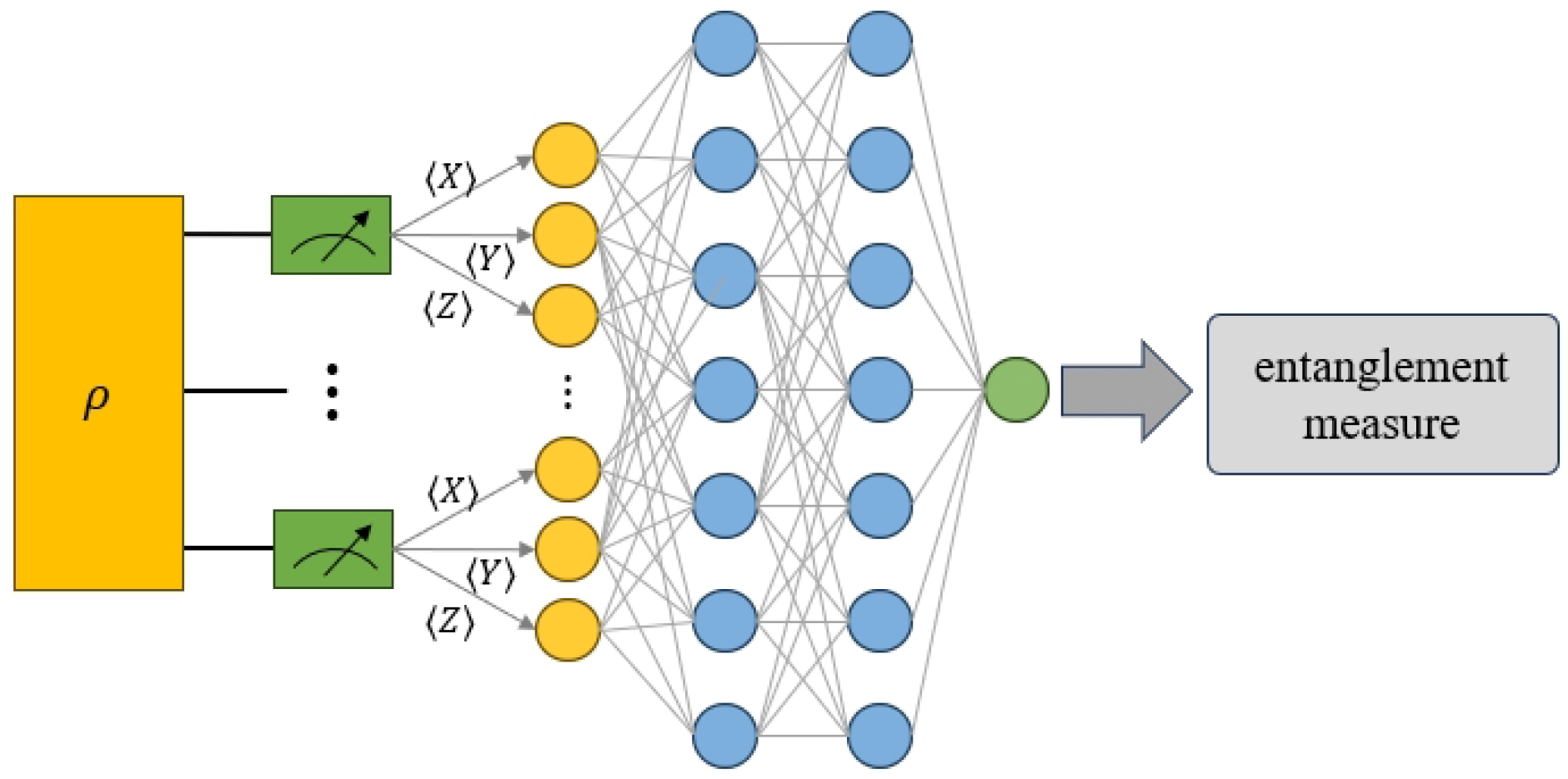
In the preceding description, the features and labels of the neural network have been introduced. At this stage, numerical simulation experiments will be conducted in pure states to verify whether the measurement settings in Equation (
11) can be used to predict the SE of the unknown multipartite quantum state. The workflow is illustrated in
Figure 1. We will employ random quantum states for training the neural network. The true SE values serve as labels, computed with Equation (
9), and the local measurement results, specified in Equation (
11), provide the features of these training states. Then, we will continuously optimize the parameters of the neural network to train it to predict the SE for unknown entanglement states.
We first generate a series of random state
which has the following form:
where the real and imaginary parts of the elements
are generated by a uniform distribution in the interval −1 to 1. The formula for calculating the SE of the pure state is Equation (
9). Since the SE of most of these states is very close to 1, it shows the entanglement of the randomly generated states is not uniformly distributed in the interval 0 to 1. To ensure that the trained neural network is able to predict all entanglements in 0 to 1, we then generate some random separable state:
and introduce a parameter
to make our random quantum state
look like the following form:
is the random quantum state we used for training the neural networks. For preparing the training samples, when we generate a random quantum state, we measure it and calculate its true entanglement with the SE formula in Equation (
9). We set the SE
with a step size of 0.1, and for each step, we choose 1000 random quantum states with this entanglement, resulting in a total of 10,000 training data.
This section focuses mainly on the performance of the neural network on multipartite systems without noise. We then describe the configuration parameters of the neural network selected in this work. The neural network is a network structure consisting of an input layer, an output layer, and several hidden layers, each containing multiple neurons. In this paper, a fully connected neural network is chosen, consisting of six hidden layers with 100, 200, 400, 500, 200, and 100 neurons, respectively. The input layer has
neurons, and the output layer has one neuron. The non-linear activation function,
, which can be defined as
is used between each layer. The loss function we chose is the Mean Square Error (MSE), which can be defined as follows:
where
is the exact value,
is the prediction value, and
N is the size of the dataset. The optimizer we chose is Adam [
48]. The learning rate was set to
.
Since the discovery of entanglement, researchers have explored various entanglement states, among which GHZ states and W states hold prominent positions in quantum mechanics [
49]. These states exhibit non-classical correlation properties in multipartite quantum systems, having significance in fields like quantum communication and quantum teleportation [
50,
51,
52,
53]. Due to the pivotal roles of the GHZ states and the W states in quantum information processing, we consider generalized versions of GHZ states and W states as the target states for testing. The test states we choose are in the following form:
and
where
and
, with a step size of 0.005.
The performance of the trained neural network in predicting entanglement for five-qubit and ten-qubit systems is shown in
Figure 2. It can be seen from the figure that the method proposed in this paper almost perfectly fits the true entanglement measures for both five-qubit and ten-qubit systems, demonstrating its efficiency and accuracy. For the five-qubit system, the error ranges for fitting
and
are as follows: the maximum errors are
and
, the minimum errors are
and
, and the MSE are
and
, respectively. Additionally, for the ten-qubit system, the maximum error for fitting
is
, the minimum error is
, and the MSE is
; the maximum error for fitting
is
, the minimum error is
, and the MSE is
. It can be seen from these data that the model exhibits excellent performance in fitting the test states.
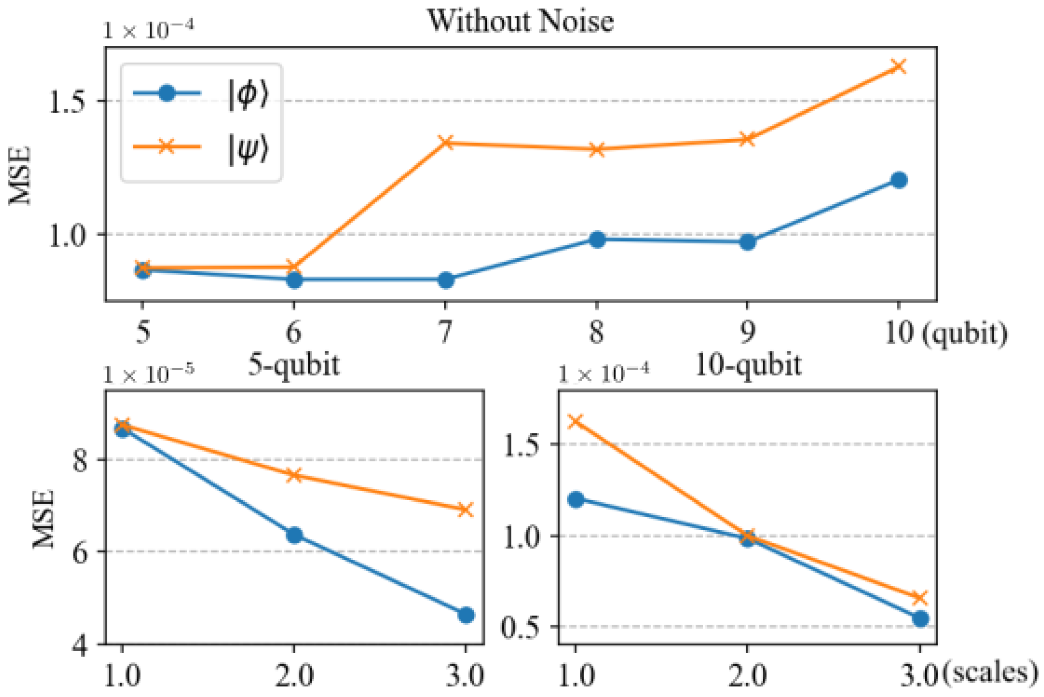
To further illustrate the effectiveness of the trained neural network, we also show the performance of the trained neural network in predicting entanglement for the test states shown in Equations (
18) and (
19) for the six-qubit to nine-qubit scenario. The results are shown in the upper figure of
Figure 3. Similarly to the experiment for the five-qubit and ten-qubit scenario,
p takes 0.05 as the step; thus, for each qubit number scenario, there are 200 data. We calculate the MSE for these test states and show them in
Figure 3. It can be seen that the MSEs for these states are around
; thus, the trained network fits these scenarios well. In addition, we note that with the increase in qubits from five to ten, the MSE shows a slight upward trend. This is because as the number of qubits increases, the dimension of the quantum state space grows exponentially, whereas the measurement method chosen in this paper only grows linearly. This mismatch in growth rates results in the loss of some information. However, it may be possible to improve this mismatch by increasing the number of neurons and the complexity of the model parameters. This is because larger models have more parameters, allowing them to more flexibly learn the complex features and patterns of the input data, thereby improving the model’s fitting ability. In addition, larger models typically better capture the non-linear relationships between data and have stronger generalization capabilities, performing better when faced with unseen data. In order to show whether prediction accuracy could be improved by increasing the size of the neural network model, we have introduced another two larger neural networks to predict the SE of the test states, and the results are shown in the lower figures of
Figure 3. It can be seen that by increasing the size of the neural network model, the prediction accuracy continuously improves. Although increasing the size of the neural network model helps improve the accuracy of the prediction, the number of training parameters required is approximately 0.42 million, 1.68 million, and 3.78 million, respectively, which leads to increased training costs. However, the method proposed in this paper achieves high-precision predictions with fewer training parameters and within an acceptable error range. If further improvement in accuracy is required, increasing the size of the neural network model moderately may be considered. This approach can balance the relationship between accuracy and training costs while meeting the requirements of practical applications.
We also present boxplots of the errors that visualize the error distribution, including its central tendency and dispersion. Boxplots provide an intuitive way to observe data distribution, helping to understand the accuracy of model predictions. In the previous description, MSE was used as an error metric. However, MSE is not intuitive because it squares the errors, resulting in units that are inconsistent with the original data units. Therefore,
Figure 4 shows the mean absolute error (MAE), representing the absolute difference between predicted and true values, to more intuitively present the distribution of errors. From
Figure 4, we can compare the errors between different test states and numbers of qubits. It can be observed that although prediction accuracy may decrease with an increase in the number of qubits, most prediction errors are within the range of 0 to 0.02. This indicates that even when dealing with larger-scale quantum systems, neural networks can still predict entanglement measures relatively accurately.
The results above demonstrate the excellent performance of the method proposed in this paper for quantifying pure unknown multipartite entanglement states. With the continuous advancement of quantum technologies, larger-scale entanglement systems will be created in the future [
54], and the method proposed in this paper provides a promising approach for studying these entanglement systems. This research opens up new possibilities for exploring more complex quantum entanglement phenomena, with the potential to drive advancements in the field of quantum information processing and play important roles in quantum computing, quantum communication, and other fields.
To further assess the performance of our model, we examine its ability to predict quantum random states. Specifically, we randomly generate 200 quantum states with qubit numbers ranging from
to
, in the form of Equation (
13), which represents a kind of Haar random state. For each case, we calculate the MSE between the actual and predicted values for the 200 states. The results, as shown in
Table 1, indicate that the MSE is around
or
, demonstrating the effectiveness of our trained model in predicting random states. This outcome is not unexpected, as the states used for network training follow the form of Equation (
13), which involves interference with separable states based on the structure outlined in Equation (
14).
4. Quantifying Multipartite
Entanglement Pure State in Noise Case
In the description of the idealized scenarios, we considered a closed system. However, real-world quantum systems are rarely completely closed. Quantum systems typically undergo inevitable interactions with their surroundings, and these interactions manifest themselves as various forms of noise within the quantum system. This noise can arise from environmental factors, impurities, and imperfections in the quantum devices themselves [
55]. Noise is also a major challenge in quantum technology. It can lead to information loss, causing severe impacts on applications that require high reliability, such as quantum computing and quantum communication. Noise may also induce irreversible losses in quantum states and interfere with qubits, limiting the performance of quantum systems. In the process of preparation of quantum states [
56], noise often has an impact, leading to the manifestation of quantum states as mixed states. In practical applications of current quantum devices, focusing solely on entanglement quantification of pure states is no longer sufficient. Therefore, to more comprehensively adapt to the characteristics of modern quantum technology, we will further investigate the influence of the noise. We concentrate on depolarizing noise and random channel noise, two prevalent types of quantum noise. Depolarizing noise generally results from flaws in quantum gate operations, causing the qubit to become a random mixture of all possible states, effectively “depolarizing” it into a mixed state.
where
represents the density matrix and
s represents the probability.
Then, we consider a more general case, random channel noise, often described as bit-flip or phase-flip noise. Random channel noise can originate from multiple sources, including physical channel imperfections in qubit interactions or from external factors like electromagnetic interference. In random channel noise, each party may randomly generate bit flipand phase flip. Bit-flip noise introduces probabilistic changes in the bit values, potentially causing alterations in qubits that were originally in an entanglement state, thus disrupting their entanglement. On the other hand, phase-flip noise introduces randomness in the phase of quantum states, which may disturb specific phase relationships and consequently affect the maintenance and transmission of entangled states. Formally, they can be defined as [
55]
for each party, where
, and
represents the probability of the corresponding noise events. We use Equation (
23) to apply channel noise to each qubit. After transmission in this quantum noise channel, the quantum state becomes the following:
In the case of random channel noise, this section will also employ the form after the action of Equation (
24) as the decomposition of mixed states.
Figure 5 shows the results of data fitting for noise entanglement systems, with a specific focus on a five-qubit entanglement system, where SE is used to measure the entanglement of the noisy state. However, as mentioned in
Section 2, quantifying entanglement in mixed states involves examining all potential decompositions of the state to determine the minimum value of Equation (
5), which is impractical. With the entropy inequality, Equation (
10) provides a lower bound for the C-SE across all possible state decompositions. We use the noise decomposition given in the paper as an approximation of the entanglement (Equation (
24) for states under channel noise, and computational bases for
I for depolarizing noise); the actual value may be higher than our approximation. However, because Equation (
10) establishes a lower bound, the value derived from the given decomposition can also be lower than the true entanglement value. In our numerical experiments, the probability of depolarizing noise is set to 0.1. This moderate noise is often used to simulate a typical experimental environment where quantum gates and qubits are imperfect but not completely noisy. The noise level is realistic for near-term quantum devices in the Noisy Intermediate-Scale Quantum (NISQ) era, where noise is present but the quantum algorithms can still be executed with some error correction or mitigation techniques. Conversely, for channel noise, due to the accumulation of noise in each qubit system, the overall noise becomes significant, which increases the likelihood of a large deviation from the original state. Therefore, to ensure the efficiency of prediction, the probability of channel noise could not be set too high. Here, we choose the small value 0.02 as an example. For depolarizing noise, the error ranges for fitting test states
and
are as follows: the maximum errors are
and
, the minimum errors are
and
, and the MSE are
and
. Furthermore, for channel noise, the maximum error for fitting
is
, the minimum error is
, and the MSE is
; the maximum error for fitting
is
, the minimum error is
, and the MSE is
. From this, it can be seen that the predictive performance is also excellent. Furthermore, from
Figure 5, it can also be observed that negative values appear in the SE calculation process for the subset of
in the five-qubit system, leading to the appearance of negative values in the predicted results. This is because, in the study of mixed states, the calculated SE is not an exact value, but an estimate. When negative values occur, the method proposed in this paper may not accurately identify entanglement, which is a limitation of our approach. However, it still provides an approximation of the entanglement for the quantum states with noise.
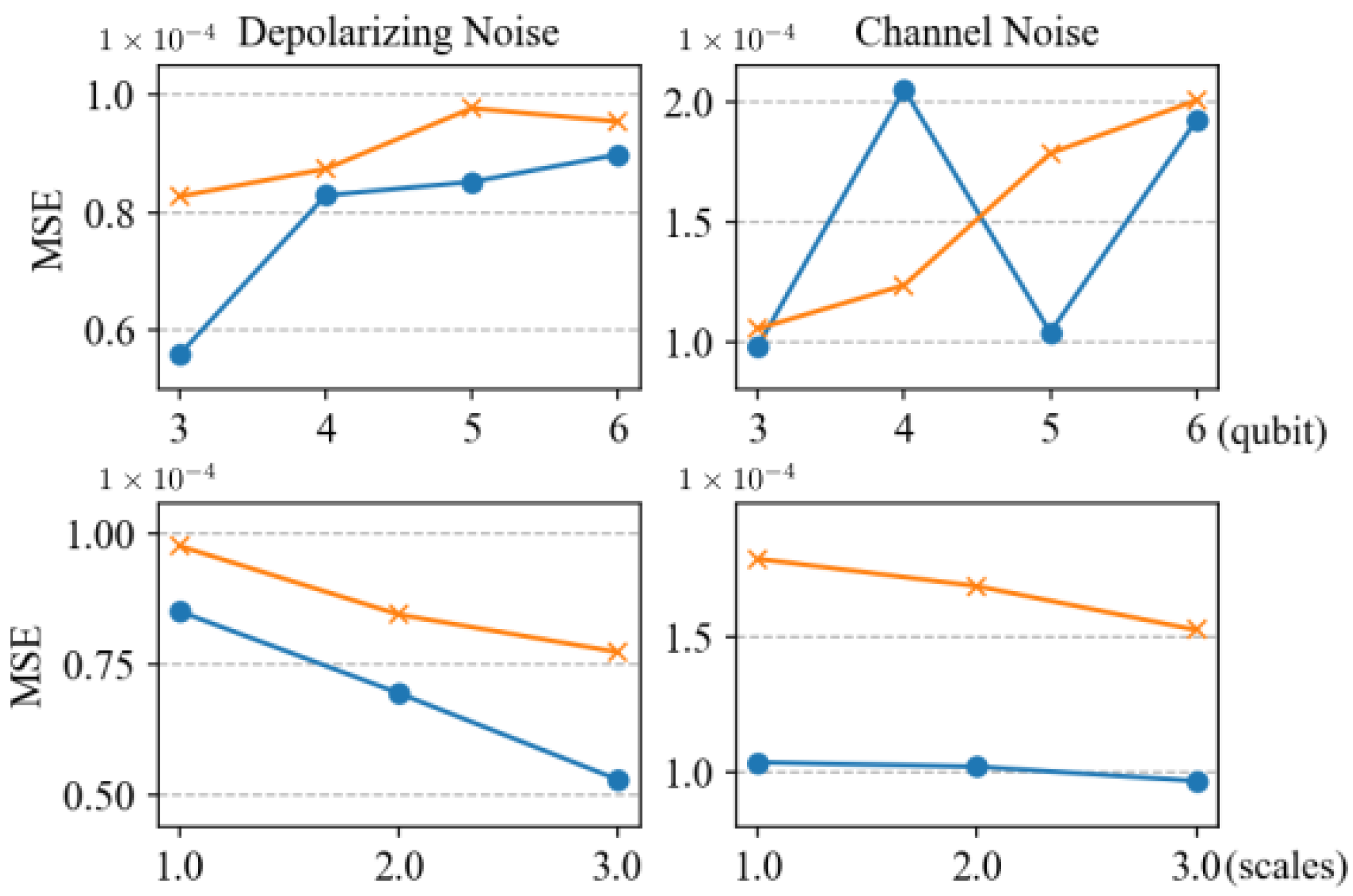
Figure 6 illustrates the MSE for predictions from three-qubit systems to six-qubit systems, and the corresponding boxplots of prediction errors are presented in
Figure 7. The phenomena observed in these figures and the reasons behind them are similar to those in the case without noise. In the presence of noise, the method proposed in this paper demonstrates excellent robustness. Compared to predicting pure states, the accuracy of predicting mixed states is slightly reduced. This phenomenon arises because mixed states possess more complex entanglement structures relative to pure states, and computing SE in the case of mixed states is more complicated. When calculating SE for mixed states, the last term in Equation (
10) needs to be considered, which involves information about the entire system, increasing the difficulty of prediction. The method proposed in this paper relies mainly on local measurement results as feature inputs, without collective measurements, leading to some information loss. However, despite these challenges, our method still demonstrates satisfactory performance in handling mixed-state tasks. Furthermore, it can be observed that, compared to channel noise, the prediction performance is better for depolarizing noise. This is due to noise build-up in each qubit system, resulting in a low probability of state preservation. The computation of the entanglement entropy (SE) for mixed states requires traversing the entire decomposition space, which amplifies the error between estimated and true values under noise, thereby reducing predictive efficacy.
Furthermore, it can be observed from the top-right subplot in
Figure 6 that under channel noise, the prediction error for the four-qubit entanglement system is relatively large. This is because for the four-qubit test state
, the expectation under the Pauli-X basis measurement is 0, while it is not 0 under other conditions. This results in multiple test states having the same features, increasing the difficulty of neural network prediction. Additionally, performing predictions under channel noise is inherently challenging because the introduction of noise makes the system’s behavior more complex and uncertain.
The observations above indicate that the method proposed in this paper can be applied to quantum states with noise, providing a promising approach for handling mixed states.
6. Conclusions
Quantifying the entanglement of unknown quantum states is a challenging but significant task in the field of quantum information. In this paper, we harness the powerful capabilities of neural networks to tackle the complex task of quantifying the entanglement of unknown quantum states, achieving convincing and promising results. We first introduced the measurement settings for calculating the data label, specifically the squashed measurement. Subsequently, we verified the efficiency and accuracy of this method by showing the entanglement prediction results for different qubit systems. Moreover, as the size of the neural network model increases, the prediction accuracy consistently improves. However, high-precision predictions can still be obtained even with smaller-scale neural network models. Moreover, the research presented here demonstrates the potent noise resistance capability of the proposed method through the prediction of data from noise entanglement systems. Although some challenges arise when dealing with quantum states with noise, such as predicting negative values and a slight decrease in prediction accuracy, the method still exhibits excellent robustness and performance. In particular, when faced with depolarizing noise, the prediction results are more reliable, providing a promising approach for handling the noise present in actual quantum systems. This study also demonstrates the potential for scalability to large-scale quantum entanglement systems.
Compared to the approach proposed by Ma [
31], our method is not limited to classification but can perform quantification, allowing more precise prediction and measurement of entanglement. Compared to other methods [
33,
34,
40,
41], our chosen measurement settings exhibit polynomial growth rather than exponential growth, making it efficient in handling larger-scale systems. In the future, efforts will be made to further theoretically derive a universal form of entanglement measure and perform quantification. Future work will also attempt to explore the theoretical role of collective measurements in entanglement measures. These efforts will improve the accuracy and generalizability of entanglement prediction and expand the applicability and practical use cases of the neural network.


