
Subspace Learning for Dual High-Order Graph Learning Based on Boolean Weight


Abstract
1. Introduction
- A novel unsupervised feature selection method is proposed that captures structural information more comprehensively by considering hidden high-order similarities in both data space and feature space. A new discovery of DHBWSL is the adaptive learning of dual high-order adjacency matrices, the dynamic adjustment of the graph structure, and the selection of discriminative features within a unified framework.
- We design an adaptive dual high-order graph learning mechanism by associating Laplacian rank constraints with Boolean variables to adaptively learn adjacency matrices with consensus structures from suitable high-order adjacency matrices, thereby enhancing the quality of the graph structure.
- Extensive experiments conducted on 12 public datasets demonstrate that DHBWSL outperforms the performance of various leading unsupervised feature selection models.
2. Related Work
2.1. Related Notations
2.2. MFFS
2.3. CLR
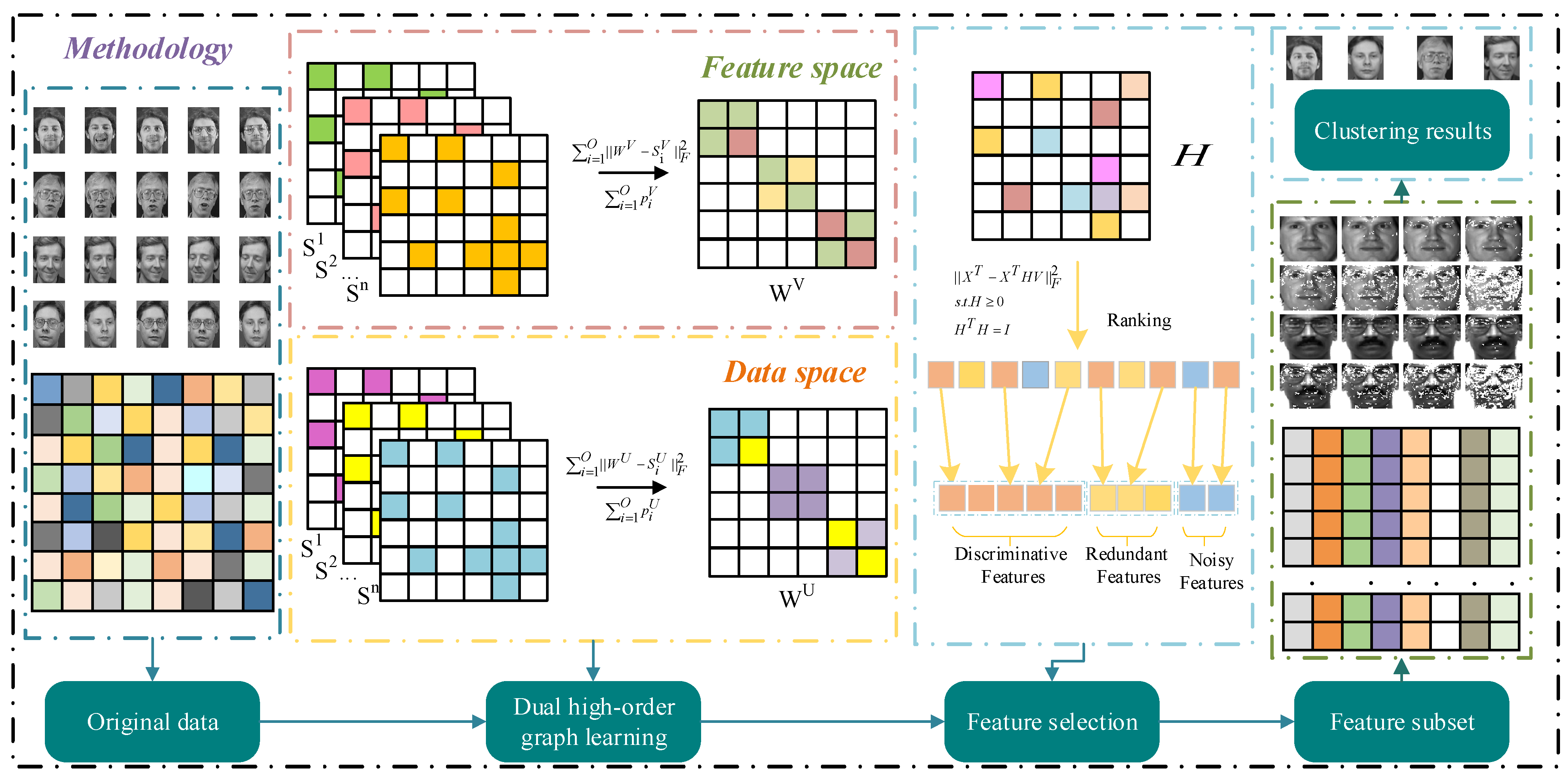
3. Methodology
3.1. Dual High-Order Graph Learning
3.2. The Proposed Feature Selection Method
3.3. Comparison of Unsupervised Feature Selection Based on Subspace Learning
3.4. Optimization
3.4.1. Update V and H
- (1)
- Fix V and update H:
- (2)
- Fix H and update V:
3.4.2. Update pV and WV
- (1)
- Fix WV and update pV:
- (2)
- Fix pV and update WV:
3.5. Convergence Analysis
| Algorithm 1 The procedure of DHBWSL. |
| Input: Data matrix X ∈ Rd×n; Parameter β, γ, λ, σ and k; The number of selected features l; The maximum number of iterations NIter. Initialization: The iteration time t = 0; H = rand(d,l), V = rand(l,d), Il = eye(l), Construct the attribute score matrix Q; Repeat: 1. Update the feature selection matrix H with Equation (15). 2. Update coefficient matrix V with Equation (18). 3. Update by solving subproblem (20). 4. Update by solving subproblem (21). 5. Update WV by solving subproblem (39). 6. Update Wu by solving subproblem (40). Until Convergence Output: Index of selected features; New data matrix Xnew ∈ Rl×n. Feature selection: The score of d features is calculated according to ‖hi‖2, and the first l feature with the highest score is selected. |
4. Experiments
4.1. Datasets
4.2. Comparison Methods
4.3. Experimental Settings
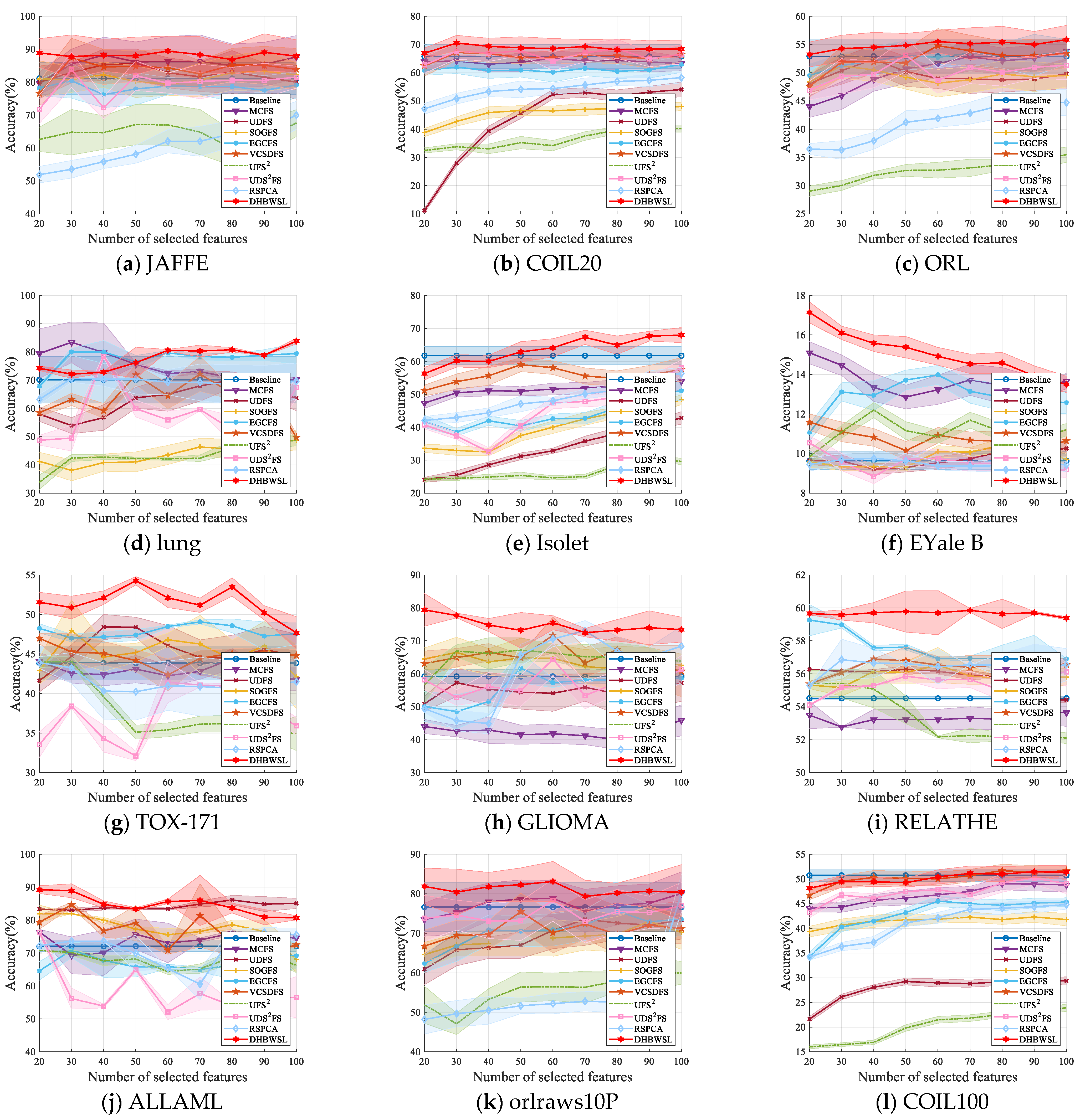
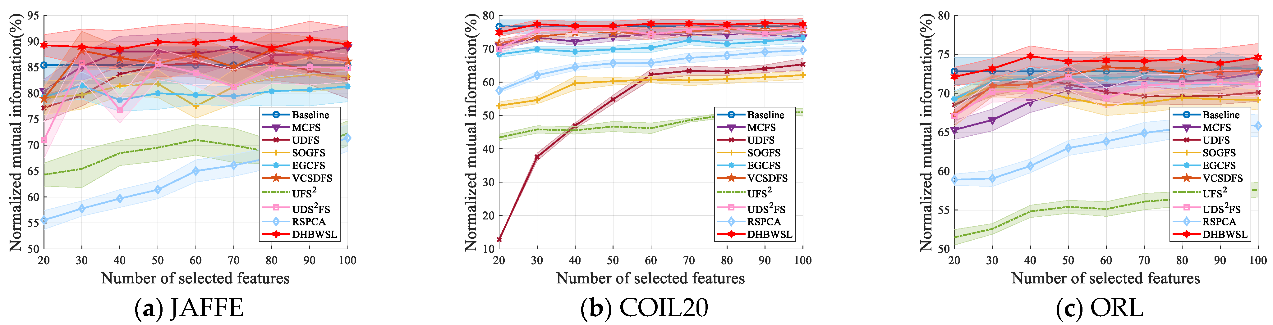
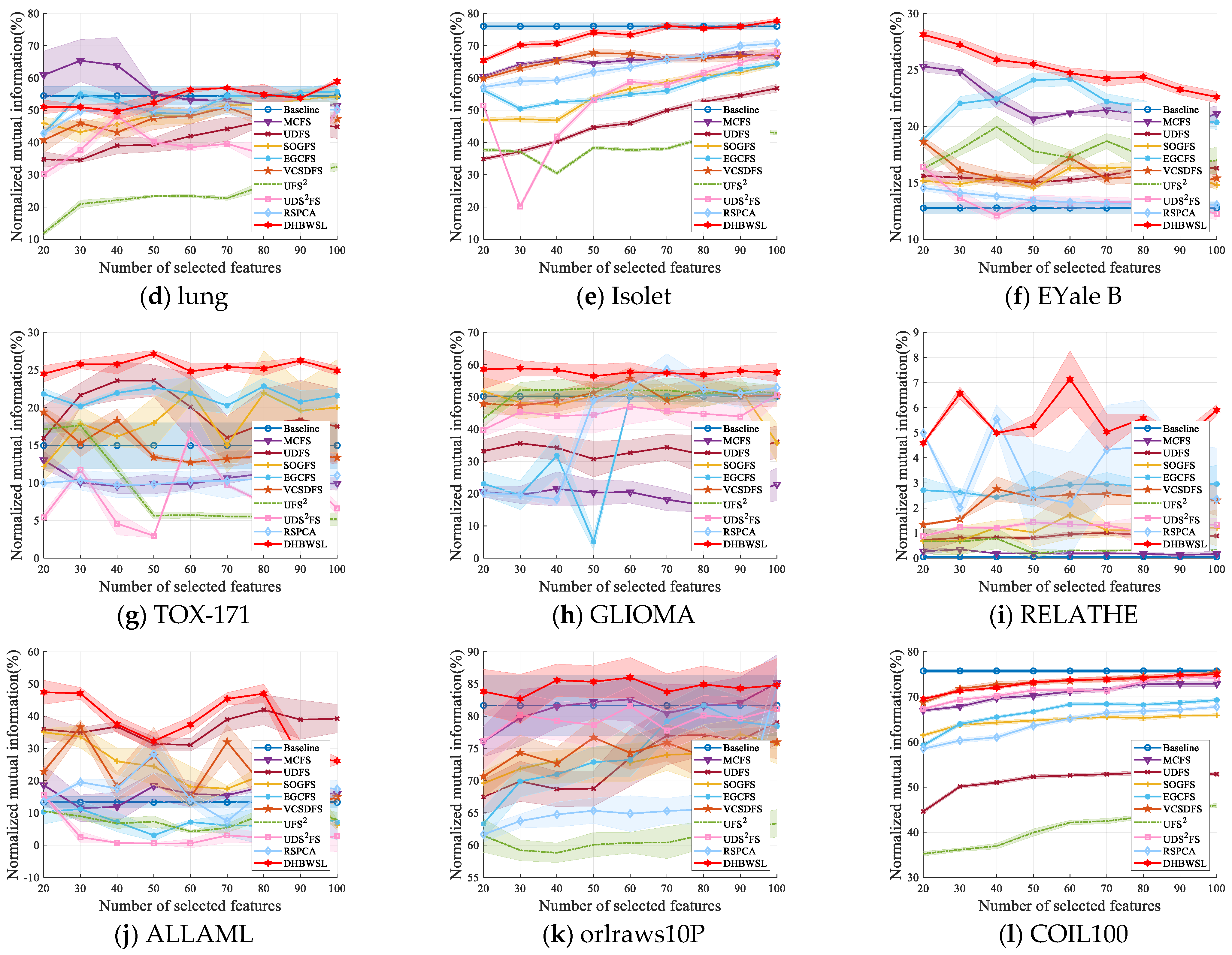
4.4. Clustering Results and Analysis

| Datasets | Baseline | MCFS | UDFS | SOGFS | EGCFS | VCSDFS | UFS2 | UDS2FS | RSPCA | DHBWSL |
|---|---|---|---|---|---|---|---|---|---|---|
| JAFFE | 81.10 ±4.85 (all) | 88.24 ±5.40 (40) | 85.77 ±4.31 (50) | 83.29 ±6.15 (90) | 80.40 ±5.29 (30) | 87.37 ±5.97 (30) | 67.58 ±4.06 (100) | 83.76 ±5.40 (30) | 69.95 ±4.23 (100) | 89.41 ±4.54 (60) |
| COIL20 | 65.75 ±4.16 (all) | 65.14 ±2.53 (60) | 54.05 ±2.63 (100) | 48.04 ±1.40 (100) | 62.98 ±2.87 (100) | 67.16 ±2.81 (30) | 40.25 ±1.18 (90) | 68.43 ±3.36 (80) | 58.26 ±1.85 (100) | 70.52 ±2.71 (30) |
| ORL | 52.90 ±3.08 (all) | 53.86 ±1.65 (100) | 52.39 ±2.48 (40) | 51.20 ±2.21 (30) | 53.73 ±2.18 (100) | 54.77 ±3.03 (60) | 35.49 ±1.35 (100) | 53.09 ±2.93 (50) | 44.73 ±2.05 (90) | 55.85 ±2.53 (100) |
| lung | 70.10 ±8.22 (all) | 83.42 ±7.23 (30) | 70.15 ±2.82 (80) | 48.67 ±3.42 (100) | 80.02 ±1.26 (30) | 72.17 ±6.20 (70) | 48.65 ±1.87 (100) | 78.47 ±0.70 (40) | 70.62 ±1.34 (30) | 83.82 ±1.03 (100) |
| Isolet | 61.73 ±2.77 (all) | 54.16 ±2.53 (90) | 42.83 ±1.89 (100) | 48.35 ±1.51 (100) | 51.07 ±2.93 (100) | 58.98 ±2.11 (50) | 30.44 ±1.27 (90) | 58.01 ±2.45 (100) | 56.28 ±1.89 (100) | 67.97 ±2.29 (100) |
| EYale B | 9.64 ±0.45 (all) | 15.10 ±0.56 (20) | 10.26 ±0.39 (100) | 10.42 ±0.35 (80) | 13.98 ±0.48 (60) | 11.59 ±0.41 (20) | 12.20 ±0.38 (40) | 10.54 ±0.35 (20) | 9.76 ±0.33 (40) | 17.14 ±0.53 (20) |
| TOX_171 | 43.86 ±2.17 (all) | 44.42 ±1.27 (80) | 48.42 ±1.59 (40) | 47.98 ±3.80 (70) | 49.06 ±0.26 (70) | 46.99 ±0.46 (20) | 44.06 ±0.58 (30) | 41.43 ±2.57 (60) | 43.92 ±0.73 (20) | 54.27 ±0.52 (50) |
| GLIOMA | 59.20 ±2.19 (all) | 45.90 ±4.70 (100) | 57.30 ±4.17 (30) | 66.50 ±4.58 (30) | 61.70 ±4.46 (50) | 71.70 ±5.44 (60) | 67.20 ±3.75 (50) | 64.40 ±5.05 (60) | 73.10 ±3.08 (70) | 79.40 ±4.95 (20) |
| RELATHE | 54.51 ±0.10 (all) | 53.72 ±0.76 (90) | 56.27 ±0.21 (50) | 56.53 ±1.07 (60) | 59.26 ±0.95 (20) | 56.90 ±0.03 (40) | 55.41 ±0.88 (30) | 56.11 ±0.81 (100) | 56.85 ±1.24 (30) | 59.85 ±0.12 (70) |
| ALLAML | 72.08 ±1.62 (all) | 76.39 ±0.78 (20) | 86.11 ±1.42 (80) | 81.94 ±2.60 (60) | 70.90 ±2.27 (30) | 84.65 ±0.71 (30) | 70.83 ±0.01 (20) | 76.25 ±0.62 (20) | 76.32 ±1.39 (90) | 89.24 ±1.18 (20) |
| orlraws10P | 76.60 ±6.17 (all) | 80.05 ±5.49 (100) | 73.55 ±6.60 (70) | 73.00 ±3.93 (90) | 75.60 ±5.08 (80) | 75.45 ±4.68 (50) | 60.00 ±2.87 (100) | 78.35 ±5.32 (60) | 80.20 ±4.81 (100) | 82.30 ±4.23 (50) |
| COIL100 | 50.72 ±1.30 (all) | 49.01 ±1.21 (80) | 29.39 ±0.61 (90) | 42.30 ±1.09 (90) | 45.49 ±1.12 (60) | 51.69 ±1.27 (80) | 23.93 ±0.74 (100) | 50.15 ±1.32 (90) | 44.80 ±0.93 (100) | 51.47 ±1.18 (90) |
| Datasets | Baseline | MCFS | UDFS | SOGFS | EGCFS | VCSDFS | UFS2 | UDS2FS | RSPCA | DHBWSL |
|---|---|---|---|---|---|---|---|---|---|---|
| JAFFE | 85.43 ±3.51 (all) | 88.88 ±4.03 (100) | 86.06 ±3.51 (80) | 83.58 ±3.26 (90) | 81.48 ±2.59 (30) | 88.44 ±3.20 (80) | 72.25 ±2.38 (100) | 85.79 ±3.36 (30) | 71.38 ±2.56 (100) | 90.48 ±2.40 (70) |
| COIL20 | 76.69 ±1.99 (all) | 74.42 ±1.50 (60) | 65.33 ±1.75 (100) | 62.12 ±1.20 (100) | 73.36 ±1.61 (100) | 75.84 ±1.31 (80) | 51.27 ±0.81 (90) | 76.60 ±1.75 (80) | 69.56 ±1.35 (100) | 77.67 ±1.09 (90) |
| ORL | 72.83 ±1.74 (all) | 72.61 ±1.13 (100) | 72.09 ±1.39 (40) | 70.88 ±1.37 (30) | 73.13 ±1.17 (100) | 73.34 ±1.63 (60) | 57.60 ±0.93 (100) | 72.06 ±1.56 (50) | 66.07 ±1.50 (90) | 74.77 ±1.31 (40) |
| lung | 54.47 ±2.84 (all) | 65.38 ±6.55 (30) | 46.72 ±1.36 (80) | 54.21 ±2.54 (100) | 55.80 ±2.69 (100) | 50.91 ±1.58 (70) | 32.46 ±1.26 (100) | 50.06 ±1.47 (100) | 50.97 ±2.24 (70) | 58.91 ±0.89 (100) |
| Isolet | 76.06 ±1.26 (all) | 67.43 ±0.92 (90) | 56.84 ±1.27 (100) | 64.37 ±0.71 (100) | 64.43 ±1.30 (100) | 67.74 ±1.09 (50) | 43.56 ±0.65 (90) | 68.11 ±1.46 (100) | 70.81 ±0.97 (100) | 77.75 ±0.76 (100) |
| EYale B | 12.77 ±0.52 (all) | 25.31 ±0.48 (20) | 16.46 ±0.47 (90) | 16.41 ±0.56 (80) | 24.20 ±0.60 (60) | 18.64 ±0.41 (20) | 19.95 ±0.95 (40) | 16.42 ±0.50 (20) | 14.54 ±0.24 (20) | 28.13 ±0.48 (20) |
| TOX_171 | 14.98 ±3.03 (all) | 13.03 ±1.19 (20) | 23.61 ±2.09 (50) | 22.20 ±1.74 (60) | 22.85 ±1.12 (80) | 19.40 ±0.66 (20) | 17.66 ±0.80 (30) | 16.54 ±0.82 (60) | 11.00 ±1.60 (100) | 27.16 ±0.46 (50) |
| GLIOMA | 50.20 ±1.60 (all) | 22.94 ±5.08 (100) | 36.05 ±4.99 (100) | 52.37 ±3.62 (90) | 51.23 ±1.53 (90) | 55.72 ±3.37 (60) | 52.75 ±1.91 (50) | 50.68 ±2.39 (100) | 58.60 ±4.82 (70) | 58.89 ±2.40 (30) |
| RELATHE | 0.05 ±0.02 (all) | 0.35 ±0.01 (30) | 1.01 ±0.09 (70) | 1.73 ±0.95 (60) | 2.96 ±0.75 (100) | 2.76 ±0.49 (40) | 0.79 ±0.41 (40) | 1.43 ±0.09 (50) | 5.54 ±0.57 (40) | 7.14 ±1.12 (60) |
| ALLAML | 13.33 ±1.84 (all) | 18.63 ±6.11 (30) | 41.97 ±4.63 (80) | 34.99 ±1.24 (20) | 11.22 ±2.39 (100) | 36.68 ±2.05 (30) | 10.94 ±2.20 (90) | 15.58 ±0.62 (20) | 28.40 ±5.96 (50) | 47.42 ±3.72 (20) |
| orlraws10P | 81.76 ±4.70 (all) | 85.17 ±4.34 (100) | 79.05 ±3.36 (100) | 77.19 ±2.37 (90) | 81.69 ±3.14 (80) | 76.69 ±3.04 (50) | 63.29 ±2.13 (100) | 81.59 ±3.00 (60) | 84.77 ±3.04 (100) | 85.34 ±2.48 (50) |
| COIL100 | 75.73 ±0.34 (all) | 72.88 ±0.6 (100) | 53.15 ±0.53 (80) | 65.91 ±0.37 (100) | 69.29 ±0.36 (100) | 74.51 ±0.54 (80) | 45.97 ±0.46 (100) | 74.42 ±0.50 (90) | 67.78 ±0.40 (100) | 74.95 ±6.30 (100) |
| Datasets | Baseline | MCFS | UDFS | SOGFS | EGCFS | VCSDFS | UFS2 | UDS2FS | RSPCA | DHBWSL |
|---|---|---|---|---|---|---|---|---|---|---|
| JAFFE | 0.06 | 0.86 | 1.48 | 4.40 | 1.12 | 0.38 | 1.59 | 1.52 | 0.73 | 1.32 |
| COIL20 | 0.47 | 6.64 | 13.94 | 96.53 | 19.71 | 1.28 | 14.82 | 5.85 | 1.38 | 10.91 |
| ORL | 0.18 | 2.03 | 2.79 | 7.96 | 3.51 | 1.24 | 3.37 | 3.13 | 1.19 | 4.18 |
| lung | 2.75 | 6.04 | 68.34 | 2408.09 | 93.14 | 8.96 | 5.24 | 41.52 | 27.92 | 30.28 |
| Isolet | 0.46 | 7.07 | 13.41 | 23.73 | 18.86 | 1.40 | 11.24 | 1.68 | 0.77 | 8.89 |
| EYale B | 1.45 | 3.26 | 24.92 | 65.17 | 58.57 | 1.43 | 46.04 | 2.59 | 1.68 | 34.10 |
| TOX_171 | 25.18 | 1.28 | 873.81 | 2834.97 | 1242.36 | 27.17 | 17.83 | 180.34 | 135.95 | 405.69 |
| GLIOMA | 12.39 | 0.89 | 607.04 | 2314.70 | 597.92 | 16.81 | 3.72 | 87.42 | 36.44 | 245.35 |
| RELATHE | 11.42 | 11.86 | 418.58 | 944.73 | 579.20 | 16.57 | 37.48 | 143.23 | 62.56 | 338.26 |
| ALLAML | 47.20 | 6.75 | 1298.96 | 10,709.38 | 1145.44 | 132.98 | 7.40 | 453.89 | 149.60 | 243.76 |
| orlraws10P | 163.67 | 15.68 | 2566.06 | 19,028.84 | 4159.70 | 87.63 | 22.62 | 805.71 | 451.26 | 1746.03 |
| COIL100 | 45.42 | 31.35 | 320.69 | 962.12 | 2015.05 | 1.33 | 88.20 | 12.67 | 11.09 | 311.45 |
| Datasets | Baseline | MCFS | UDFS | SOGFS | EGCFS | VCSDFS | UFS2 | UDS2FS | RSPCA | |
|---|---|---|---|---|---|---|---|---|---|---|
| JAFFE | p h | 0.0033 1 | 4.9999 × 10⁻⁹ 1 | 1.1243 × 10⁻¹¹ 1 | 7.6029 × 10⁻¹⁶ 1 | 0.0088 1 | 8.1090 × 10⁻⁴ 1 | 1.7584 × 10⁻¹⁸ 1 | 6.6927 × 10⁻⁵ 1 | 2.7192 × 10⁻¹⁰ 1 |
| COIL20 | p h | 0.0083 1 | 2.2206 × 10⁻⁷ 1 | 2.7762 × 10⁻²⁹ 1 | 2.1609 × 10−44 1 | 3.2358 × 10⁻³⁵ 1 | 1.8528 × 10⁻⁶ 1 | 7.8998 × 10−41 1 | 0.0109 1 | 2.0050 × 10⁻¹⁷ 1 |
| ORL | p h | 4.1188 × 10⁻⁴ 1 | 6.1222 × 10⁻⁷ 1 | 1.6053 × 10⁻¹¹ 1 | 9.9364 × 10⁻⁵ 1 | 0.0046 1 | 0.2030 0 | 5.2170 × 10⁻²⁸ 1 | 2.5978 × 10⁻⁵ 1 | 2.4171 × 10⁻¹⁶ 1 |
| lung | p h | 1.7868 × 10⁻⁷ 1 | 1.4484 × 10⁻¹⁶ 1 | 2.9665 × 10⁻⁸ 1 | 1.7777 × 10⁻¹² 1 | 9.0574 × 10⁻²³ 1 | 0.0356 1 | 3.4934 × 10⁻¹⁹ 1 | 1.8391 × 10⁻⁶ 1 | 5.7823 × 10⁻¹⁰ 1 |
| Isolet | p h | 5.9167 × 10⁻²⁸ 1 | 2.1798 × 10⁻¹⁴ 1 | 2.7699 × 10⁻²⁵ 1 | 1.9143 × 10−36 1 | 1.4784 × 10⁻³⁵ 1 | 1.4844 × 10⁻¹¹ 1 | 5.9769 × 10−40 1 | 2.9701 × 10⁻⁷ 1 | 7.7368 × 10⁻¹⁹ 1 |
| EYale B | p h | 1.6388 × 10⁻²⁹ 1 | 1.0569 × 10⁻⁸ 1 | 1.4683 × 10⁻²⁸ 1 | 2.1944 × 10−41 1 | 2.6630 × 10⁻³² 1 | 9.4853 × 10⁻³¹ 1 | 1.6083 × 10⁻²⁶ 1 | 4.4488 × 10⁻²⁴ 1 | 4.5104 × 10⁻³⁵ 1 |
| TOX_171 | p h | 3.8869 × 10⁻⁶ 1 | 0.0093 1 | 1.7762 × 10⁻⁶ 1 | 4.5149 × 10⁻¹⁶ 1 | 5.0969 × 10⁻¹¹ 1 | 4.9939 × 10⁻⁹ 1 | 6.9265 × 10⁻¹³ 1 | 5.2356 × 10⁻⁹ 1 | 0.0219 1 |
| GLIOMA | p h | 4.3778 × 10⁻¹³ 1 | 7.9113 × 10⁻²⁶ 1 | 7.3934 × 10⁻²² 1 | 7.5027 × 10⁻¹⁴ 1 | 2.8855 × 10⁻²³ 1 | 9.1073 × 10⁻¹⁷ 1 | 2.4122 × 10⁻¹⁶ 1 | 6.6404 × 10⁻⁸ 1 | 7.1229 × 10⁻¹⁸ 1 |
| RELATHE | p h | 0.0371 1 | 5.2259 × 10−45 1 | 1.9256 × 10−81 1 | 4.8465 × 10−65 1 | 1.2509 × 10−74 1 | 6.0813 × 10⁻⁷ 1 | 3.2163 × 10−65 1 | 5.9863 × 10⁻¹⁰ 1 | 0.0069 1 |
| ALLAML | p h | 2.0298 × 10−37 1 | 6.0648 × 10⁻²⁰ 1 | 2.9455 × 10−51 1 | 1.3964 × 10−49 1 | 1.1054 × 10⁻⁹ 1 | 5.1027 × 10⁻¹⁶ 1 | 5.5017 × 10⁻³⁴ 1 | 5.9833 × 10−64 1 | 2.2404 × 10⁻³⁰ 1 |
| orlraws10P | p h | 5.5865 × 10⁻¹⁸ 1 | 1.5253 × 10⁻²¹ 1 | 5.3369 × 10⁻¹³ 1 | 1.6683 × 10⁻¹⁷ 1 | 1.3257 × 10⁻¹⁵ 1 | 1.1109 × 10⁻¹¹ 1 | 2.3574 × 10⁻¹⁵ 1 | 1.2112 × 10⁻¹⁹ 1 | 9.2441 × 10⁻¹⁸ 1 |
| COIL100 | p h | 1.9101 × 10⁻²¹ 1 | 1.0699 × 10⁻¹⁵ 1 | 1.1474 × 10−45 1 | 3.6026 × 10⁻¹³ 1 | 5.8528 × 10⁻²⁶ 1 | 3.1366 × 10⁻²³ 1 | 4.8302 × 10−49 1 | 1.1606 × 10⁻¹⁴ 1 | 3.6670 × 10⁻³² 1 |
| Datasets | Baseline | MCFS | UDFS | SOGFS | EGCFS | VCSDFS | UFS2 | UDS2FS | RSPCA | |
|---|---|---|---|---|---|---|---|---|---|---|
| JAFFE | p h | 5.0954 × 10⁻⁹ 1 | 4.5287 × 10⁻¹⁴ 1 | 1.2985 × 10⁻¹⁸ 1 | 2.1976 × 10⁻²⁵ 1 | 4.3009 × 10⁻⁷ 1 | 1.7813 × 10⁻⁵ 1 | 4.0952 × 10⁻¹⁸ 1 | 5.8906 × 10⁻¹⁰ 1 | 3.4081 × 10⁻¹⁶ 1 |
| COIL20 | p h | 0.9210 0 | 1.8565 × 10⁻¹¹ 1 | 8.3184 × 10⁻³⁵ 1 | 7.7725 × 10−54 1 | 1.3827 × 10−42 1 | 1.5602 × 10⁻¹² 1 | 2.1203 × 10−48 1 | 0.1891 0 | 1.5006 × 10⁻²⁶ 1 |
| ORL | p h | 1.3472 × 10⁻⁶ 1 | 3.8923 × 10⁻⁶ 1 | 4.2445 × 10⁻¹⁷ 1 | 7.9821 × 10⁻⁹ 1 | 1.1772 × 10⁻⁵ 1 | 0.1182 0 | 1.1551 × 10−37 1 | 6.1003 × 10⁻⁶ 1 | 9.6748 × 10⁻²³ 1 |
| lung | p h | 2.4998 × 10⁻¹⁸ 1 | 1.4410 × 10⁻²⁰ 1 | 2.0524 × 10⁻⁸ 1 | 2.4254 × 10⁻¹⁴ 1 | 2.1454 × 10⁻²⁴ 1 | 3.2489 × 10⁻⁷ 1 | 1.5531 × 10⁻²⁰ 1 | 3.3657 × 10⁻⁶ 1 | 6.0400 × 10⁻¹⁶ 1 |
| Isolet | p h | 6.9752 × 10−38 1 | 5.3449 × 10⁻²² 1 | 3.7346 × 10−36 1 | 5.3022 × 10−43 1 | 8.5538 × 10−47 1 | 7.4706 × 10⁻⁸ 1 | 2.4377 × 10−53 1 | 0.0243 1 | 7.7473 × 10⁻³⁰ 1 |
| EYale B | p h | 7.9018 × 10−44 1 | 7.7974 × 10⁻⁷ 1 | 4.9514 × 10⁻³⁵ 1 | 4.1198 × 10−45 1 | 6.5993 × 10−40 1 | 7.0041 × 10−42 1 | 2.5865 × 10⁻²⁸ 1 | 3.1037 × 10−37 1 | 1.0691 × 10−47 1 |
| TOX_171 | p h | 1.2300 × 10⁻¹⁵ 1 | 1.0453 × 10⁻⁴ 1 | 0.0275 1 | 1.8397 × 10⁻²² 1 | 1.1552 × 10⁻²⁶ 1 | 9.4111 × 10⁻¹⁸ 1 | 6.4780 × 10⁻²¹ 1 | 4.0051 × 10⁻¹² 1 | 0.0073 1 |
| GLIOMA | p h | 1.5787 × 10⁻⁴ 1 | 2.1801 × 10⁻³¹ 1 | 1.1535 × 10⁻³² 1 | 3.4468 × 10⁻¹⁴ 1 | 7.5197 × 10⁻³⁴ 1 | 4.1431 × 10⁻⁷ 1 | 1.7450 × 10⁻²⁰ 1 | 0.0239 1 | 5.2694 × 10⁻⁶ 1 |
| RELATHE | p h | 0.0153 1 | 1.1618 × 10−74 1 | 1.0218 × 10−93 1 | 1.2836 × 10−55 1 | 5.8358 × 10−90 1 | 2.2538 × 10⁻⁷ 1 | 3.5715 × 10−53 1 | 6.3098 × 10⁻⁸ 1 | 5.7191 × 10⁻¹³ 1 |
| ALLAML | p h | 2.4430 × 10⁻³¹ 1 | 5.4551 × 10⁻¹⁹ 1 | 4.3531 × 10−39 1 | 1.8018 × 10−62 1 | 5.2290 × 10⁻⁵ 1 | 1.7163 × 10⁻¹¹ 1 | 1.3913 × 10⁻²⁴ 1 | 8.8682 × 10−95 1 | 1.7695 × 10⁻²⁵ 1 |
| orlraws10P | p h | 2.8720 × 10⁻²² 1 | 2.2141 × 10⁻²⁵ 1 | 2.8931 × 10⁻¹⁷ 1 | 2.6862 × 10⁻¹⁸ 1 | 2.1888 × 10⁻¹⁷ 1 | 3.8995 × 10⁻¹⁴ 1 | 5.8639 × 10⁻⁶ 1 | 1.4837 × 10⁻²³ 1 | 9.1751 × 10⁻²¹ 1 |
| COIL100 | p h | 2.1942 × 10−40 1 | 7.4485 × 10⁻³¹ 1 | 1.7060 × 10−56 1 | 3.3267 × 10⁻²⁸ 1 | 2.7279 × 10−38 1 | 5.0523 × 10⁻³³ 1 | 1.9495 × 10−60 1 | 2.0572 × 10⁻³³ 1 | 9.8478 × 10−42 1 |
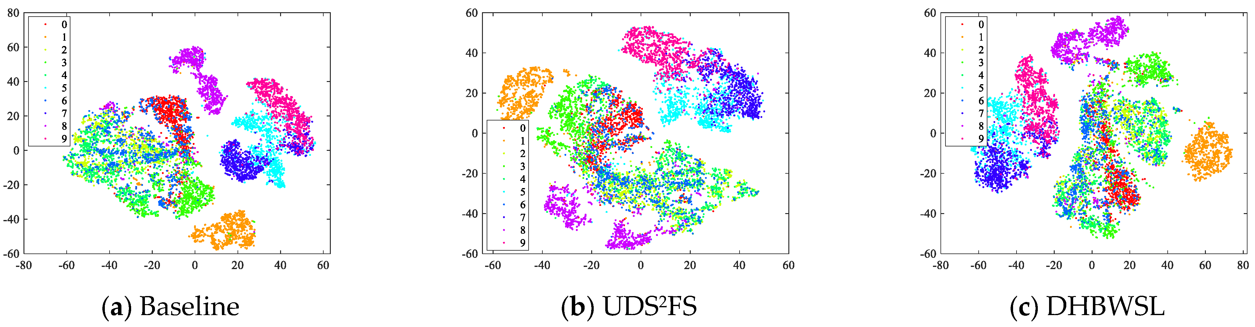
4.5. Visualization on Fashion MNIST
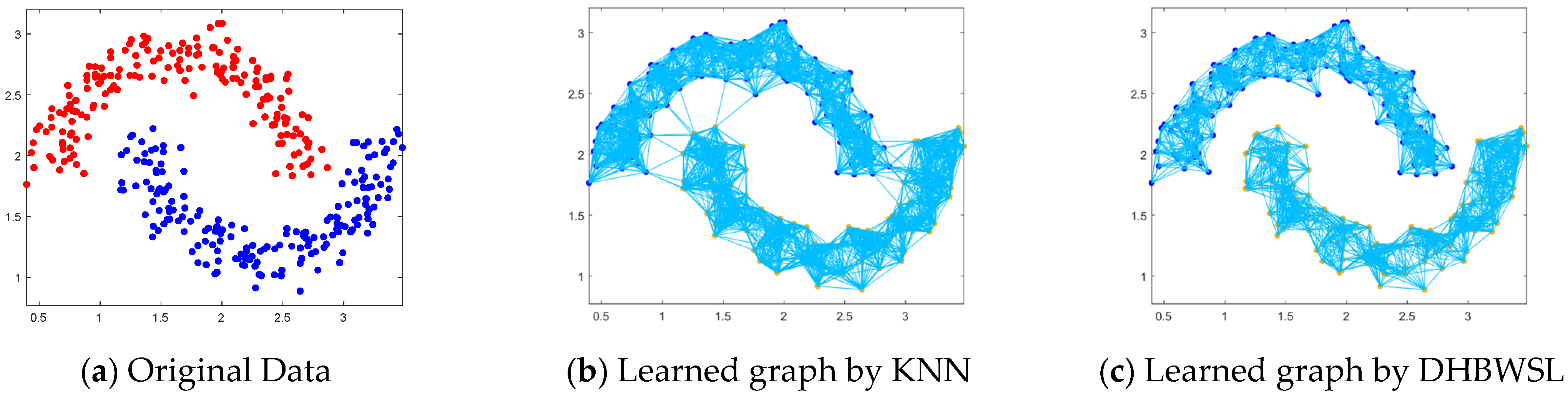
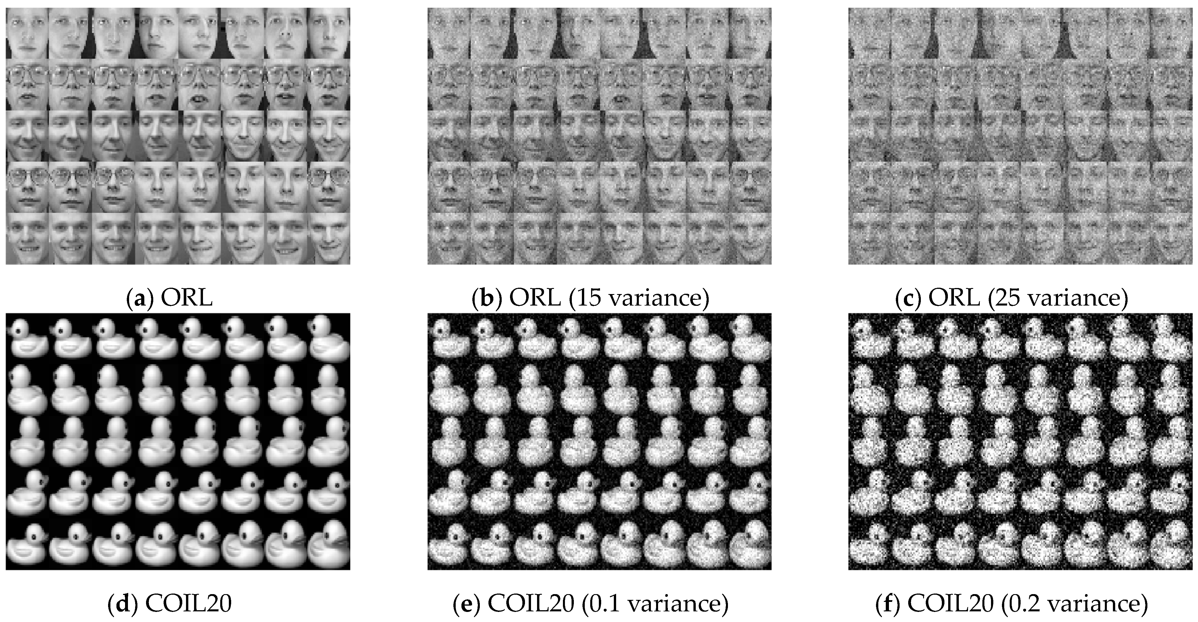
4.6. Two-Moon Dataset and Noise Test
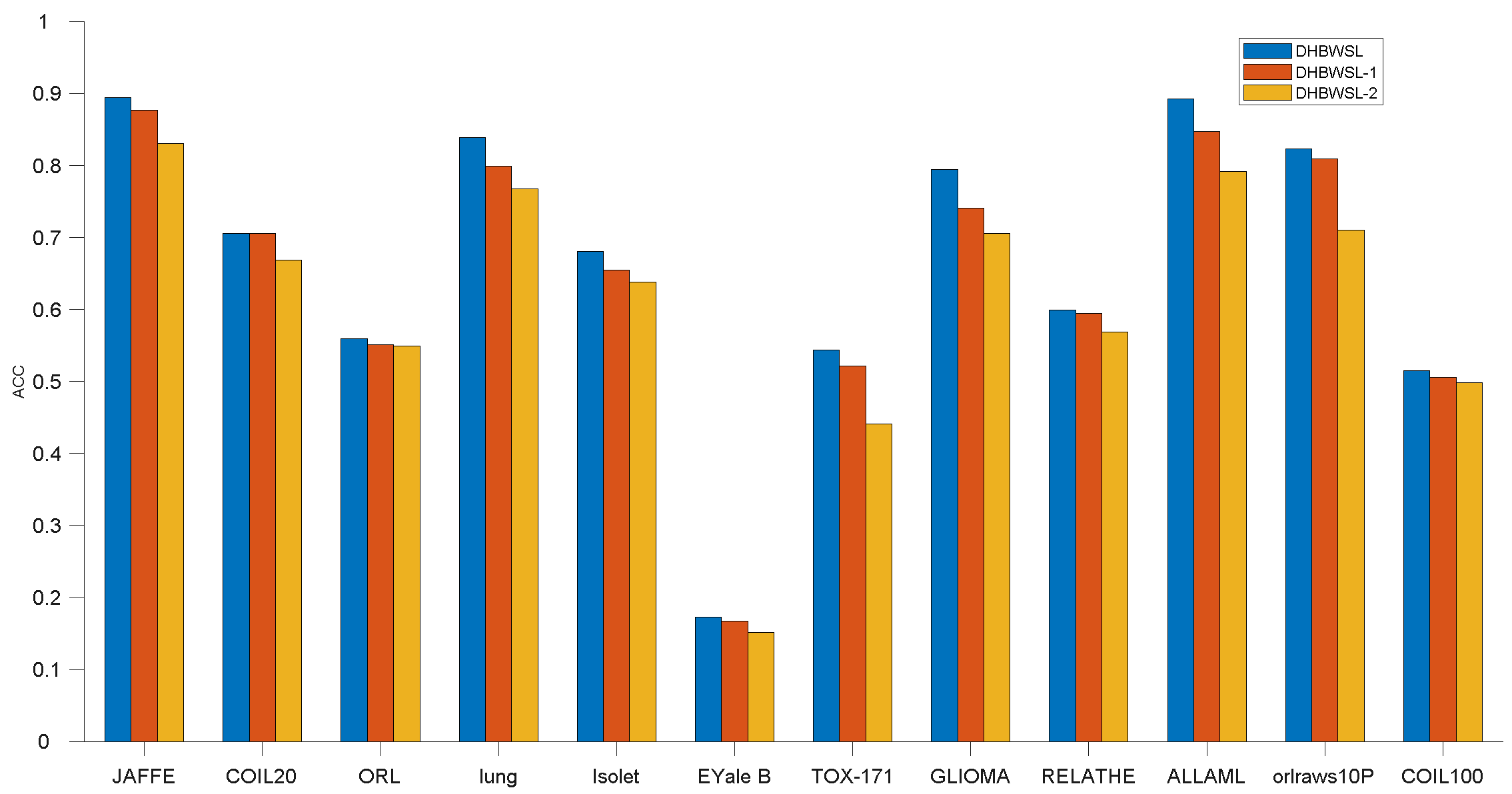
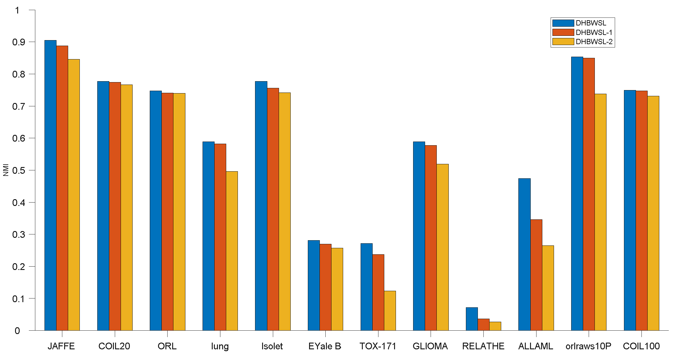
4.7. Ablation Study
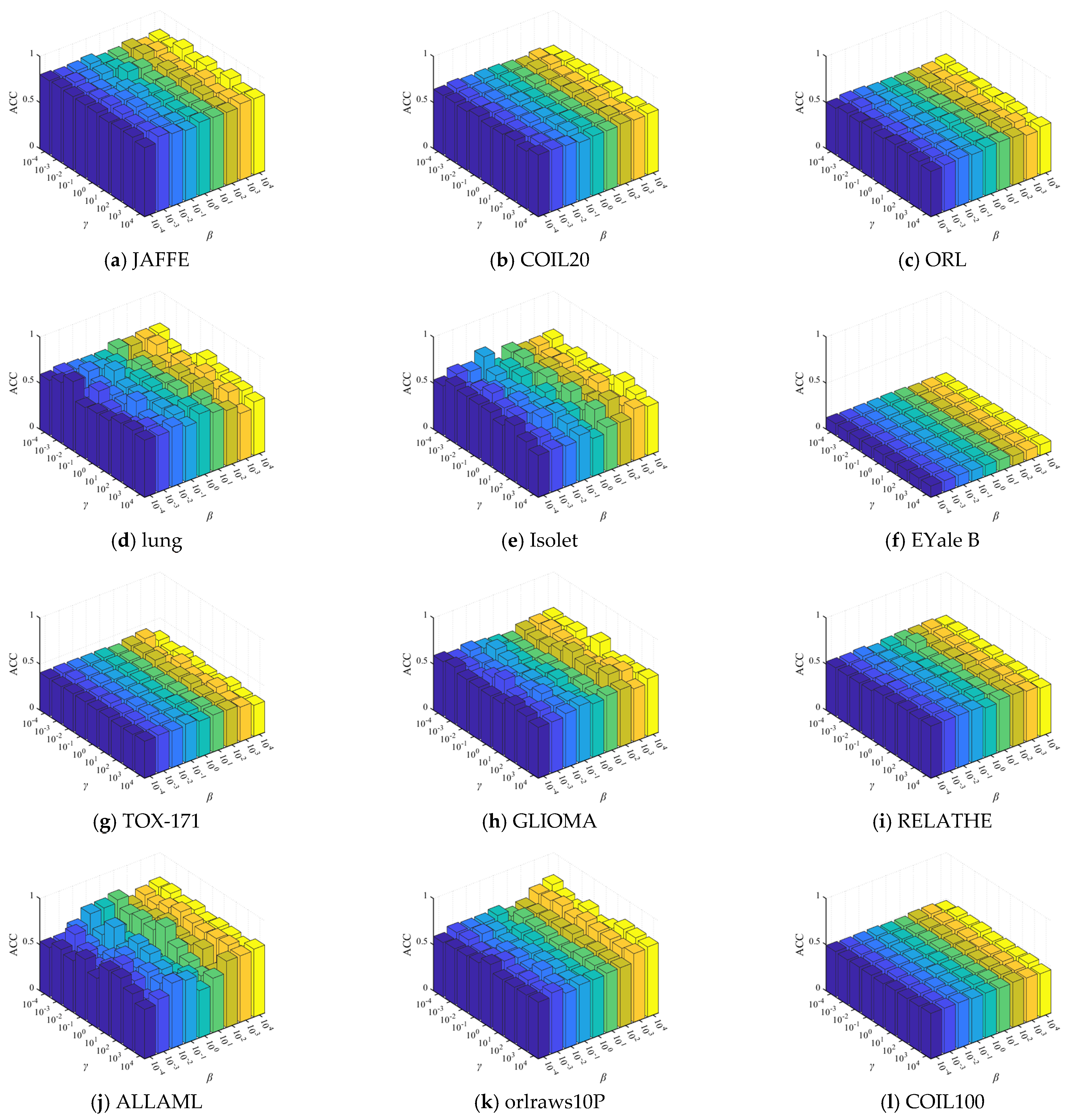
4.8. Parameters Sensitivity Analysis
4.9. Convergence Analysis and Computational Performance
5. Conclusions
Author Contributions
Funding
Institutional Review Board Statement
Data Availability Statement
Conflicts of Interest
References
- Wang, C.; Wang, J.; Gu, Z.; Wei, J.; Liu, J. Unsupervised feature selection by learning exponential weights. Pattern Recognit. 2024, 148, 0031–3203. [Google Scholar] [CrossRef]
- Tang, C.; Wang, J.; Zheng, X.; Liu, X.; Xie, W.; Li, X. Spatial and Spectral Structure Preserved Self-Representation for Unsupervised Hyperspectral Band Selection. IEEE Trans. Geosci. Remote Sens. 2023, 61, 5531413. [Google Scholar] [CrossRef]
- Guo, Y.; Sun, Y.; Wang, Z.; Nie, F.; Wang, F. Double-Structured Sparsity Guided Flexible Embedding Learning for Unsupervised Feature Selection. IEEE Trans. Neural Netw. Learn. Syst. 2023, 35, 13354–13367. [Google Scholar] [CrossRef]
- Wang, Z.; Li, Q.; Nie, F.; Wang, R.; Wang, F.; Li, X. Efficient Local Coherent Structure Learning via Self-Evolution Bipartite Graph. IEEE Trans. Cybern. 2024, 54, 4527–4538. [Google Scholar] [CrossRef]
- Lai, Z.; Chen, F.; Wen, J. Multi-view robust regression for feature extraction. Pattern Recognit. 2024, 149, 110219. [Google Scholar] [CrossRef]
- Niu, X.; Zhang, C.; Ma, Y.; Hu, L.; Zhang, J. A multi-view subspace representation learning approach powered by subspace transformation relationship. Knowl.-Based Syst. 2023, 277, 110816. [Google Scholar] [CrossRef]
- Wang, Z.; Wu, D.; Wang, R.; Nie, F.; Wang, F. Joint Anchor Graph Embedding and Discrete Feature Scoring for Unsupervised Feature Selection. IEEE Trans. Neural Netw. Learn. Syst. 2024, 35, 7974–7987. [Google Scholar] [CrossRef] [PubMed]
- Wen, J.; Fang, X.; Cui, J.; Fei, L.; Yan, K.; Chen, Y.; Xu, Y. Robust Sparse Linear Discriminant Analysis. IEEE Trans. Circuits Syst. Video Technol. 2019, 29, 390–403. [Google Scholar] [CrossRef]
- Greenacre, M.; Groenen, P.; Hastie, T.; D’Enza, A.; Markos, A.; Tuzhilina, E. Principal component analysis. Nat. Rev. Methods Primers 2022, 2, 100. [Google Scholar] [CrossRef]
- Kokiopoulou, E.; Saad, Y. Orthogonal Neighborhood Preserving Projections: A Projection-Based Dimensionality Reduction Technique. IEEE Trans. Pattern Anal. Mach. Intell. 2007, 29, 2143–2156. [Google Scholar] [CrossRef]
- Wu, H.; Wu, N. When Locally Linear Embedding Hits Boundary. J. Mach. Learn. Res. 2023, 24, 1–80. Available online: https://jmlr.org/papers/v24/21-0697.html (accessed on 3 August 2023).
- Xu, S.; Muselet, D.; Trémeau, A. Sparse coding and normalization for deep Fisher score representation. Comput. Vis. Image Underst. 2022, 220, 103436. [Google Scholar] [CrossRef]
- Nie, F.; Xiang, S.; Jia, Y.; Zhang, C.; Yan, S. Trace Ratio Criterion for Feature Selection. In Proceedings of the AAAI Conference on Artificial Intelligence, Chicago, IL, USA, 13–17 July 2008; Available online: https://api.semanticscholar.org/CorpusID:11957383 (accessed on 3 August 2023).
- Chandra, B.; Sharma, R. Deep learning with adaptive learning rate using laplacian score. Expert Syst. Appl. 2016, 63, 1–7. [Google Scholar] [CrossRef]
- Cai, D.; Zhang, C.; He, X. Unsupervised feature selection for multi-cluster data. In Proceedings of the 16th ACM SIGKDD International Conference on Knowledge Discovery and Data Mining, Washington, DC, USA, 24–28 July 2010; Volume 10, pp. 333–342. [Google Scholar] [CrossRef]
- Wang, Z.; Nie, F.; Wang, H.; Huang, H.; Wang, F. Toward Robust Discriminative Projections Learning Against Adversarial Patch Attacks. IEEE Trans. Neural Netw. Learn. Syst. 2024, 35, 18784–18798. [Google Scholar] [CrossRef] [PubMed]
- Wang, Z.; Nie, F.; Zhang, C.; Wang, R.; Li, X. Worst-Case Discriminative Feature Learning via Max-Min Ratio Analysis. IEEE Trans. Pattern Anal. Mach. Intell. 2024, 46, 641–658. [Google Scholar] [CrossRef]
- Yu, W.; Bian, J.; Nie, F.; Wang, R.; Li, X. Unsupervised Subspace Learning With Flexible Neighboring. IEEE Trans. Neural Netw. Learn. Syst. 2023, 34, 2043–2056. [Google Scholar] [CrossRef]
- Wang, S.; Nie, F.; Wang, Z.; Wang, R.; Li, X. Outliers Robust Unsupervised Feature Selection for Structured Sparse Subspace. IEEE Trans. Knowl. Data Eng. 2024, 36, 1234–1248. [Google Scholar] [CrossRef]
- Wang, S.; Pedrycz, W.; Zhu, Q.; Zhu, W. Subspace learning for unsupervised feature selection via matrix factorization. Pattern Recognit. 2015, 48, 10–19. [Google Scholar] [CrossRef]
- Wang, S.; Pedrycz, W.; Zhu, Q.; Zhu, W. Unsupervised feature selection via maximum projection and minimum redundancy. Knowl.-Based Syst. 2015, 75, 19–29. [Google Scholar] [CrossRef]
- Zheng, W.; Yan, H.; Yang, J. Robust unsupervised feature selection by nonnegative sparse subspace learning. Neurocomputing 2019, 334, 156–171. [Google Scholar] [CrossRef]
- Wu, J.; Li, Y.; Gong, J.; Min, W. Collaborative and Discriminative Subspace Learning for unsupervised multi-view feature selection. Eng. Appl. Artif. Intell. 2024, 133, 108145. [Google Scholar] [CrossRef]
- Zhang, Y.; Wang, Q.; Gong, D.; Song, X. Nonnegative Laplacian embedding guided subspace learning for unsupervised feature selection. Pattern Recognit. 2019, 93, 337–352. [Google Scholar] [CrossRef]
- Mandanas, F.D.; Kotropoulos, C.L. Subspace Learning and Feature Selection via Orthogonal Mapping. IEEE Trans. Signal Process. 2020, 68, 1034–1047. [Google Scholar] [CrossRef]
- Wu, J.; Song, M.; Min, W.; Lai, J.; Zheng, W. Joint adaptive manifold and embedding learning for unsupervised feature selection. Pattern Recognit. 2021, 112, 107742. [Google Scholar] [CrossRef]
- Shang, R.; Wang, W.; Stolkin, R.; Jiao, L. Subspace learning-based graph regularized feature selection. Knowl.-Based Syst. 2016, 112, 152–165. [Google Scholar] [CrossRef]
- Shang, R.; Meng, Y.; Wang, W.; Shang, F.; Jiao, L. Local discriminative based sparse subspace learning for feature selection. Pattern Recognit. 2019, 92, 219–230. [Google Scholar] [CrossRef]
- Shang, R.; Xu, K.; Jiao, L. Subspace learning for unsupervised feature selection via adaptive structure learning and rank approximation. Neurocomputing 2020, 413, 72–84. [Google Scholar] [CrossRef]
- Wang, Z.; Yuan, Y.; Wang, R.; Nie, F.; Huang, Q.; Li, X. Pseudo-Label Guided Structural Discriminative Subspace Learning for Unsupervised Feature Selection. IEEE Trans. Neural Netw. Learn. Syst. 2023, 35, 18605–18619. [Google Scholar] [CrossRef]
- Nie, F.; Wang, X.; Jordan, M.; Huang, H. The Constrained Laplacian Rank algorithm for graph-based clustering. In Proceedings of the AAAI Conference on Artificial Intelligence, Phoenix, AZ, USA, 12–17 February 2016; 2016; Volume 8, pp. 1969–1976. [Google Scholar] [CrossRef]
- Fan, K. On a Theorem of Weyl Concerning Eigenvalues of Linear Transformations I. Proc. Natl. Acad. Sci. USA 1949, 35, 652–655. [Google Scholar] [CrossRef]
- Du, H.; Wang, Y.; Zhang, F.; Zhou, Y. Low-Rank Discriminative Adaptive Graph Preserving Subspace Learning. Neural Process. Lett. 2020, 52, 2127–2149. [Google Scholar] [CrossRef]
- Sheng, C.; Song, P.; Zhang, W.; Chen, D. Dual-graph regularized subspace learning based feature selection. Digit. Signal Process. 2021, 117, 103175. [Google Scholar] [CrossRef]
- Yin, W.; Ma, Z.; Liu, Q. Discriminative subspace learning via optimization on Riemannian manifold. Pattern Recognit. 2023, 139, 109450. [Google Scholar] [CrossRef]
- Liu, Z.; Ou, W.; Zhang, K.; Xiong, H. Robust manifold discriminative distribution adaptation for transfer subspace learning. Expert Syst. Appl. 2024, 238, 122117. [Google Scholar] [CrossRef]
- Feng, W.; Wang, Z.; Cao, X.; Cai, B.; Guo, W.; Ding, W. Discriminative sparse subspace learning with manifold regularization. Expert Syst. Appl. 2024, 249, 123831. [Google Scholar] [CrossRef]
- Tang, J.; Gao, Y.; Jia, S.; Feng, H. Robust clustering with adaptive order graph learning. Inf. Sci. 2023, 649, 119659. [Google Scholar] [CrossRef]
- Tang, C.; Zheng, X.; Zhang, W.; Liu, X.; Zhu, X.; Zhu, E. Unsupervised feature selection via multiple graph fusion and feature weight learning. Sci. China Inf. Sci. 2023, 66, 152101. [Google Scholar] [CrossRef]
- Xu, W.; Gong, Y. Document clustering by concept factorization. In Proceedings of the Annual International ACM SIGIR Conference on Research and Development in Information Retrieval, Sheffield, UK, 25–29 July 2004; Volume 8, pp. 202–209. [Google Scholar] [CrossRef]
- Lee, D.; Seung, H. Algorithms for non-negative matrix factorization. In Proceedings of the 13th International Conference on Neural Information Processing Systems, Denver, CO, USA, 27 November–2 December 2000; Volume 7, pp. 535–541. Available online: https://dl.acm.org/doi/10.5555/3008751.3008829 (accessed on 3 August 2023).
- Cao, Z.; Xie, X. Structure learning with consensus label information for multi-view unsupervised feature selection. Expert Syst. Appl. 2024, 238, 121893. [Google Scholar] [CrossRef]
- Yang, B.; Xue, Z.; Wu, J.; Zhang, X.; Nie, F.; Chen, B. Anchor-graph regularized orthogonal concept factorization for document clustering. Neurocomputing 2024, 11, 127173. [Google Scholar] [CrossRef]
- Yang, Y.; Shen, H.T.; Ma, Z.; Huang, Z.; Zhou, X. ℓ2,1-norm regularized discriminative feature selection for unsupervised learning. In Proceedings of the Twenty-Second International Joint Conference on Artificial Intelligence, Barcelona, Spain, 16–22 July 2011; Volume 6, pp. 1589–1594. Available online: https://dl.acm.org/doi/10.5555/2283516.2283660 (accessed on 3 August 2023).
- Nie, F.; Zhu, W.; Li, X. Unsupervised feature selection with structured graph optimization. In Proceedings of the Thirtieth AAAI Conference on Artificial Intelligence, Phoenix, AZ, USA, 12–17 February 2016; Volume 7, pp. 1302–1308. Available online: https://dl.acm.org/doi/10.5555/3015812.3016004 (accessed on 3 August 2023).
- Zhang, R.; Zhang, Y.; Li, X. Unsupervised Feature Selection via Adaptive Graph Learning and Constraint. IEEE Trans. Neural Netw. Learn. Syst. 2022, 33, 1355–1362. [Google Scholar] [CrossRef]
- Karami, S.; Saberi-Movahed, F.; Tiwari, P.; Marttinen, P.; Vahdati, S. Unsupervised feature selection based on variance–covariance subspace distance. Neural Netw. 2023, 166, 188–203. [Google Scholar] [CrossRef]
- Chang, H.; Guo, J.; Zhu, W. Rethinking Embedded Unsupervised Feature Selection: A Simple Joint Approach. IEEE Trans. Big Data 2023, 9, 380–387. [Google Scholar] [CrossRef]
- Chen, K.; Peng, Y.; Nie, F.; Kong, W. Soft Label Guided Unsupervised Discriminative Sparse Subspace Feature Selection. J. Classif. 2024, 41, 129–157. [Google Scholar] [CrossRef]
- Bian, J.; Zhao, D.; Nie, F.; Wang, R.; Li, X. Robust and Sparse Principal Component Analysis with Adaptive Loss Minimization for Feature Selection. IEEE Trans. Neural Netw. Learn. Syst. 2024, 35, 3601–3614. [Google Scholar] [CrossRef] [PubMed]


| Notations | Definition |
|---|---|
| X | The data matrix |
| H | The feature selection matrix |
| V | The coefficient matrix |
| n | The sample number |
| d | The feature quantity |
| l | The number of selected features |
| k | The number of nearest neighbors |
| c | The number of clusters |
| xi | The i-th row vector of matrix X |
| xj | The j-th column vector of matrix X |
| The feature Boolean variable | |
| WV | The feature adjacency matrix |
| DV | The feature graph degree matrix |
| LV | The feature Laplacian matrix |
| The data Boolean variable | |
| WU | The data adjacency matrix |
| DU | The data graph degree matrix |
| LU | The data Laplacian matrix |
| 1 | A column vector with all 1 s |
| Methods | High-Order Graph Learning | Minimum Redundant | Boolean Weight | Sparse Regularization | Orthogonal |
|---|---|---|---|---|---|
| MFFS [20] (2015) | × | × | × | × | √ |
| MPMR [21] (2015) | × | √ | × | × | √ |
| SGFS [27] (2016) | × | × | × | ℓ2,1-norm | √ |
| LDSSL [28] (2019) | × | × | × | ℓ1-norm | √ |
| LRDAGP [33] (2020) | × | × | × | ℓ2,1-norm | √ |
| DGSLFS [34] (2021) | × | × | × | ℓ2,1-norm | √ |
| USFN [18] (2023) | × | × | × | × | √ |
| MODA [35] (2023) | × | × | × | × | √ |
| RMDDA [36] (2024) | × | × | × | F-norm | √ |
| DSSL-MR [37] (2024) | × | × | × | ℓ2,1-norm | × |
| DHBWSL | √ | × | √ | ℓ2,1-norm | √ |
| Datasets | Instance | Feature | Class | Type |
|---|---|---|---|---|
| JAFFE | 213 | 676 | 10 | Face images |
| COIL20 | 1440 | 1024 | 20 | Object images |
| ORL | 400 | 1024 | 40 | Face images |
| lung | 203 | 3312 | 4 | Biological |
| Isolet | 1560 | 617 | 26 | Speech Signal |
| EYale B | 2414 | 1024 | 38 | Face images |
| TOX_171 | 171 | 5748 | 4 | Biological |
| GLIOMA | 50 | 4434 | 4 | Biological |
| RELATHE | 1427 | 4322 | 2 | Text |
| ALLAML | 72 | 7129 | 2 | Biological |
| orlraws10P | 100 | 10,304 | 10 | Face images |
| COIL100 | 7200 | 1024 | 100 | Object images |
| Noise Datasets | Accuracy (%) | ||||||||
|---|---|---|---|---|---|---|---|---|---|
| MCFS | UDFS | SOGFS | EGCFS | VCSDFS | UFS2 | UDS2FS | RSPCA | DHBWSL | |
| ORL (15 variance) | 51.94 ±2.59 (100) | 45.84 ±1.78 (40) | 49.89 ±2.57 (100) | 53.31 ±2.45 (80) | 50.99 ±3.04 (90) | 33.85 ±1.18 (100) | 50.66 ±2.09 (90) | 43.84 ±2.62 (100) | 53.36 ±2.30 (100) |
| ORL (25 variance) | 44.74 ±2.40 (100) | 45.01 ±2.37 (100) | 44.79 ±1.95 (100) | 49.45 ±2.50 (90) | 46.90 ±1.55 (90) | 31.54 ±1.08 (100) | 43.87 ±2.43 (90) | 41.30 ±2.30 (100) | 49.14 ±2.27 (100) |
| COIL20 (0.1 variance) | 64.91 ±2.67 (60) | 62.22 ±2.94 (100) | 61.76 ±3.13 (100) | 62.10 ±2.64 (80) | 67.45 ±2.24 (80) | 40.18 ±1.50 (100) | 67.81 ±2.42 (50) | 59.37 ±2.10 (100) | 69.19 ±1.82 (80) |
| COIL20 (0.2 variance) | 64.32 ±3.55 (100) | 62.82 ±2.80 (90) | 62.99 ±2.23 (100) | 62.41 ±1.72 (80) | 65.94 ±2.47 (50) | 37.56 ±0.99 (100) | 68.33 ±1.63 (90) | 58.76 ±2.03 (100) | 69.51 ±1.78 (90) |
| Noise datasets | Normalized Mutual Information (%) | ||||||||
| MCFS | UDFS | SOGFS | EGCFS | VCSDFS | UFS2 | UDS2FS | RSPCA | DHBWSL | |
| ORL (15 variance) | 71.19 ±1.39 (100) | 66.92 ±0.99 (40) | 70.02 ±1.09 (100) | 72.10 ±0.84 (100) | 70.25 ±1.77 (80) | 55.80 ±1.15 (100) | 70.52 ±1.37 (90) | 64.82 ±1.32 (100) | 72.14 ±1.06 (100) |
| ORL (25 variance) | 64.98 ±1.61 (100) | 64.44 ±0.97 (100) | 63.88 ±1.17 (100) | 68.46 ±0.93 (90) | 66.60 ±1.15 (90) | 53.21 ±1.03 (100) | 64.45 ±1.42 (90) | 62.18 ±1.25 (100) | 68.27 ±1.66 (90) |
| COIL20 (0.1 variance) | 75.10 ±0.86 (100) | 71.15 ±1.28 (100) | 72.15 ±1.07 (100) | 72.72 ±1.16 (70) | 76.28 ±0.95 (80) | 50.94 ±0.90 (100) | 76.80 ±1.40 (50) | 69.30 ±1.36 (100) | 77.41 ±1.17 (100) |
| COIL20 (0.2 variance) | 73.97 ±1.52 (100) | 70.87 ±1.27 (90) | 71.57 ±1.02 (80) | 71.45 ±1.11 (90) | 73.76 ±1.30 (80) | 46.87 ±0.77 (100) | 76.10 ±0.96 (90) | 68.90 ±1.18 (100) | 76.49 ±1.26 (80) |
| Algorithms | Computational Complexity |
|---|---|
| MCFS | O(t(dn2 + cl3 + cnl2 + dlogd)) |
| UDFS | O(t(d3)) |
| SOGFS | O(t(d3 + n3)) |
| EGCFS | O(t(n3 + dn + nl)) |
| VCSDFS | O(t(d2)) |
| UFS2 | O(t(ncd + ld)) |
| UDS2FS | O(t(d2lcn + dn2 + ln2)) |
| RSPCA | O(t(nd + max(dlk, dlogd, llogl, l3))) |
| DHBWSL | O(t(nd + d2 + n2 + ld2 + d2n + dl)) |
Disclaimer/Publisher’s Note: The statements, opinions and data contained in all publications are solely those of the individual author(s) and contributor(s) and not of MDPI and/or the editor(s). MDPI and/or the editor(s) disclaim responsibility for any injury to people or property resulting from any ideas, methods, instructions or products referred to in the content. |
© 2025 by the authors. Licensee MDPI, Basel, Switzerland. This article is an open access article distributed under the terms and conditions of the Creative Commons Attribution (CC BY) license (https://creativecommons.org/licenses/by/4.0/).
Share and Cite
Wei, Y.; Ma, J.; Ma, Z.; Huang, Y. Subspace Learning for Dual High-Order Graph Learning Based on Boolean Weight. Entropy 2025, 27, 107. https://doi.org/10.3390/e27020107
Wei Y, Ma J, Ma Z, Huang Y. Subspace Learning for Dual High-Order Graph Learning Based on Boolean Weight. Entropy. 2025; 27(2):107. https://doi.org/10.3390/e27020107
Chicago/Turabian StyleWei, Yilong, Jinlin Ma, Ziping Ma, and Yulei Huang. 2025. "Subspace Learning for Dual High-Order Graph Learning Based on Boolean Weight" Entropy 27, no. 2: 107. https://doi.org/10.3390/e27020107
APA StyleWei, Y., Ma, J., Ma, Z., & Huang, Y. (2025). Subspace Learning for Dual High-Order Graph Learning Based on Boolean Weight. Entropy, 27(2), 107. https://doi.org/10.3390/e27020107