

Information Geometry Theoretic Measures for Characterizing Neural Information Processing from Simulated EEG Signals


Abstract
1. Introduction
2. Methods
2.1. Stochastic Nonlinear Oscillator Models of EEG Signals
2.2. Initial Conditions (ICs) and Specifications of Stochastic Simulations
2.3. Information Geometry Theoretic Measures: Information Rate and Causal Information Rate
2.4. Shannon Differential Entropy and Transfer Entropy
3. Results
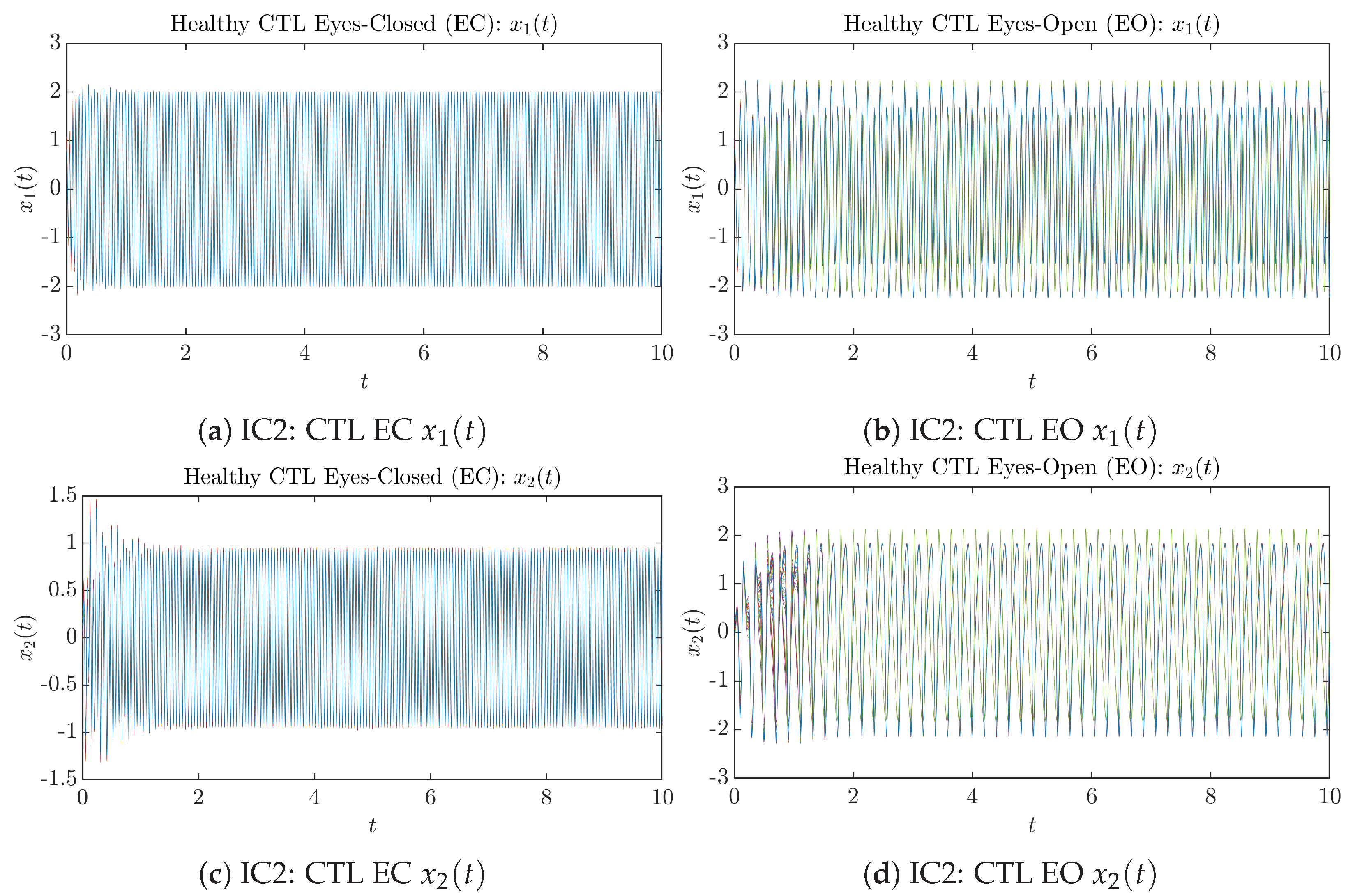
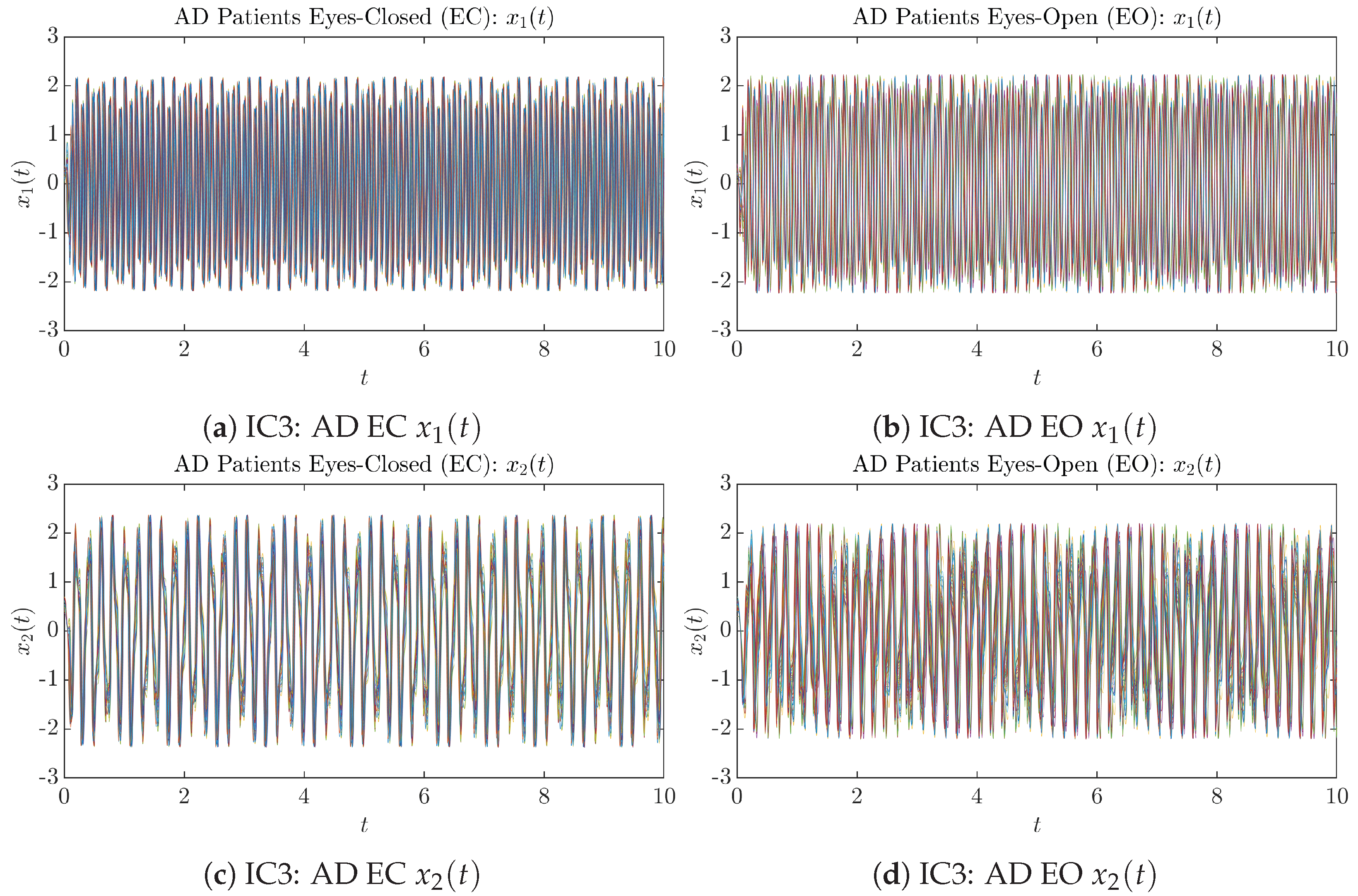
3.1. Sample Trajectories of and
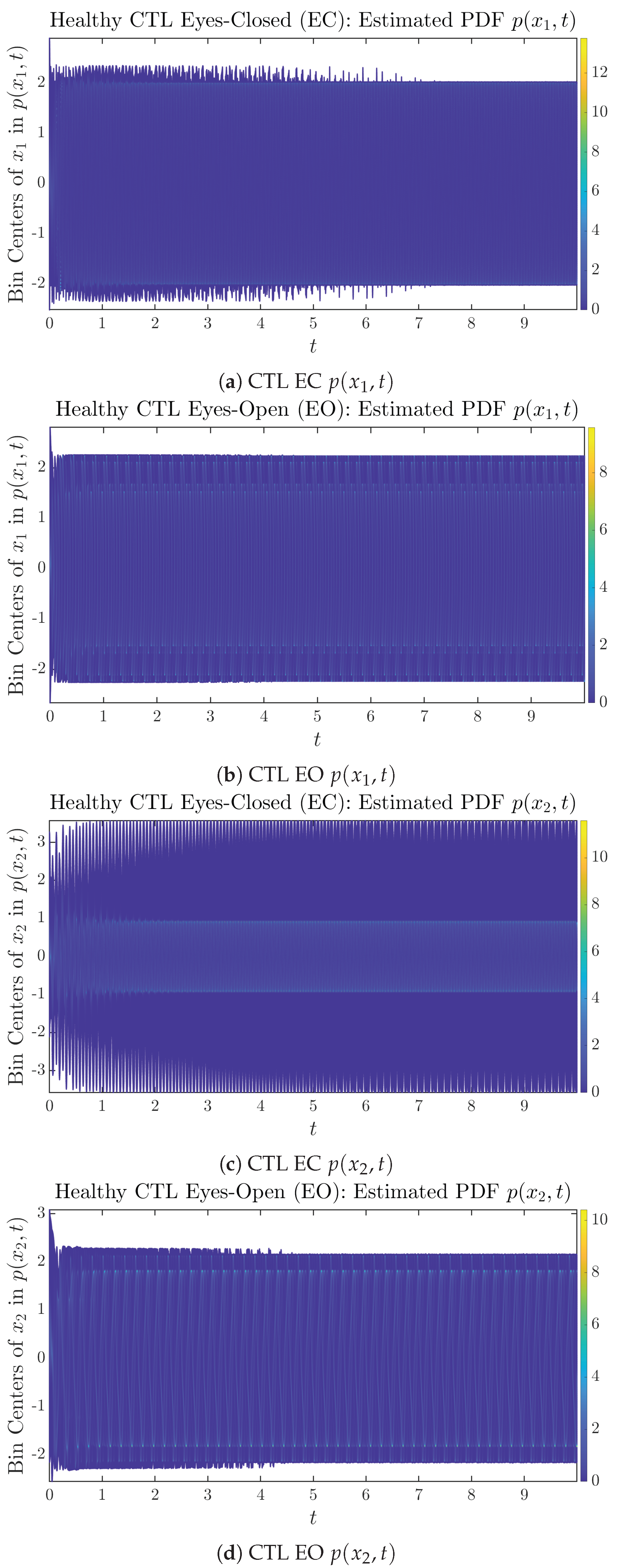
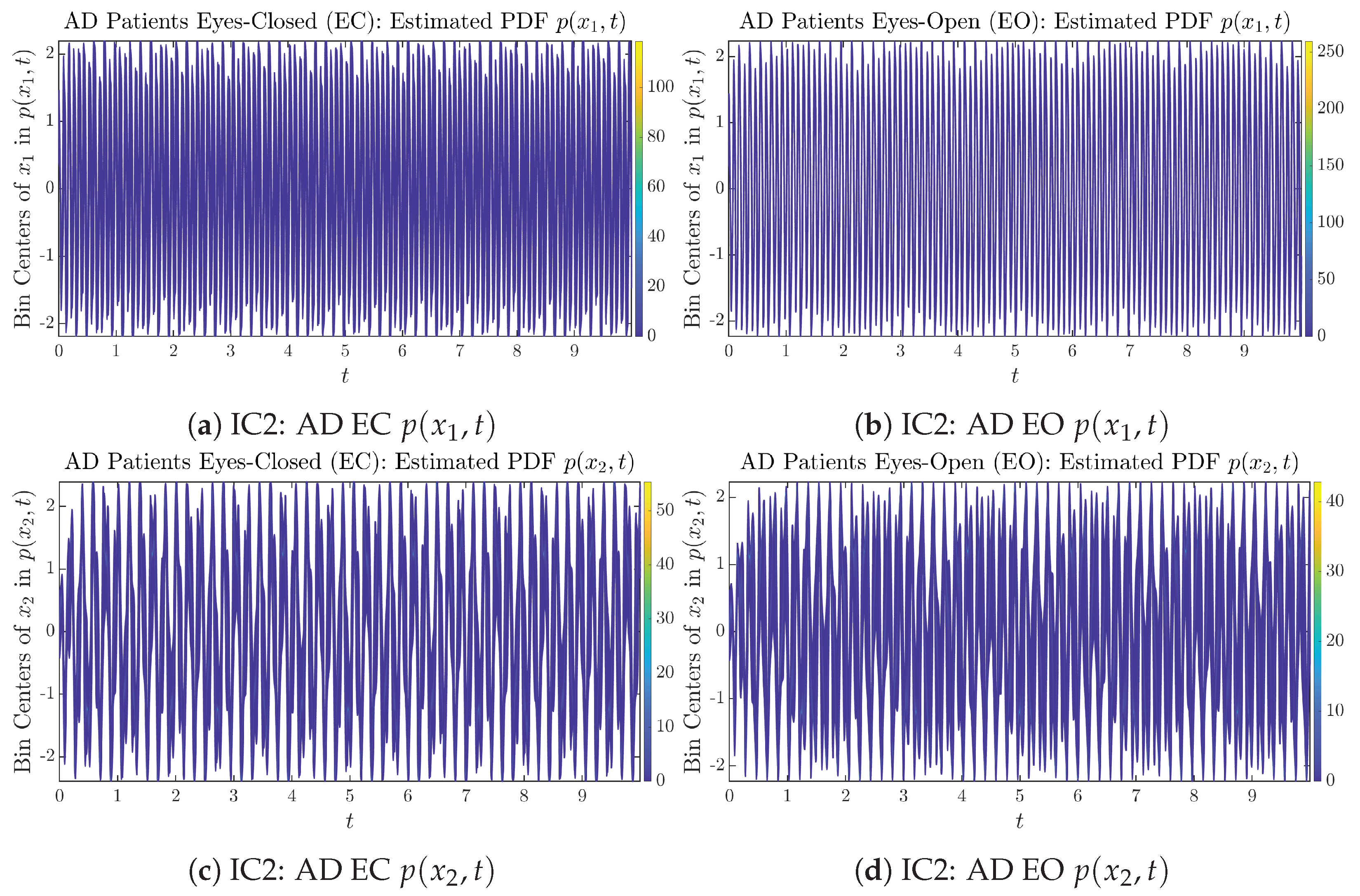
3.2. Time Evolution of PDF and
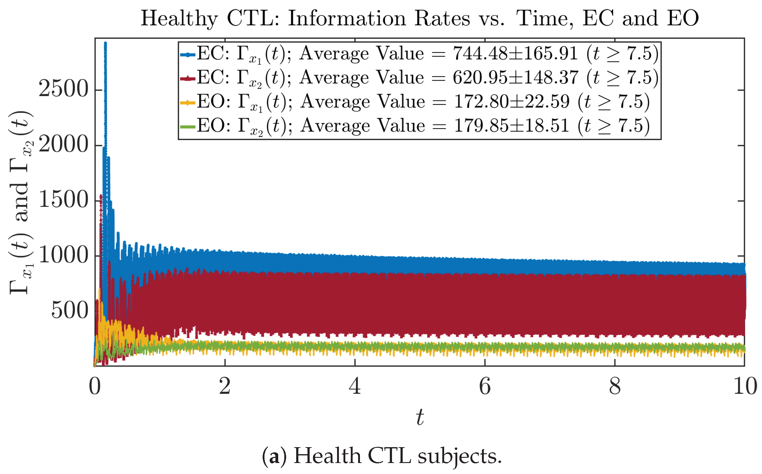
3.3. Information Rates and
3.3.1. Time Evolution
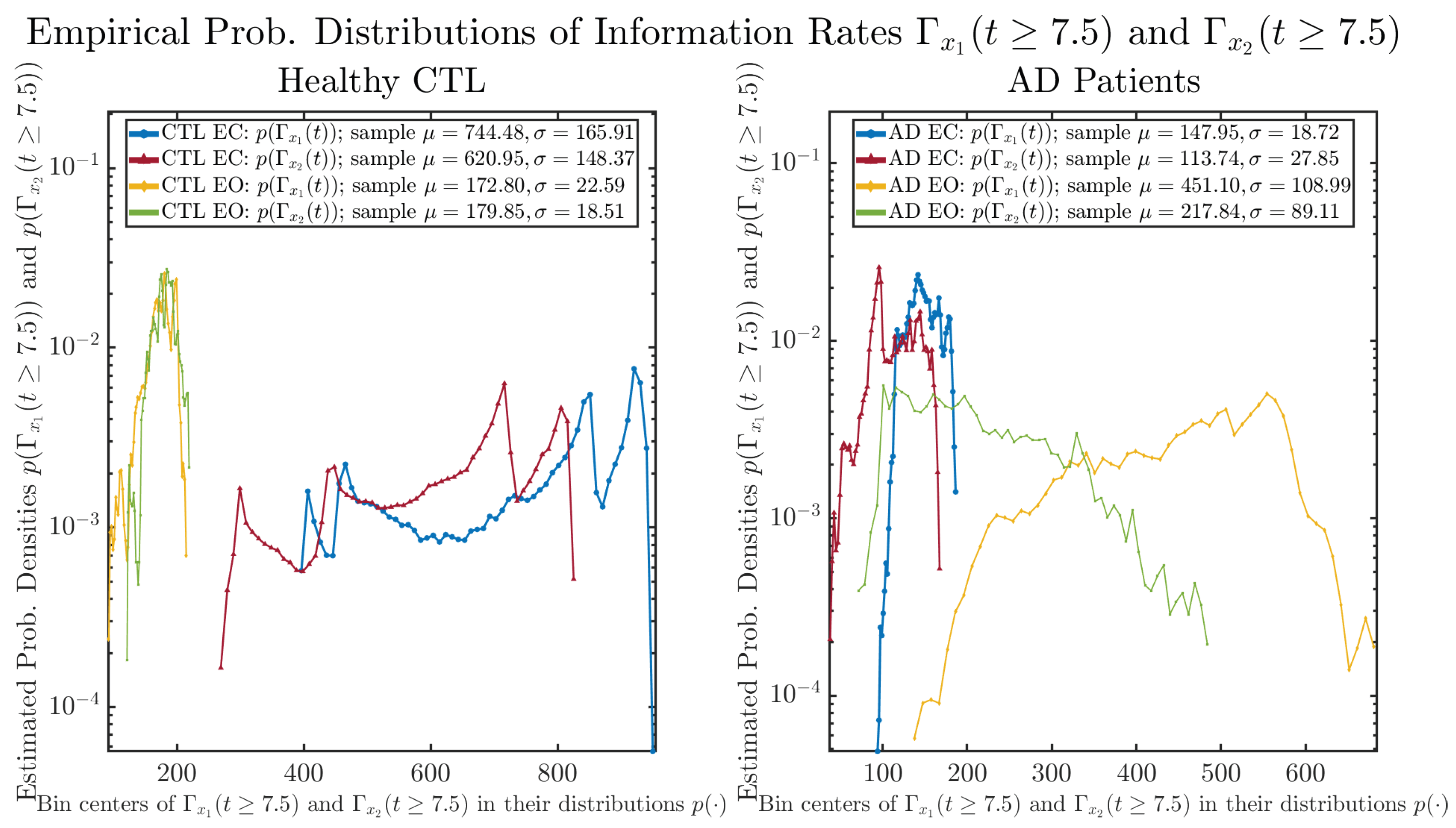
3.3.2. Empirical Probability Distribution (for )
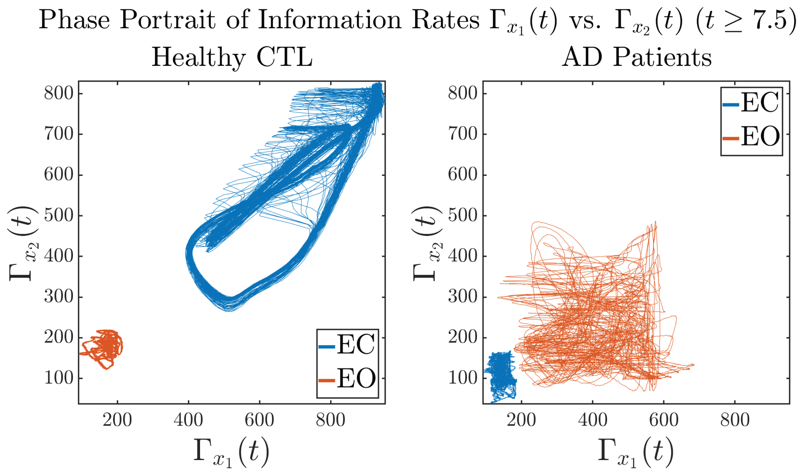
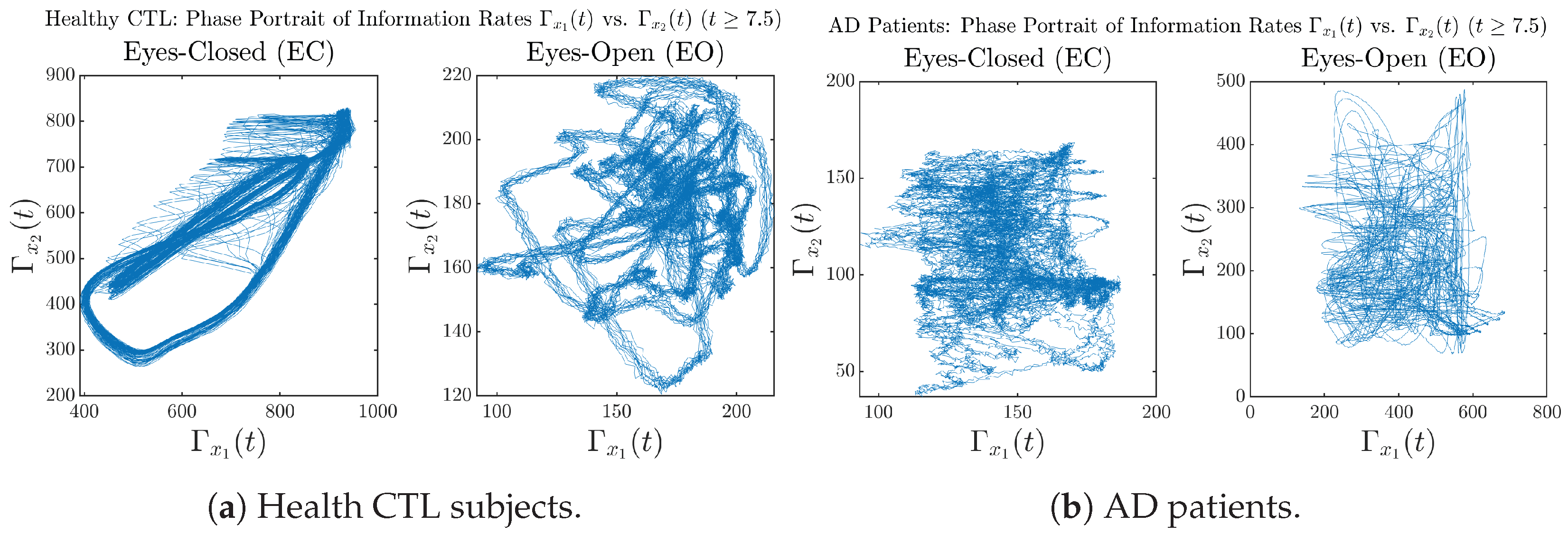
3.3.3. Phase Portraits (for )
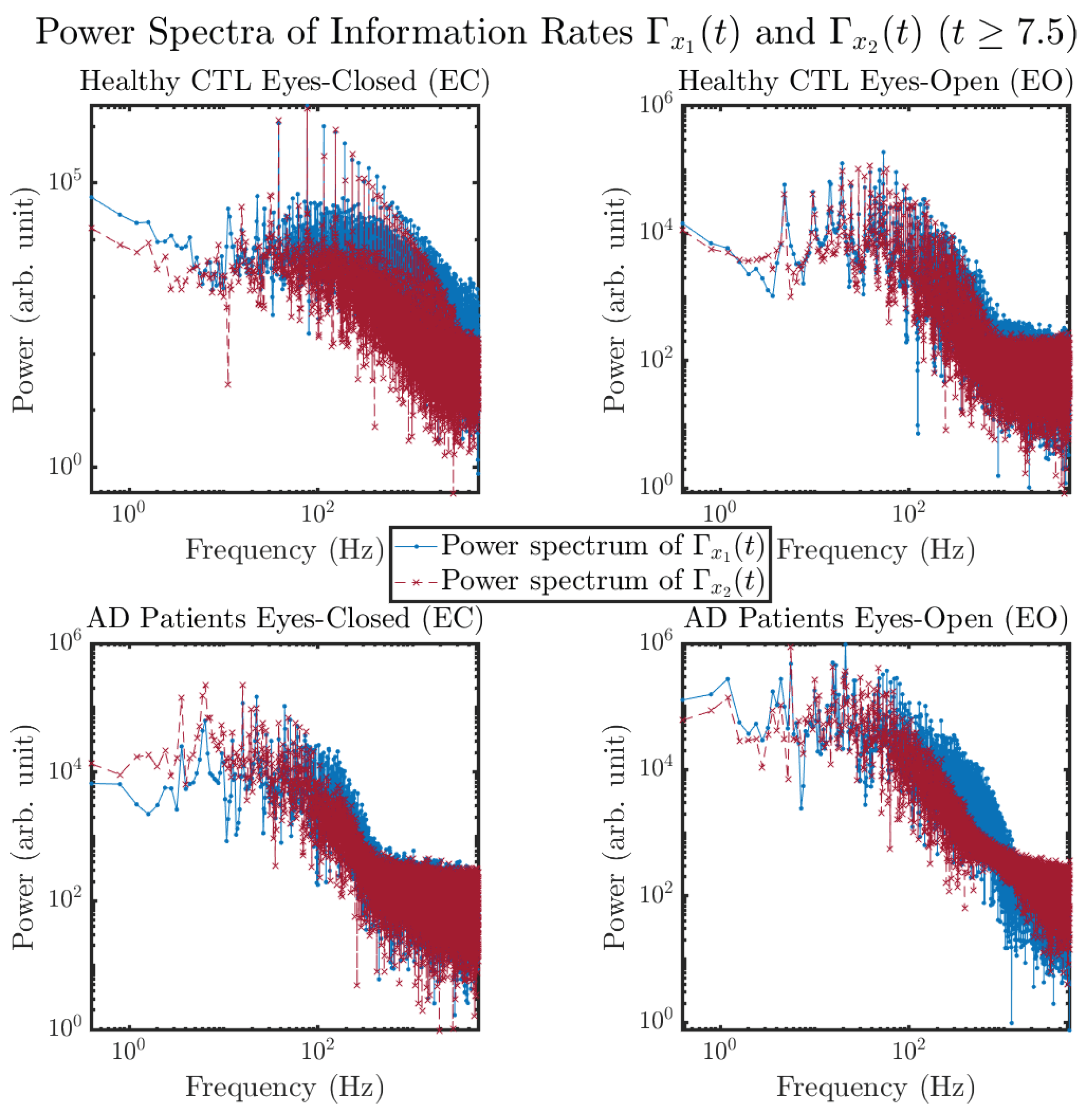
3.3.4. Power Spectra (for )
3.4. Causal Information Rates , and Net Causal Information Rates
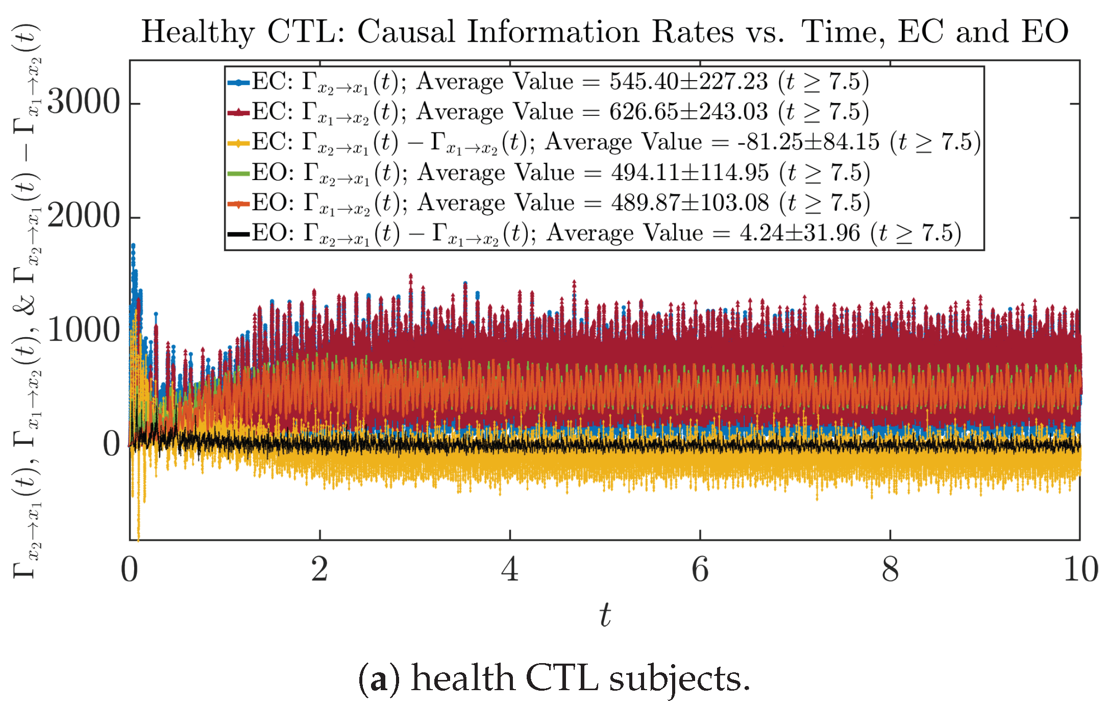
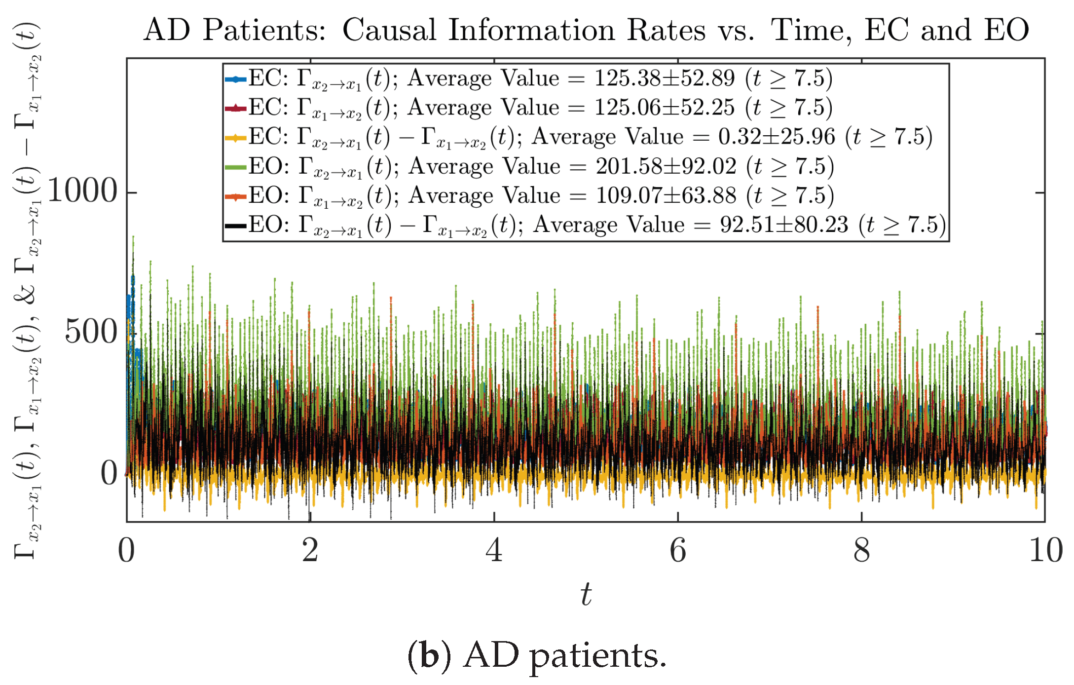
3.4.1. Time Evolution
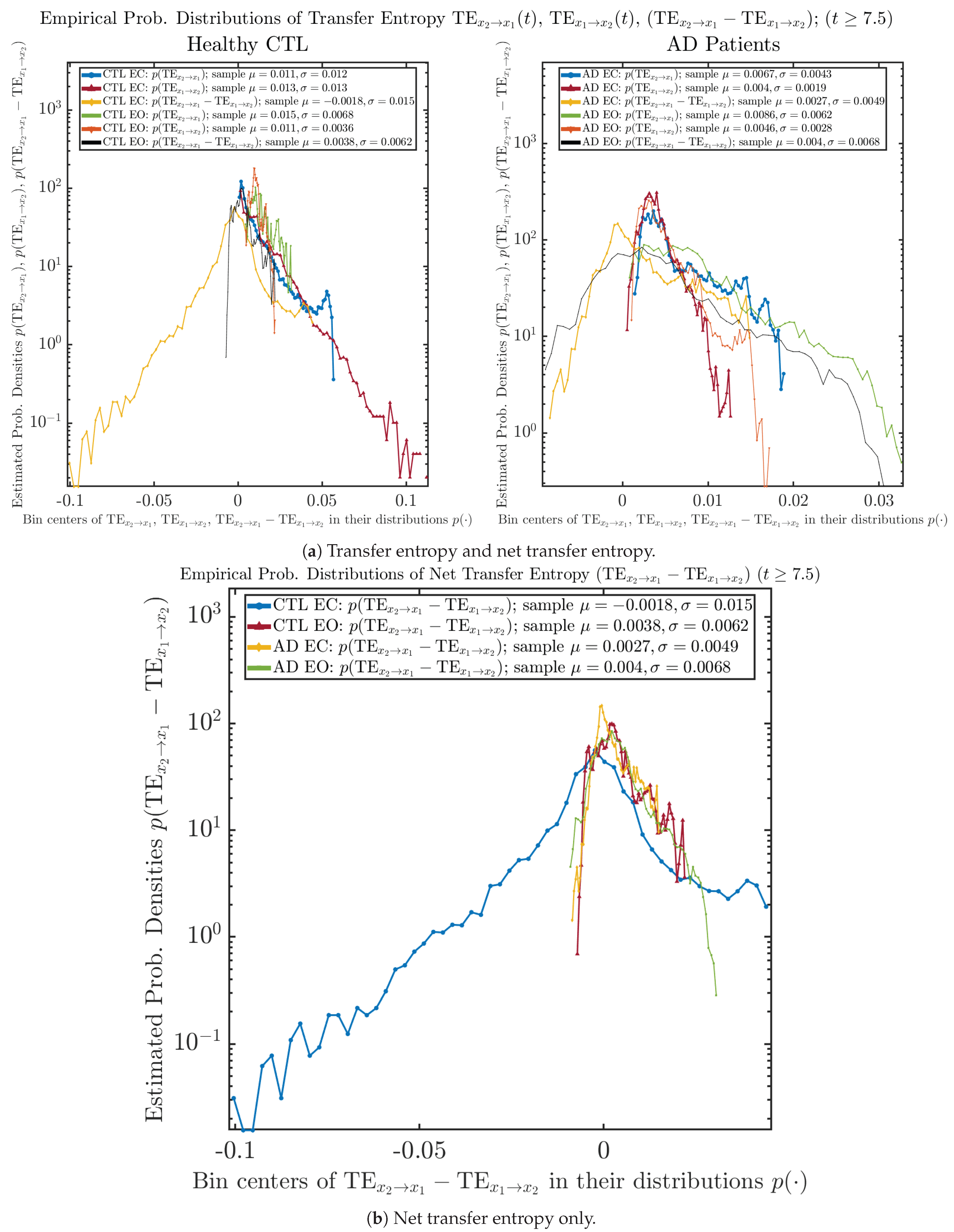
3.4.2. Empirical Probability Distribution (for )
4. Discussion
5. Conclusions
Author Contributions
Funding
Data Availability Statement
Acknowledgments
Conflicts of Interest
Abbreviations
| probability density function | |
| SDE | stochastic differential equation |
| IC | Initial Conditions (in terms of initial Gaussian distributions) |
| CTL | healthy control (subjects) |
| AD | Alzheimer’s disease |
| EC | eyes-closed |
| EO | eyes-open |
| TE | transfer entropy |
Appendix A. Finer Details of Numerical Estimation Techniques
- Using 2D trapezoidal rule for both and , that is, , and . In other words, when calculating , instead of estimating marginal PDF and directly by 1D histograms (using the relevant functions in MATLAB or Python), one first estimates the joint PDF and by 2D histograms and integrates over by trapezoidal summation on it. This will reduce the value of estimated , and integrals over both and are both estimated by trapezoidal summation.
- Using the 1D trapezoidal rule for both and , that is, , and . In this approach, the marginal PDF , where the equal sign holds exactly for the regular or naive summation . This is because the histogram estimation in MATLAB and Python is performed by counting the occurrence of data samples inside each bin, and the probability (mass) is estimated as , and the density is estimated as , where is the width of the x-th bin (and for 2D histogram, this is replaced by bin area ), and therefore, summing over is aggregating the 2D bins of and combining or mixing samples with -values/coordinates in the same -bin (but with -values/coordinates in different -bins) together. In other words, it is always true that , where is the number of samples inside the -th bin and is number of samples inside the -th bin in 2D, and hence, for estimated probability (mass), , and for estimated PDFs, , which is why holds exactly for numerically estimated marginal and joint PDFs using histograms, which is consistent with the theoretical relation between marginal and joint PDFs , and this has been numerically verified using the relevant 1D and 2D histogram functions in MATLAB and Python, i.e., by (naively) summing the estimated joint PDF over , and the (naively) summed marginal is exactly the same as the one estimated directly by 1D histogram function. So in this approach, integral over is estimated by naive summation on , but integral over is estimated by trapezoidal summation on .
Appendix B. Complete Results: All Six Groups of Initial Conditions
Appendix B.1. Sample Trajectories of and
Appendix B.1.1. Initial Conditions No.1 (IC1)


Appendix B.1.2. Initial Conditions No.2 (IC2)


Appendix B.1.3. Initial Conditions No.3 (IC3)


Appendix B.1.4. Initial Conditions No.4 (IC4)


Appendix B.1.5. Initial Conditions No.5 (IC5)


Appendix B.1.6. Initial Conditions No.6 (IC6)


Appendix B.2. Time Evolution of PDF and
Appendix B.2.1. Initial Conditions No.1 (IC1)


Appendix B.2.2. Initial Conditions No.2 (IC2)


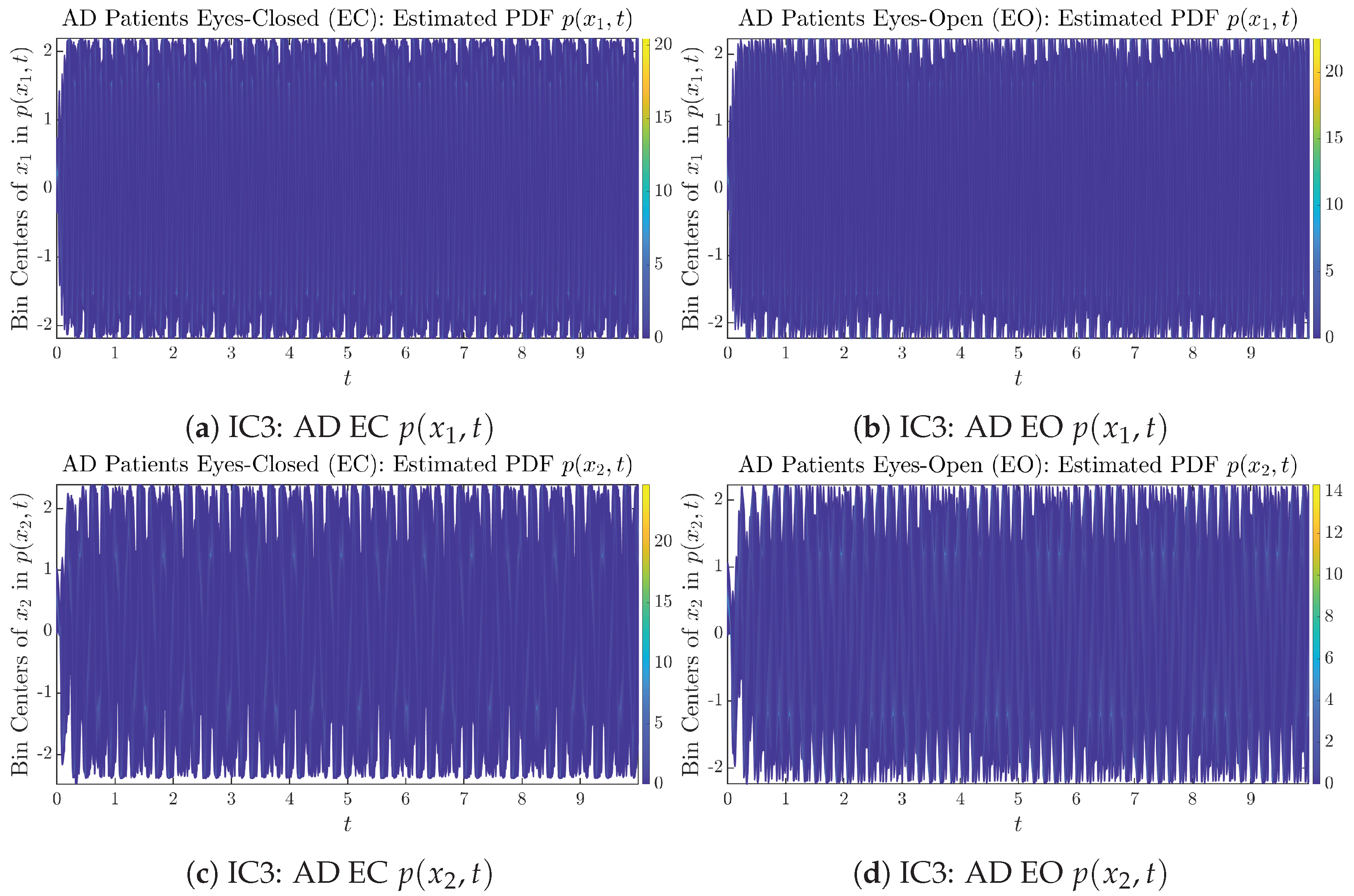
Appendix B.2.3. Initial Conditions No.3 (IC3)


Appendix B.2.4. Initial Conditions No.4 (IC4)


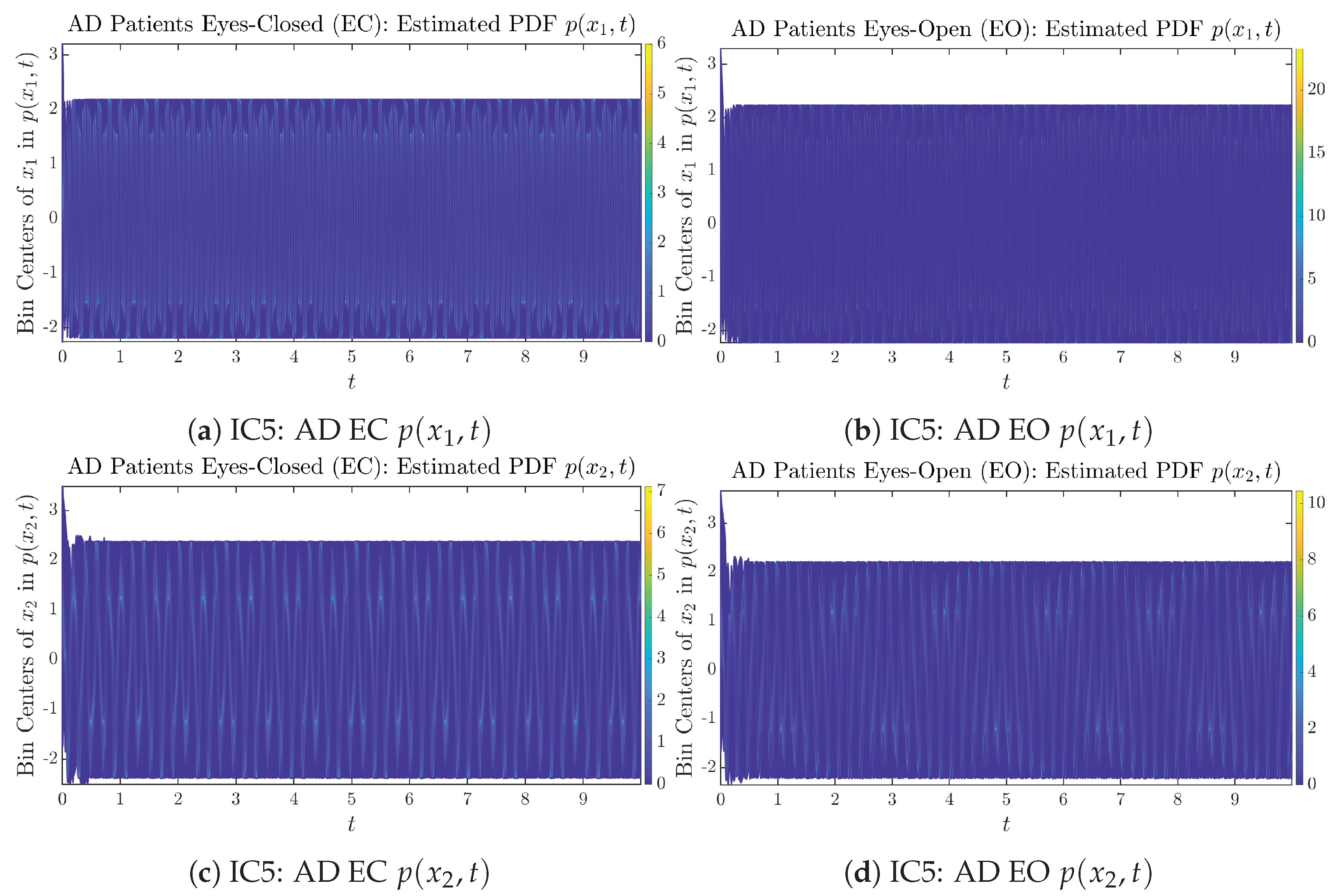
Appendix B.2.5. Initial Conditions No.5 (IC5)


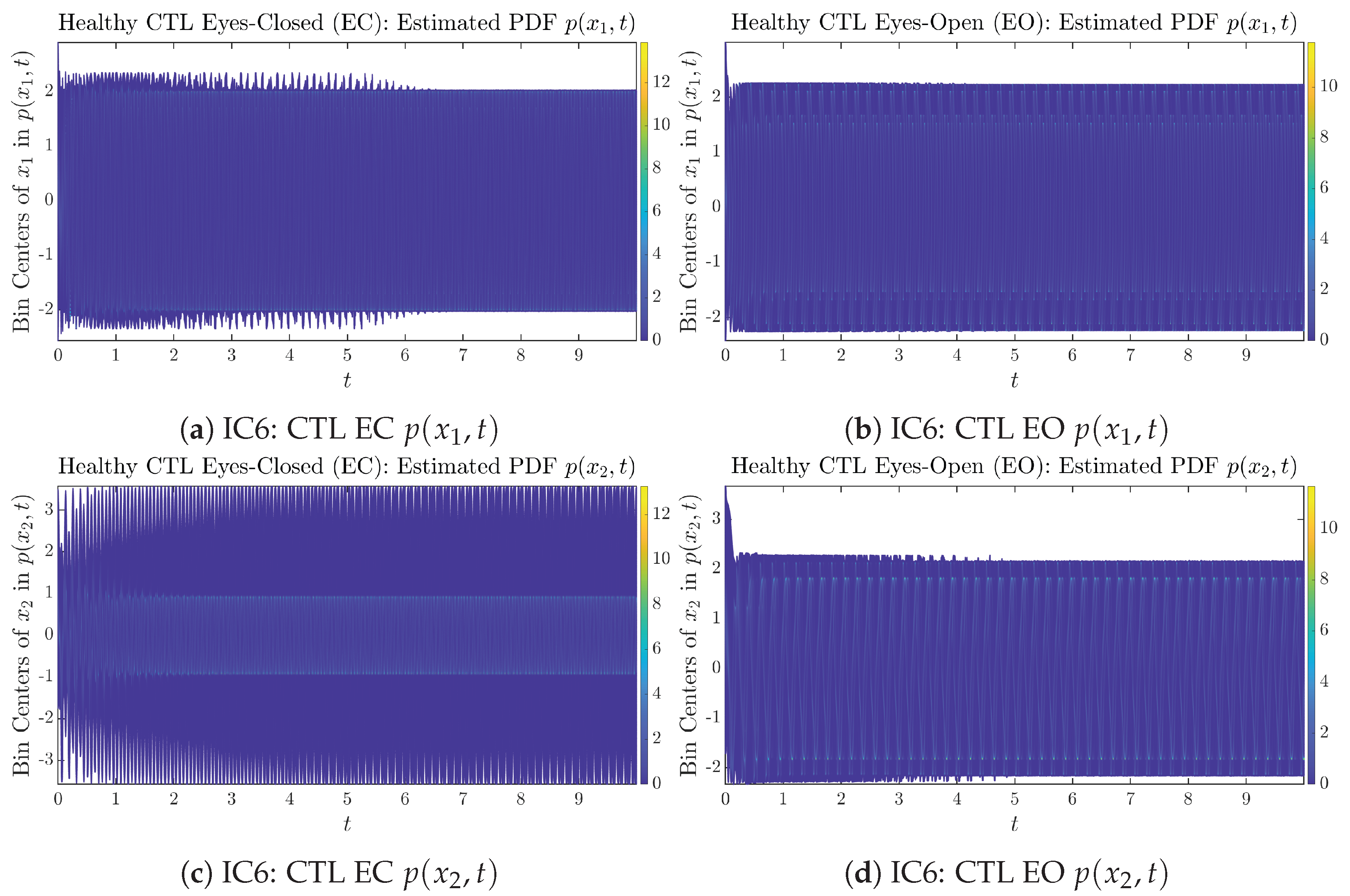
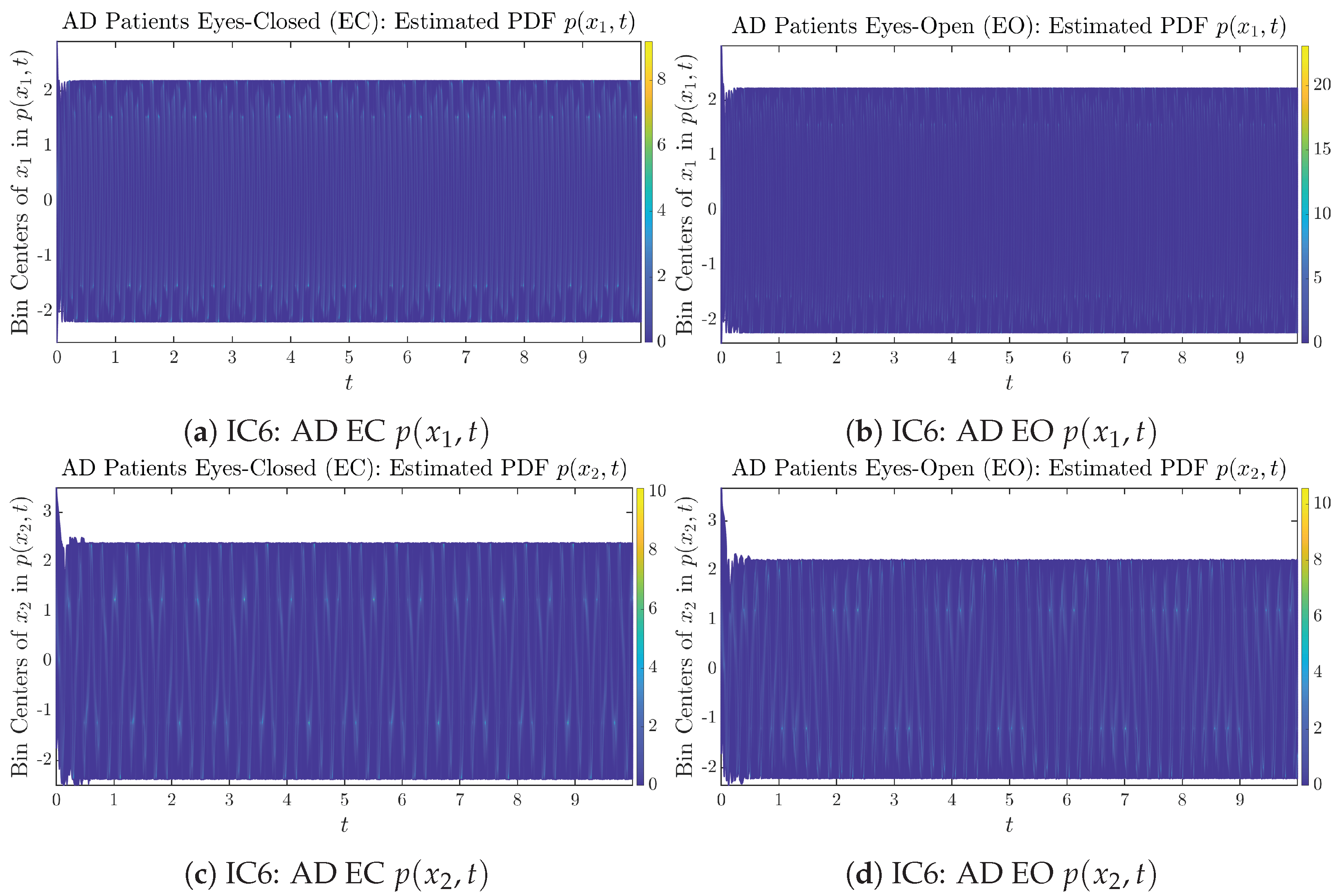
Appendix B.2.6. Initial Conditions No.6 (IC6)


Appendix B.3. Information Rates and
Appendix B.3.1. Time Evolution: Information Rates
Initial Conditions No.1 (IC1)

Initial Conditions No.2 (IC2)

Initial Conditions No.3 (IC3)

Initial Conditions No.4 (IC4)

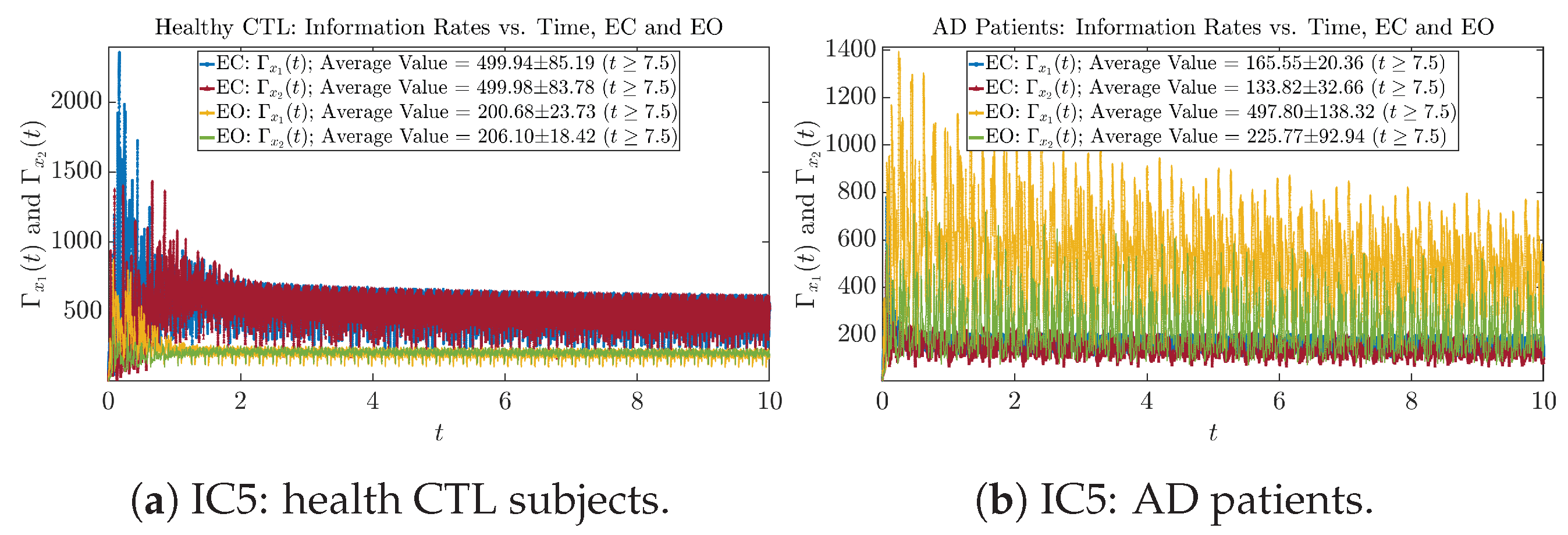
Initial Conditions No.5 (IC5)

Initial Conditions No.6 (IC6)

Appendix B.3.2. Empirical Probability Distribution: Information Rates (for )

Appendix B.3.3. Phase Portraits: Information Rates (for )

Initial Conditions No.1 (IC1):

Initial Conditions No.2 (IC2):

Initial Conditions No.3 (IC3):

Initial Conditions No.4 (IC4):

Initial Conditions No.5 (IC5):

Initial Conditions No.6 (IC6):

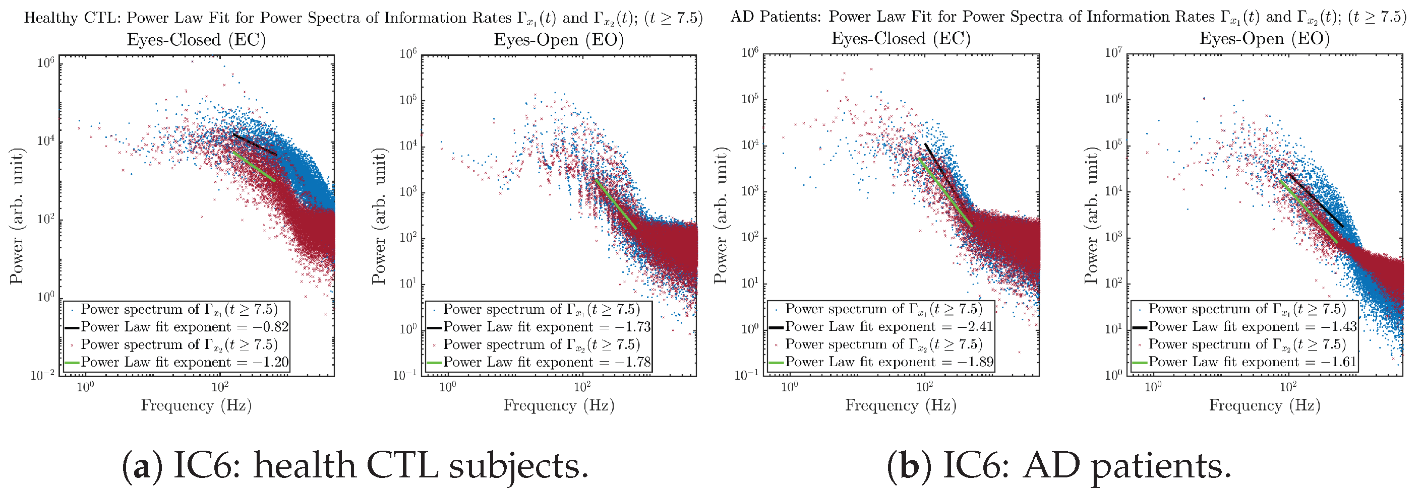
Appendix B.3.4. Power Spectra: Information Rates (for )
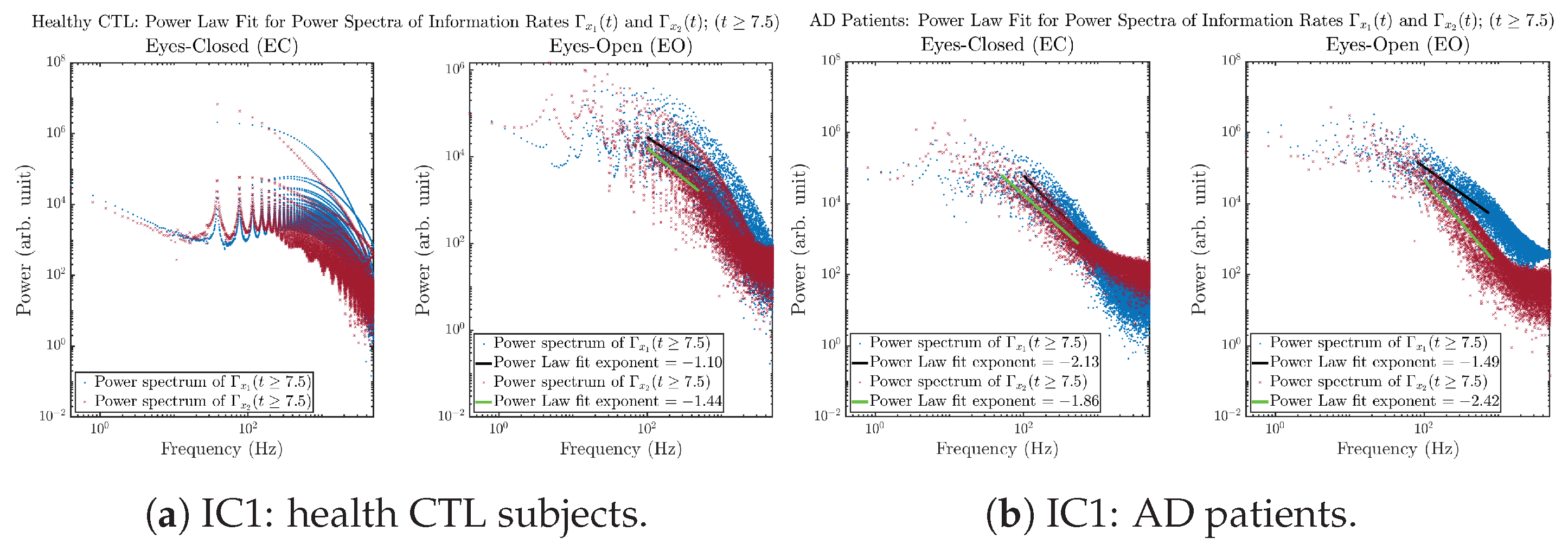
Initial Conditions No.1 (IC1):

Initial Conditions No.2 (IC2):

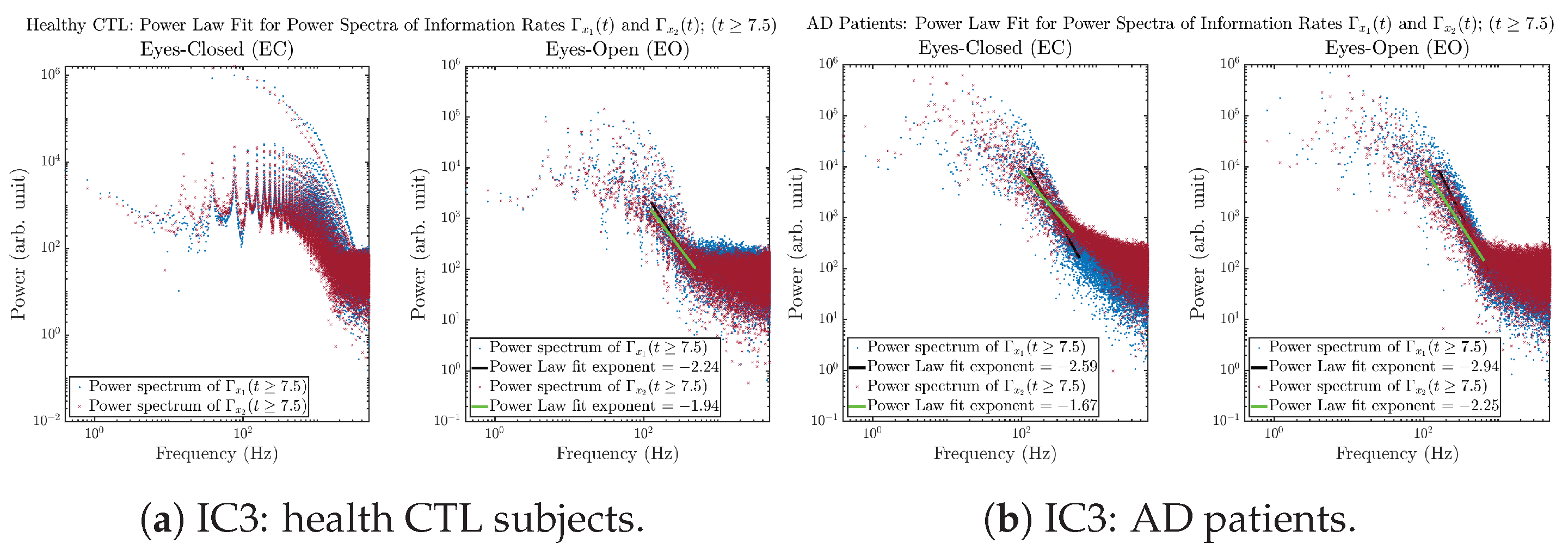
Initial Conditions No.3 (IC3):

Initial Conditions No.4 (IC4):

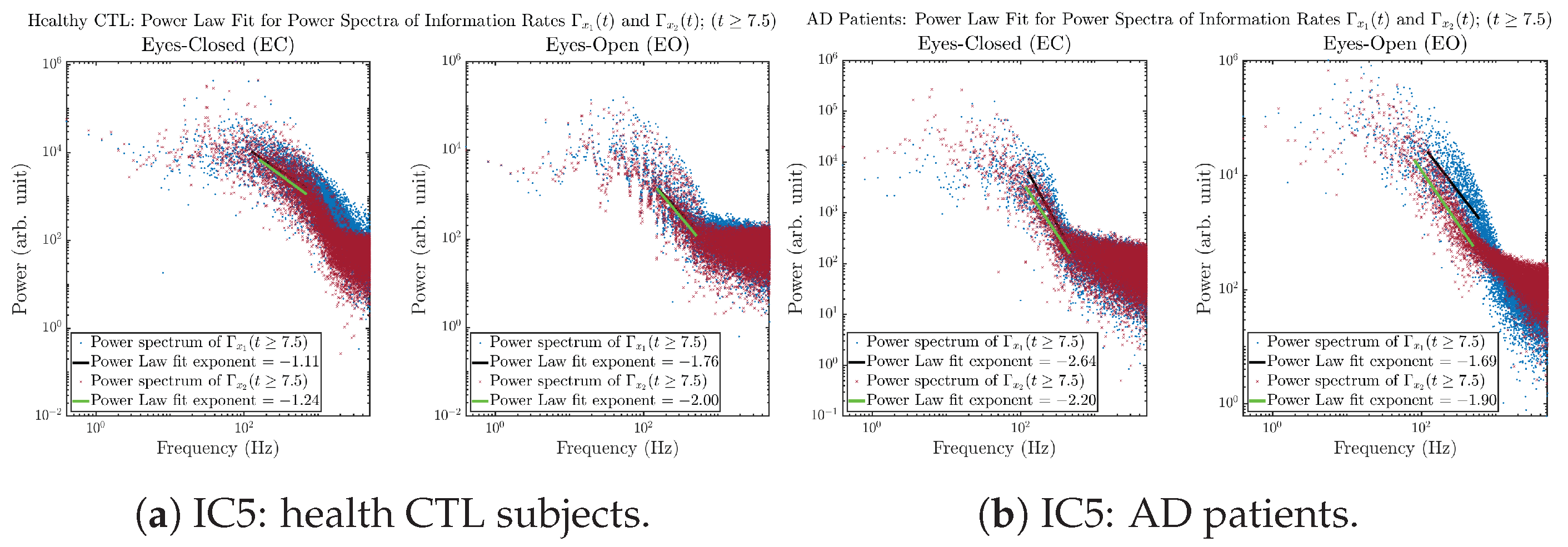
Initial Conditions No.5 (IC5):

Initial Conditions No.6 (IC6):

Appendix B.4. Shannon Differential Entropy of and
Appendix B.4.1. Time Evolution: Shannon Differential Entropy
Initial Conditions No.1 (IC1):

Initial Conditions No.2 (IC2):

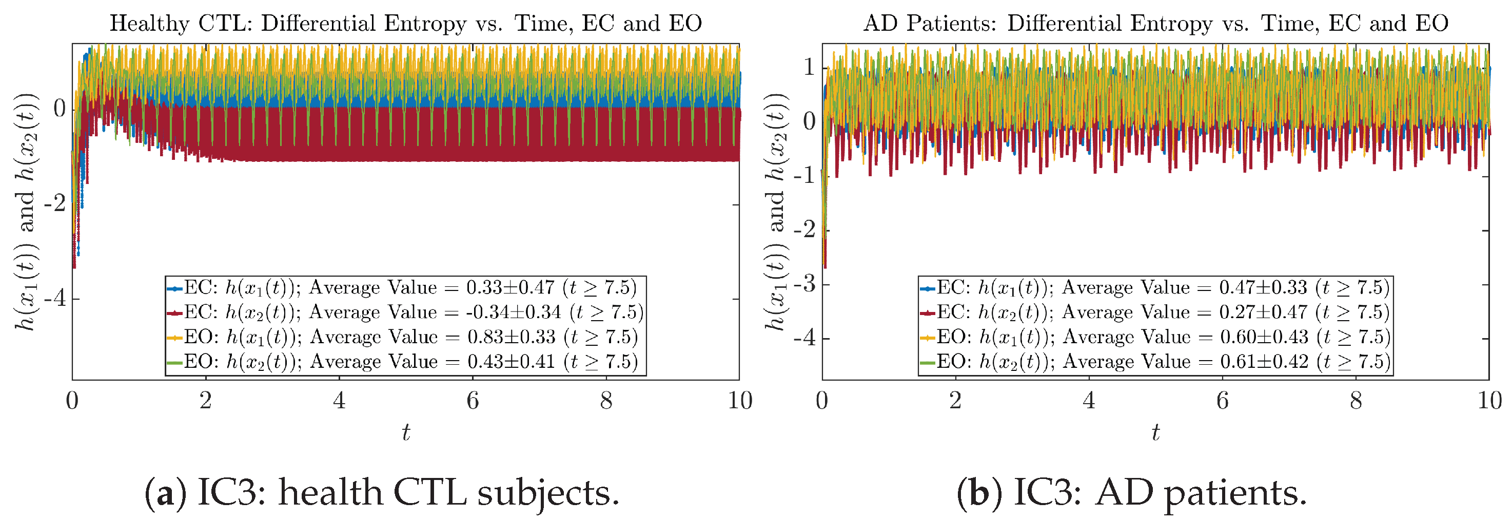
Initial Conditions No.3 (IC3):

Initial Conditions No.4 (IC4):

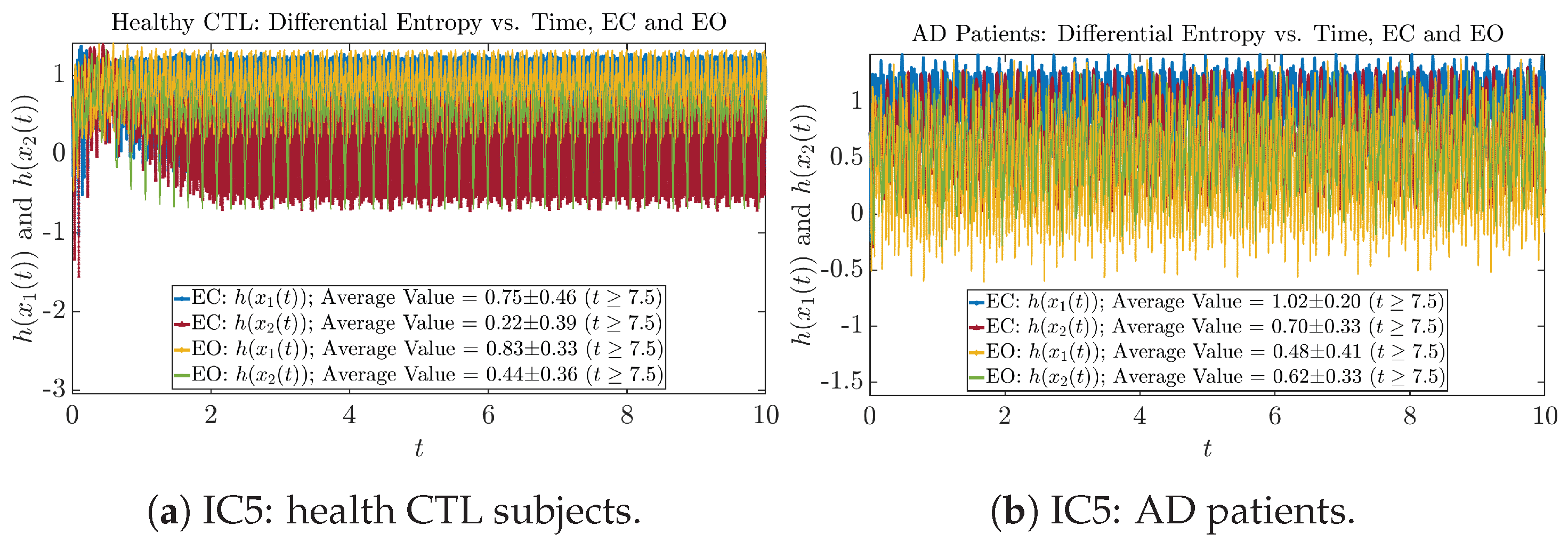
Initial Conditions No.5 (IC5):

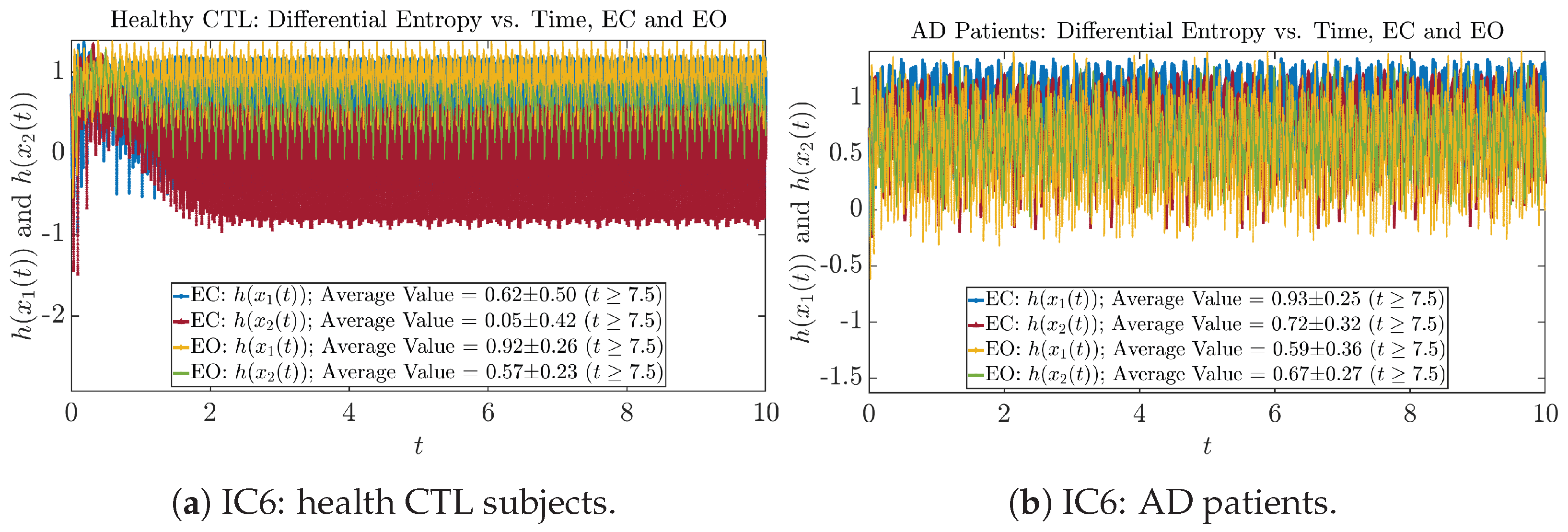
Initial Conditions No.6 (IC6):

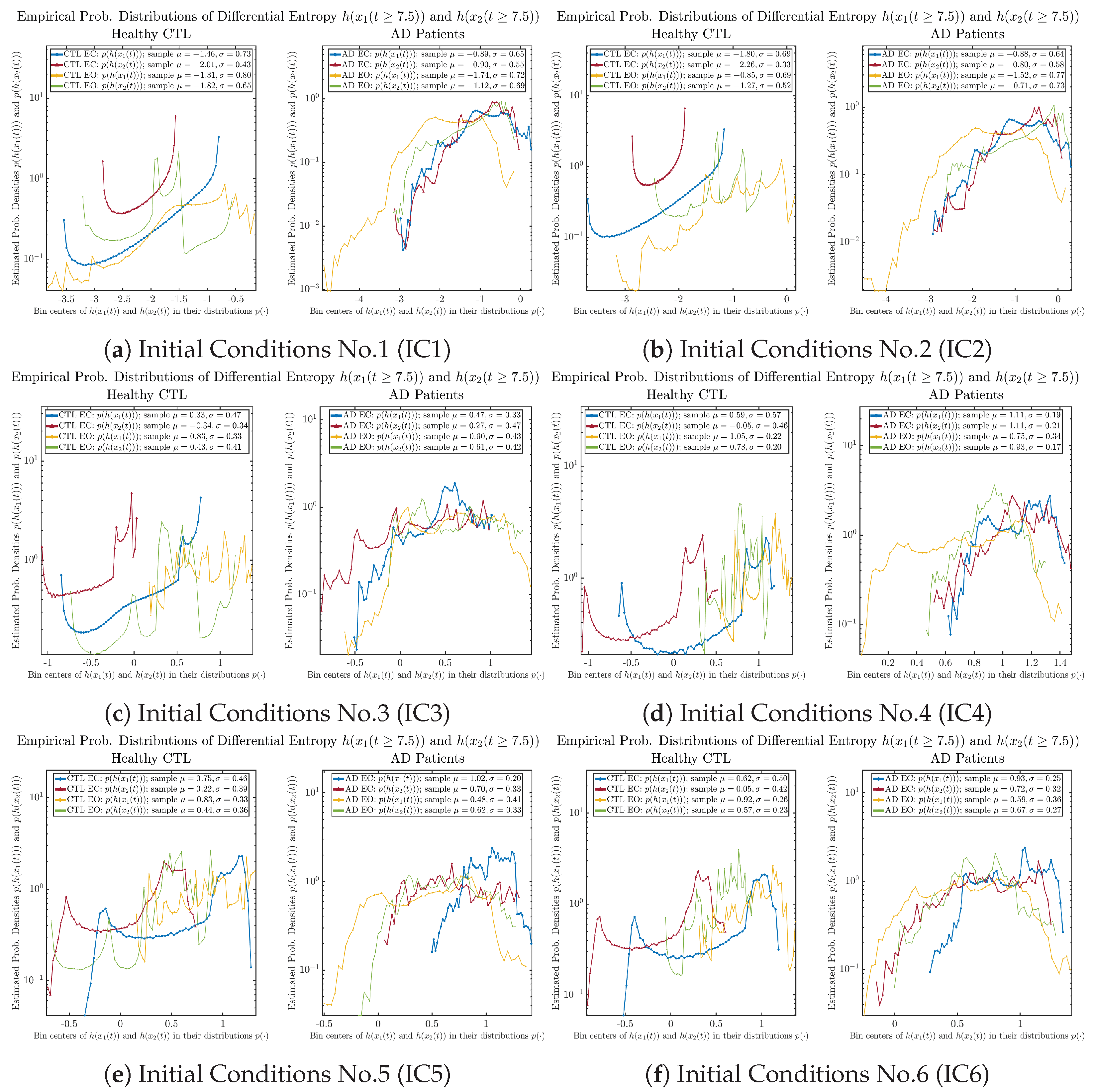
Appendix B.4.2. Empirical Probability Distribution: Shannon Differential Entropy (for )

Appendix B.4.3. Phase Portraits: Shannon Differential Entropy (for )

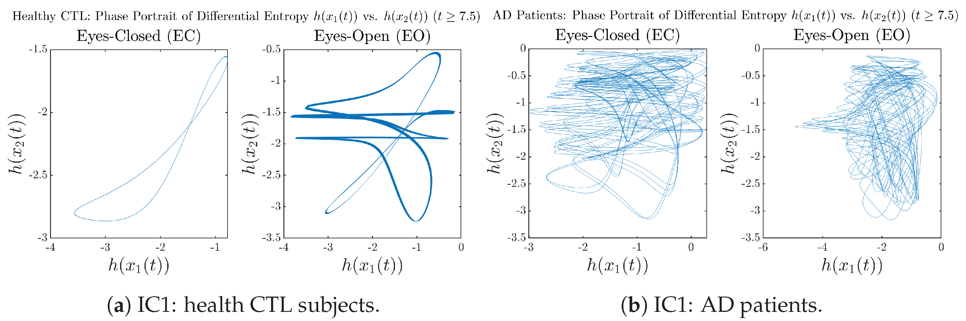
Initial Conditions No.1 (IC1):

Initial Conditions No.2 (IC2):

Initial Conditions No.3 (IC3):

Initial Conditions No.4 (IC4):

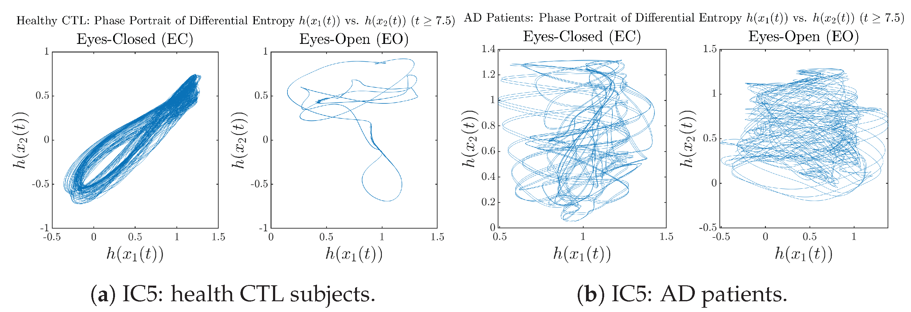
Initial Conditions No.5 (IC5):

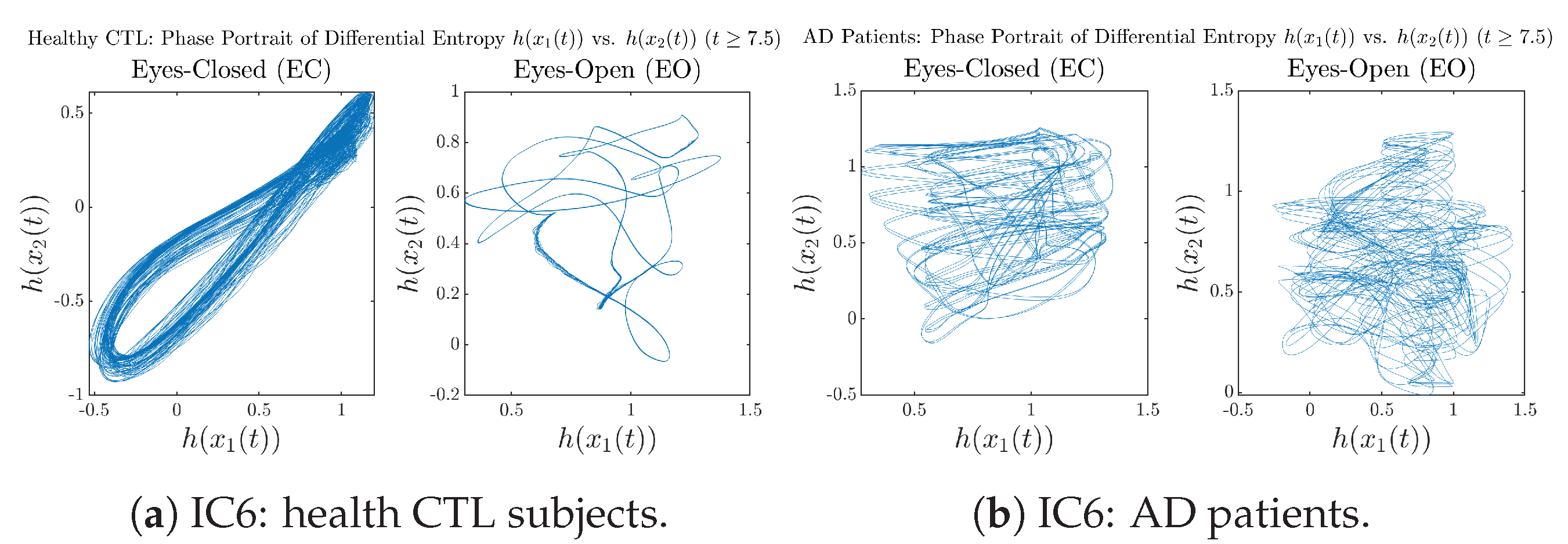
Initial Conditions No.6 (IC6):

Appendix B.4.4. Power Spectra: Shannon Differential Entropy (for )

Appendix B.5. Causal Information Rates , and Net Causal Information Rates
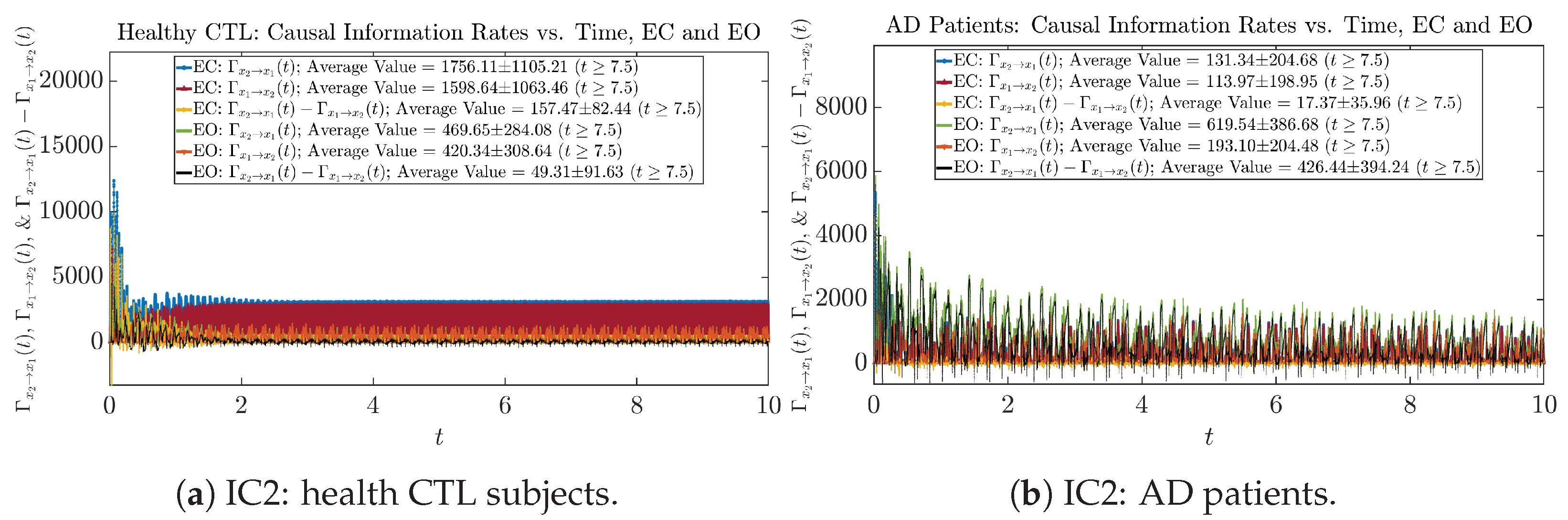
Appendix B.5.1. Time Evolution: Causal Information Rates
Initial Conditions No.1 (IC1):

Initial Conditions No.2 (IC2):

Initial Conditions No.3 (IC3):

Initial Conditions No.4 (IC4):

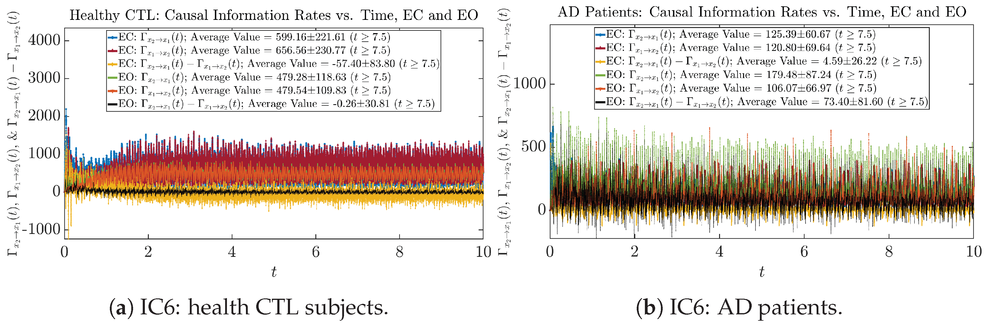
Initial Conditions No.5 (IC5):

Initial Conditions No.6 (IC6):

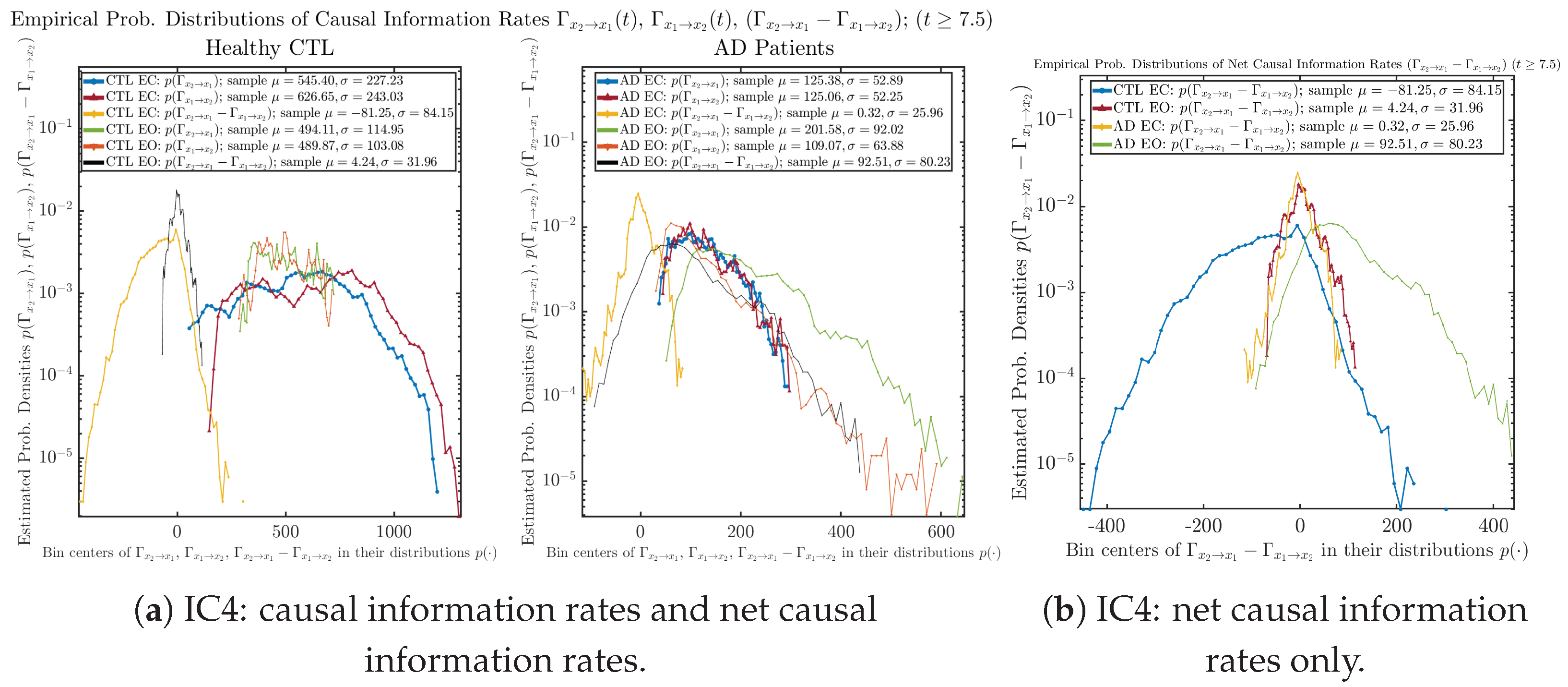
Appendix B.5.2. Empirical Probability Distribution: Causal Information Rates (for )
Initial Conditions No.1 (IC1):

Initial Conditions No.2 (IC2):

Initial Conditions No.3 (IC3):

Initial Conditions No.4 (IC4):

Initial Conditions No.5 (IC5):

Initial Conditions No.6 (IC6):

Appendix B.6. Causality Based on Transfer Entropy (TE)
Appendix B.6.1. Time Evolution: Transfer Entropy (TE)
Initial Conditions No.1 (IC1):

Initial Conditions No.2 (IC2):

Initial Conditions No.3 (IC3):

Initial Conditions No.4 (IC4):

Initial Conditions No.5 (IC5):

Initial Conditions No.6 (IC6):

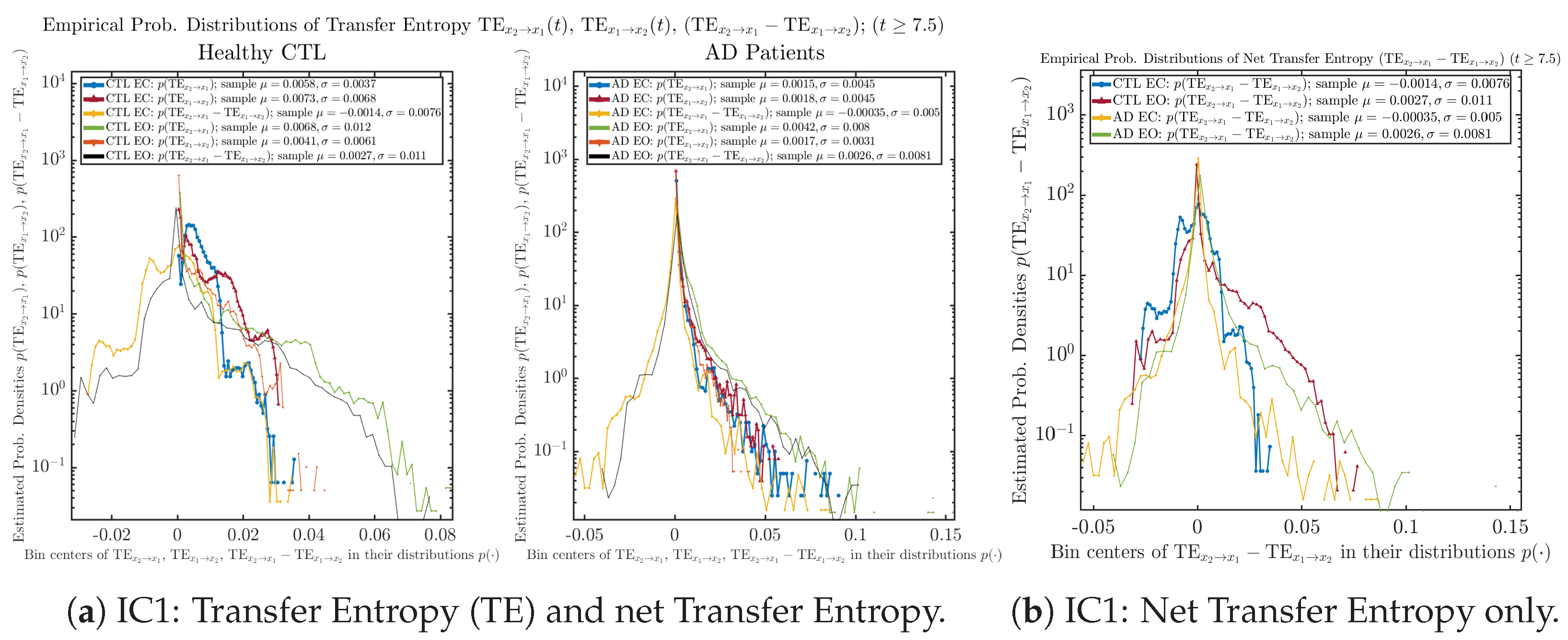
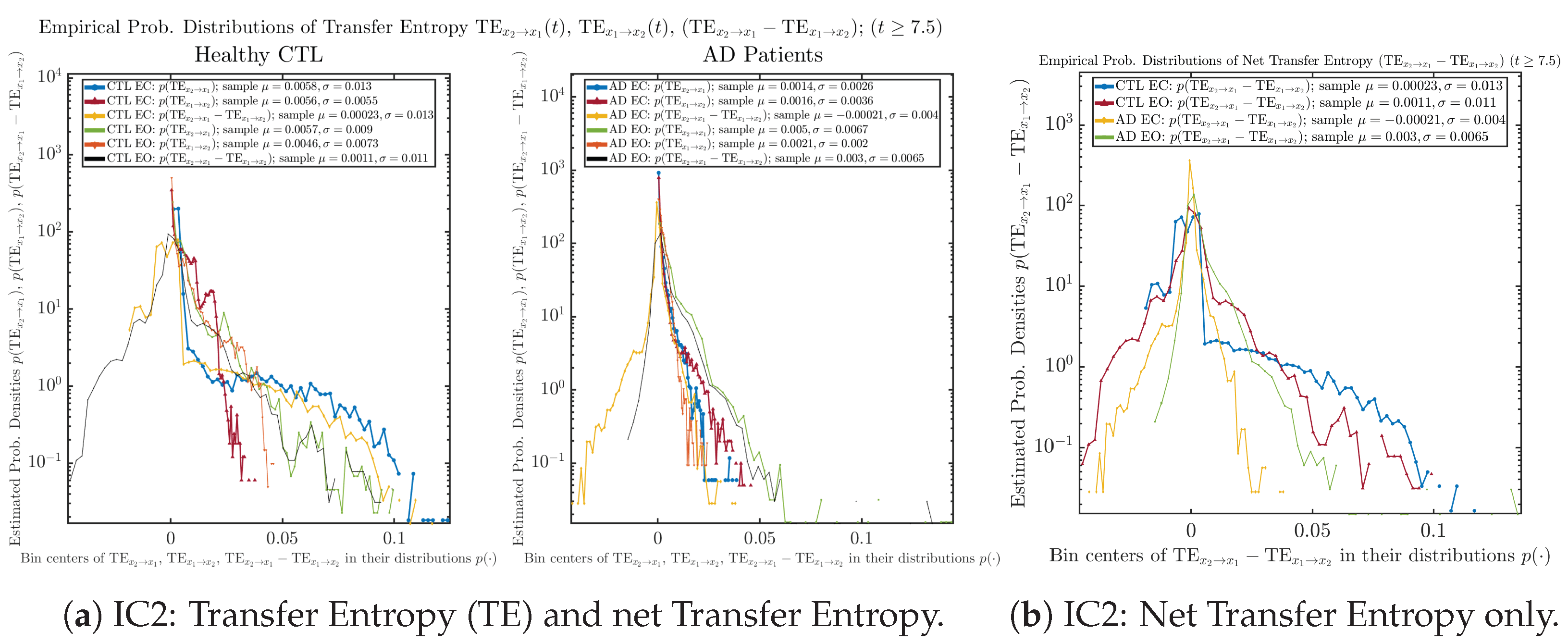
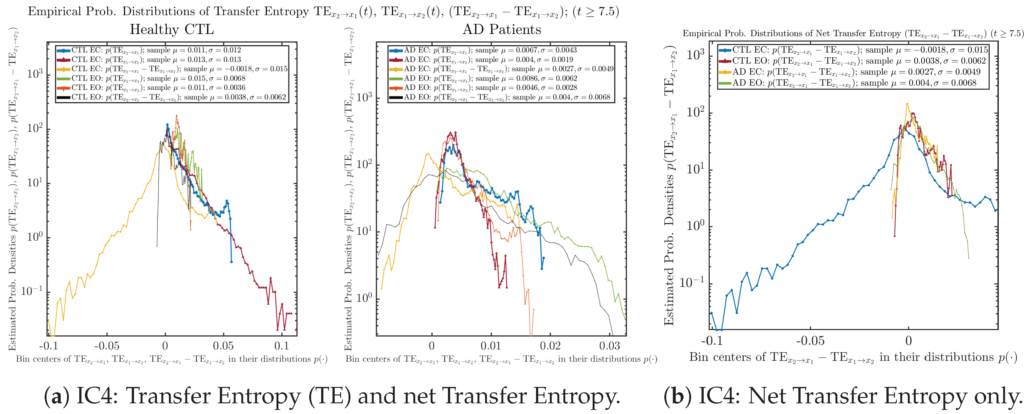
Appendix B.6.2. Empirical Probability Distribution: Transfer Entropy (TE) (for )
Initial Conditions No.1 (IC1):

Initial Conditions No.2 (IC2):

Initial Conditions No.3 (IC3):

Initial Conditions No.4 (IC4):

Initial Conditions No.5 (IC5):

Initial Conditions No.6 (IC6):

References
- Ghorbanian, P.; Ramakrishnan, S.; Ashrafiuon, H. Stochastic Non-Linear Oscillator Models of EEG: The Alzheimer’s Disease Case. Front. Comput. Neurosci. 2015, 9, 48. [Google Scholar] [CrossRef]
- Szuflitowska, B.; Orlowski, P. Statistical and Physiologically Analysis of Using a Duffing-van Der Pol Oscillator to Modeled Ictal Signals. In Proceedings of the 2020 16th International Conference on Control, Automation, Robotics and Vision (ICARCV), Shenzhen, China, 13–15 December 2020; pp. 1137–1142. [Google Scholar] [CrossRef]
- Nguyen, P.T.M.; Hayashi, Y.; Baptista, M.D.S.; Kondo, T. Collective Almost Synchronization-Based Model to Extract and Predict Features of EEG Signals. Sci. Rep. 2020, 10, 16342. [Google Scholar] [CrossRef] [PubMed]
- Guguloth, S.; Agarwal, V.; Parthasarathy, H.; Upreti, V. Synthesis of EEG Signals Modeled Using Non-Linear Oscillator Based on Speech Data with EKF. Biomed. Signal Process. Control 2022, 77, 103818. [Google Scholar] [CrossRef]
- Szuflitowska, B.; Orlowski, P. Analysis of Parameters Distribution of EEG Signals for Five Epileptic Seizure Phases Modeled by Duffing Van Der Pol Oscillator. In Proceedings of the Computational Science—ICCS 2022, London, UK, 21–23 June 2022; Groen, D., De Mulatier, C., Paszynski, M., Krzhizhanovskaya, V.V., Dongarra, J.J., Sloot, P.M.A., Eds.; Springer International Publishing: Cham, Switzerland, 2022; Volume 13352, pp. 188–201. [Google Scholar] [CrossRef]
- Barry, R.J.; De Blasio, F.M. EEG Differences between Eyes-Closed and Eyes-Open Resting Remain in Healthy Ageing. Biol. Psychol. 2017, 129, 293–304. [Google Scholar] [CrossRef] [PubMed]
- Jennings, J.L.; Peraza, L.R.; Baker, M.; Alter, K.; Taylor, J.P.; Bauer, R. Investigating the Power of Eyes Open Resting State EEG for Assisting in Dementia Diagnosis. Alzheimer’s Res. Ther. 2022, 14, 109. [Google Scholar] [CrossRef] [PubMed]
- Restrepo, J.F.; Mateos, D.M.; López, J.M.D. A Transfer Entropy-Based Methodology to Analyze Information Flow under Eyes-Open and Eyes-Closed Conditions with a Clinical Perspective. Biomed. Signal Process. Control 2023, 86, 105181. [Google Scholar] [CrossRef]
- Klepl, D.; He, F.; Wu, M.; Marco, M.D.; Blackburn, D.J.; Sarrigiannis, P.G. Characterising Alzheimer’s Disease with EEG-Based Energy Landscape Analysis. IEEE J. Biomed. Health Inform. 2022, 26, 992–1000. [Google Scholar] [CrossRef] [PubMed]
- Gunawardena, R.; Sarrigiannis, P.G.; Blackburn, D.J.; He, F. Kernel-Based Nonlinear Manifold Learning for EEG-based Functional Connectivity Analysis and Channel Selection with Application to Alzheimer’s Disease. Neuroscience 2023, 523, 140–156. [Google Scholar] [CrossRef] [PubMed]
- Barry, R.J.; Clarke, A.R.; Johnstone, S.J.; Magee, C.A.; Rushby, J.A. EEG Differences between Eyes-Closed and Eyes-Open Resting Conditions. Clin. Neurophysiol. 2007, 118, 2765–2773. [Google Scholar] [CrossRef]
- Barry, R.J.; Clarke, A.R.; Johnstone, S.J.; Brown, C.R. EEG Differences in Children between Eyes-Closed and Eyes-Open Resting Conditions. Clin. Neurophysiol. 2009, 120, 1806–1811. [Google Scholar] [CrossRef]
- Matsutomo, N.; Fukami, M.; Kobayashi, K.; Endo, Y.; Kuhara, S.; Yamamoto, T. Effects of Eyes-Closed Resting and Eyes-Open Conditions on Cerebral Blood Flow Measurement Using Arterial Spin Labeling Magnetic Resonance Imaging. Neurol. Clin. Neurosci. 2023, 11, 10–16. [Google Scholar] [CrossRef]
- Agcaoglu, O.; Wilson, T.W.; Wang, Y.P.; Stephen, J.; Calhoun, V.D. Resting State Connectivity Differences in Eyes Open versus Eyes Closed Conditions. Hum. Brain Mapp. 2019, 40, 2488–2498. [Google Scholar] [CrossRef] [PubMed]
- Han, J.; Zhou, L.; Wu, H.; Huang, Y.; Qiu, M.; Huang, L.; Lee, C.; Lane, T.J.; Qin, P. Eyes-Open and Eyes-Closed Resting State Network Connectivity Differences. Brain Sci. 2023, 13, 122. [Google Scholar] [CrossRef] [PubMed]
- Miraglia, F.; Vecchio, F.; Bramanti, P.; Rossini, P.M. EEG Characteristics in “Eyes-Open” versus “Eyes-Closed” Conditions: Small-world Network Architecture in Healthy Aging and Age-Related Brain Degeneration. Clin. Neurophysiol. 2016, 127, 1261–1268. [Google Scholar] [CrossRef] [PubMed]
- Wei, J.; Chen, T.; Li, C.; Liu, G.; Qiu, J.; Wei, D. Eyes-Open and Eyes-Closed Resting States with Opposite Brain Activity in Sensorimotor and Occipital Regions: Multidimensional Evidences from Machine Learning Perspective. Front. Hum. Neurosci. 2018, 12, 422. [Google Scholar] [CrossRef] [PubMed]
- Springer, B.A.; Marin, R.; Cyhan, T.; Roberts, H.; Gill, N.W. Normative Values for the Unipedal Stance Test with Eyes Open and Closed. J. Geriatr. Phys. Ther. 2007, 30, 8. [Google Scholar] [CrossRef] [PubMed]
- Marx, E.; Deutschländer, A.; Stephan, T.; Dieterich, M.; Wiesmann, M.; Brandt, T. Eyes Open and Eyes Closed as Rest Conditions: Impact on Brain Activation Patterns. NeuroImage 2004, 21, 1818–1824. [Google Scholar] [CrossRef] [PubMed]
- Zhang, D.; Liang, B.; Wu, X.; Wang, Z.; Xu, P.; Chang, S.; Liu, B.; Liu, M.; Huang, R. Directionality of Large-Scale Resting-State Brain Networks during Eyes Open and Eyes Closed Conditions. Front. Hum. Neurosci. 2015, 9, 81. [Google Scholar] [CrossRef]
- Xu, P.; Huang, R.; Wang, J.; Van Dam, N.T.; Xie, T.; Dong, Z.; Chen, C.; Gu, R.; Zang, Y.F.; He, Y.; et al. Different Topological Organization of Human Brain Functional Networks with Eyes Open versus Eyes Closed. NeuroImage 2014, 90, 246–255. [Google Scholar] [CrossRef]
- Jeong, J. EEG Dynamics in Patients with Alzheimer’s Disease. Clin. Neurophysiol. 2004, 115, 1490–1505. [Google Scholar] [CrossRef]
- Pritchard, W.S.; Duke, D.W.; Coburn, K.L. Altered EEG Dynamical Responsivity Associated with Normal Aging and Probable Alzheimer’s Disease. Dementia 1991, 2, 102–105. [Google Scholar] [CrossRef]
- Thiruthummal, A.A.; Kim, E.j. Monte Carlo Simulation of Stochastic Differential Equation to Study Information Geometry. Entropy 2022, 24, 1113. [Google Scholar] [CrossRef] [PubMed]
- Kim, E.j.; Guel-Cortez, A.J. Causal Information Rate. Entropy 2021, 23, 1087. [Google Scholar] [CrossRef] [PubMed]
- Choong, H.J.; Kim, E.j.; He, F. Causality Analysis with Information Geometry: A Comparison. Entropy 2023, 25, 806. [Google Scholar] [CrossRef] [PubMed]
- Baravalle, R.; Rosso, O.A.; Montani, F. Causal Shannon–Fisher Characterization of Motor/Imagery Movements in EEG. Entropy 2018, 20, 660. [Google Scholar] [CrossRef] [PubMed]
- Montani, F.; Baravalle, R.; Montangie, L.; Rosso, O.A. Causal Information Quantification of Prominent Dynamical Features of Biological Neurons. Philos. Trans. R. Soc. A Math. Phys. Eng. Sci. 2015, 373, 20150109. [Google Scholar] [CrossRef] [PubMed]
- Higham, D.J. An Algorithmic Introduction to Numerical Simulation of Stochastic Differential Equations. SIAM Rev. 2001, 43, 525–546. [Google Scholar] [CrossRef]
- Guel-Cortez, A.-J.; Kim, E.-j. Information Geometric Theory in the Prediction of Abrupt Changes in System Dynamics. Entropy 2021, 23, 694. [Google Scholar] [CrossRef] [PubMed]
- Amari, S.i.; Nagaoka, H. Methods of Information Geometry; American Mathematical Soc.: Providence, RI, USA, 2000; Volume 191. [Google Scholar]
- Frieden, B.R. Science from Fisher Information; Cambridge University Press: Cambridge, UK, 2004; Volume 974. [Google Scholar]
- Facchi, P.; Kulkarni, R.; Man’ko, V.I.; Marmo, G.; Sudarshan, E.C.G.; Ventriglia, F. Classical and Quantum Fisher Information in the Geometrical Formulation of Quantum Mechanics. Phys. Lett. A 2010, 374, 4801–4803. [Google Scholar] [CrossRef]
- Itoh, M.; Shishido, Y. Fisher Information Metric and Poisson Kernels. Differ. Geom. Its Appl. 2008, 26, 347–356. [Google Scholar] [CrossRef]
- Sahann, R.; Möller, T.; Schmidt, J. Histogram Binning Revisited with a Focus on Human Perception. arXiv 2021, arXiv:cs/2109.06612. [Google Scholar] [CrossRef]
- Terrell, G.R.; Scott, D.W. Oversmoothed Nonparametric Density Estimates. J. Am. Stat. Assoc. 1985, 80, 209–214. [Google Scholar] [CrossRef]
- Budišić, M.; Mohr, R.M.; Mezić, I. Applied Koopmanism. Chaos Interdiscip. J. Nonlinear Sci. 2012, 22, 047510. [Google Scholar] [CrossRef] [PubMed]
- Koopman, B.O. Hamiltonian Systems and Transformation in Hilbert Space. Proc. Natl. Acad. Sci. USA 1931, 17, 315–318. [Google Scholar] [CrossRef]


| Parameter | Eyes-Closed (EC) | Eyes-Open (EO) |
|---|---|---|
| 7286.5 | 2427.2 | |
| 4523.5 | 499.92 | |
| 232.05 | 95.61 | |
| 10.78 | 103.36 | |
| 33.60 | 48.89 | |
| 0.97 | 28.75 | |
| 2.34 | 1.82 |
| Parameter | Eyes-Closed (EC) | Eyes-Open (EO) |
|---|---|---|
| 1742.1 | 3139.9 | |
| 1270.8 | 650.32 | |
| 771.99 | 101.1 | |
| 1.91 | 81.3 | |
| 63.7 | 56.3 | |
| 20.7 | 19.12 | |
| 1.78 | 1.74 |
| IC No.1 | IC No.2 | IC No.3 | IC No.4 | IC No.5 | IC No.6 | |
|---|---|---|---|---|---|---|
| 1.0 | 0.9 | 0.2 | 0.1 | 0.5 | 0.2 | |
| 0.5 | 0.1 | 0.5 | 0.5 | 0.9 | 0.9 | |
| 0 | 1.0 | 0.5 | 0.2 | 1.0 | 0.1 | |
| 0 | 0.5 | 1.0 | 1.0 | 0.8 | 0.5 | |
| 0.1 | 0.1 | 0.1 | 0.5 | 0.5 | 0.5 | |
| Num. of trajectories | ||||||
| Num. of time-steps | ||||||
| Total range of t |
| CTL EC | CTL EO | AD EC | AD EO | |
|---|---|---|---|---|
| 744.48 ± 165.91 | 172.80 ± 22.59 | 147.95 ± 18.72 | 451.10 ± 108.99 | |
| 620.95 ± 148.37 | 179.85 ± 18.51 | 113.74 ± 27.85 | 217.84 ± 89.11 | |
| 0.59 ± 0.57 | 1.05 ± 0.22 | 1.11 ± 0.19 | 0.73 ± 0.34 | |
| −0.05 ± 0.46 | 0.78 ± 0.20 | 1.11 ± 0.21 | 0.93 ± 0.17 |
| CTL EC | CTL EO | AD EC | AD EO | |
|---|---|---|---|---|
| 545.40 ± 227.23 | 494.11 ± 114.95 | 125.38 ± 52.89 | 201.58 ± 92.02 | |
| 626.65 ± 243.03 | 489.87 ± 103.08 | 125.06 ± 52.25 | 109.07 ± 63.88 | |
| −81.25 ± 84.15 | 4.24 ± 31.96 | 0.32 ± 25.96 | 92.51 ± 80.23 | |
| 0.011 ± 0.012 | 0.015 ± 0.0068 | 0.0067 ± 0.0043 | 0.0086 ± 0.0062 | |
| 0.013 ± 0.013 | 0.011 ± 0.0036 | 0.004 ± 0.0019 | 0.0046 ± 0.0028 | |
| −0.0018 ± 0.015 | 0.0038 ± 0.0062 | 0.0027 ± 0.0049 | 0.004 ± 0.0068 |
Disclaimer/Publisher’s Note: The statements, opinions and data contained in all publications are solely those of the individual author(s) and contributor(s) and not of MDPI and/or the editor(s). MDPI and/or the editor(s) disclaim responsibility for any injury to people or property resulting from any ideas, methods, instructions or products referred to in the content. |
© 2024 by the authors. Licensee MDPI, Basel, Switzerland. This article is an open access article distributed under the terms and conditions of the Creative Commons Attribution (CC BY) license (https://creativecommons.org/licenses/by/4.0/).
Share and Cite
Hua, J.-C.; Kim, E.-j.; He, F. Information Geometry Theoretic Measures for Characterizing Neural Information Processing from Simulated EEG Signals. Entropy 2024, 26, 213. https://doi.org/10.3390/e26030213
Hua J-C, Kim E-j, He F. Information Geometry Theoretic Measures for Characterizing Neural Information Processing from Simulated EEG Signals. Entropy. 2024; 26(3):213. https://doi.org/10.3390/e26030213
Chicago/Turabian StyleHua, Jia-Chen, Eun-jin Kim, and Fei He. 2024. "Information Geometry Theoretic Measures for Characterizing Neural Information Processing from Simulated EEG Signals" Entropy 26, no. 3: 213. https://doi.org/10.3390/e26030213
APA StyleHua, J.-C., Kim, E.-j., & He, F. (2024). Information Geometry Theoretic Measures for Characterizing Neural Information Processing from Simulated EEG Signals. Entropy, 26(3), 213. https://doi.org/10.3390/e26030213