A Novel Fault Diagnosis Method for a Power Transformer Based on Multi-Scale Approximate Entropy and Optimized Convolutional Networks

Abstract

Dissolved gas analysis (DGA) in transformer oil, which analyzes its gas content, is valuable for promptly detecting potential faults in oil-immersed transformers. Given the limitations of traditional transformer fault diagnostic methods, such as insufficient gas characteristic components and a high misjudgment rate for transformer faults, this study proposes a transformer fault diagnosis model based on multi-scale approximate entropy and optimized convolutional neural networks (CNNs). This study introduces an improved sparrow search algorithm (ISSA) for optimizing CNN parameters, establishing the ISSA-CNN transformer fault diagnosis model. The dissolved gas components in the transformer oil are analyzed, and the multi-scale approximate entropy of the gas content under different fault modes is calculated. The computed entropy values are then used as feature parameters for the ISSA-CNN model to derive diagnostic results. Experimental data analysis demonstrates that multi-scale approximate entropy effectively characterizes the dissolved gas components in the transformer oil, significantly improving the diagnostic efficiency. Comparative analysis with BPNN, ELM, and CNNs validates the effectiveness and superiority of the proposed ISSA-CNN diagnostic model across various evaluation metrics.

1. Introduction

Oil-immersed power transformers are vital components in power systems, primarily utilized for voltage regulation and the transmission and distribution of electrical energy [1]. These transformers utilize insulating oil for effective heat control. The design and operation of transformers directly impact the quality of the electrical energy and the reliability of the power system. Therefore, understanding the operational status of oil-immersed transformers and ensuring their safe and stable operation are crucial for the reliability of the power system [2].

The fault diagnosis method for oil-immersed transformers based on dissolved gas analysis (DGA) in oil has gained widespread application in recent years [3,4]. By analyzing the gas content in the transformer oil, this method can effectively identify the types of electrical faults, discover potential issues, and provide crucial information for proactive maintenance of transformers. As a result, it has become increasingly prevalent in the field. Currently, the traditional diagnostic methods for dissolved gases in transformer oil include the three-ratio method [5] and the Duval Triangle method [6]. However, these approaches suffer from shortcomings such as insufficient coding and excessive absoluteness, leading to a higher rate of misjudgment. This phenomenon results in their inability to accurately diagnose certain faults. Therefore, there are now various intelligent diagnostic methods for oil-immersed transformer faults based on DGA. These methods mainly include Artificial Neural Networks (ANNs), Support Vector Machines (SVMs), Expert Systems (ESs), Extreme Learning Machines (ELMs), etc. ANNs offer advantages, such as distributed parallel processing, adaptability, self-learning, associative memory, and non-linear mapping. Zhou et al. [7] proposed a probabilistic neural-network-based fault diagnosis model for power transformers, and the results show that it is applicable to the field of transformer fault diagnosis. However, ANNs suffer from slow convergence and susceptibility to local optima. In paper [8], the multi-layer SVM technique is used to determine the classification of the transformer faults and the name of the dissolved gas. The results demonstrate that combination ratios and the graphical representation technique are more suitable as a gas signature and that an SVM with a Gaussian function outperforms the other kernel functions in its diagnosis accuracy. But SVMs have inherent binary attributes that limit their applications. Mani [9] presented an intuitionistic fuzzy expert system to diagnose several faults in a transformer, and it was successfully used to identify the type of fault developing within a transformer, even if there was conflict in the results when AI techniques were applied to the DGA data. However, ESs rely on rich expert knowledge for diagnosis. Acquiring such knowledge is costly, potentially limiting the diagnostic accuracy. In paper [10], a novel method for transformer fault diagnosis based on a parameter optimization kernel extreme learning machine was proposed. The results verified the effectiveness of the proposed method. ELM features few pre-set parameters, fast training speeds, and suitability for engineering applications. However, it has the drawback of relatively poor learning capabilities. A performance comparison of different diagnostic methods is shown in

Table 1. Comparison of different diagnostic methods.

Methods		Advantages	Disadvantages
Traditional diagnostic methods	the three-ratio method	Easy to understand, rich in experience	Low accuracy, high reliance on experience
	the Duval Triangle method	Intuitive presentation, comprehensive consideration	Subjectivity, reliance on experience
Intelligent diagnostic methods	ANNs	Strong learning ability, fast calculation speed	Slow training, difficult interpretation
	SVMs	Good generalization ability, strong computational power	Sensitive to parameter selection, difficult to interpret results
	ES	Consistent decision provision, expert knowledge storage	Low adaptability, poor interpretability
	ELM	Fast training speed, efficient memory usage	Sensitive to parameters and outliers

.

Data-driven fault detection methods utilize machine learning and data analysis techniques to detect equipment faults [11]. They analyze real-time sensor data or historical data, build models, and compare them with fault patterns. In recent years, these methods have been widely applied in various fields, such as industrial processes [12], HVAC systems [13], energy systems [14], potential fault identification [15], sensor analytics [16], and medical device digital systems [17]. Deep learning theory possesses robust feature learning and pattern recognition capabilities, extracting effective information from large-scale and complex data [18]. In recent years, deep learning, particularly convolutional neural networks (CNNs), has found widespread application in fault diagnosis [19]. CNNs, using convolutional and pooling layers, automatically learn the local and global features from the input data. 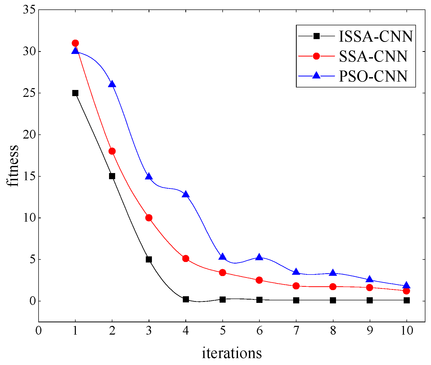It can provide effective representation of images, sequences, and so on [20]. The strength of CNNs lies in their efficient processing of complex data and feature learning capabilities. The proper hyperparameters, such as learning rate and filter size, are crucial to the model performance in CNNs. The sparrow search algorithm (SSA) was proposed in 2020 as a novel swarm intelligence optimization algorithm [21]. It primarily achieves position optimization by emulating the foraging and anti-predatory behaviors of sparrows, aiming to locate the local optimum of a given problem [22]. This study introduces an improved sparrow search algorithm (ISSA) for CNN parameter optimization. ISSA can dynamically adjust these parameters to enhance model generalization and robustness. The proposed approach will be applied to transformer fault diagnosis, showcasing the potential of CNNs optimized with ISSA.

The DGA method primarily utilizes the characteristic gas content for transformer fault diagnosis [23]. However, the composition of dissolved gases in oil is highly complex and uncertain. Therefore, assessing the uncertainty solely based on the decomposed gas content is challenging. This study introduces information entropy [24] as a feature indicator for transformer fault diagnosis. Information entropy, a concept from information theory, measures system uncertainty and information quantity. In transformer diagnosis, information entropy can be employed by analyzing the concentration distribution of dissolved gases, assessing system states. Higher entropy values indicate greater system complexity and uncertainty, potentially indicating underlying faults. 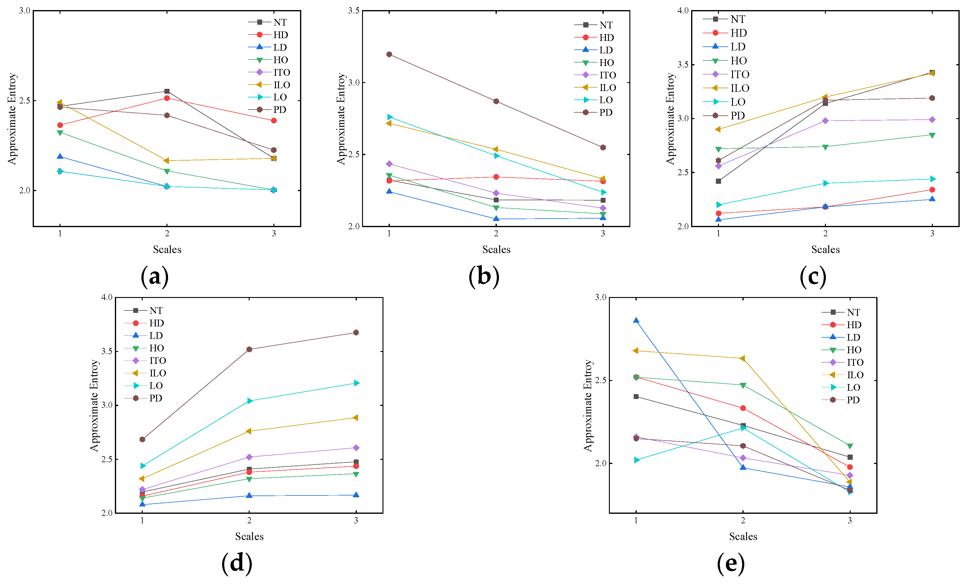Information entropy analysis enhances the understanding of system health, supporting early fault detection and prediction [25]. Approximate entropy, a calculation method for information entropy, is commonly used for time-series data analysis [26]. It assesses system complexity and regularity, revealing patterns or trends in data. Multi-scale approximate entropy considers signal characteristics at different scales, observing how complexity evolves with scale changes [27]. This method contributes to a comprehensive understanding of dynamic signal characteristics. It provides in-depth insights into system behavior across different time scales. Currently, approximate entropy has demonstrated effective applications in various fields, including biosignal analysis [28], short-circuiting arc welding analysis [29], mechanical vibration measurements [30], and environmental monitoring [31]. In transformer diagnosis, this paper attempts to enhance early fault prediction by calculating the multi-scale approximate entropy of dissolved gases in oil, offering a more comprehensive insight into system state changes.

This study initially collects the characteristic gas content of oil-immersed transformers under various fault types, including H₂, CH₄, C₂H₆, C₂H₄, and C₂H₂. Subsequently, the content ratios of different gas types are obtained. The multi-scale approximate entropy values are then calculated through content ratios to assess the gas complexity. Finally, the multi-scale approximate entropy values serve as feature inputs for an optimized CNN-based classifier, deriving diagnostic results. Field data demonstrate the proposed method’s effectiveness and superiority in transformer fault diagnosis.

The structure of this paper is as follows. The principles of the relevant algorithms are detailed in Section 2. Section 3 presents an oil-immersed transformer fault diagnosis model based on multi-scale approximate entropy and optimized CNNs. Section 4 shows the performance of the proposed diagnostic model. Section 5 concludes the paper.

2. Algorithm and Principles

2.1. Multi-Scale Approximate Entropy

2.1.1. Approximate Entropy

Approximate entropy is a non-linear dynamical parameter used to quantify the regularity and unpredictability of fluctuations in a time series. It is represented by a non-negative number that reflects the complexity of a time series, indicating the likelihood of new information occurring in the time series. The more complex the time series, the higher the corresponding approximate entropy.

2.1.2. Algorithm Steps

Let the original signal be a time series containing N data points u(1), u(2), u(3),…, u(N);

Generate a set of vectors with a dimension of m: x(1), x(2), x(3),…, x(N − m + 1), where m represents the length of the window.

$$x(i)=\{u(i),u(i+1),\cdots ,u(i+m-1)\},i\in [1,N-m+1]$$

(1)

Define the distance between x(i) and x(j) as d[x(i), x(j)] to be the maximum of the absolute differences between their corresponding elements.

$$d[x(i),x(j)]=\max [\left|x(i+k)-x(j+k)\right|]$$

(2)

Given a threshold r, for each value of i, count the number of distances d that are less than r, and calculate the ratio of this count to the total number of distances N − m.

$$C_i^m(r)=\frac{1}{N-m}\{d[x(i),x(j)]<r\}$$

(3)

Take the logarithm of $C_i^m(r)$, and then calculate the average across all i in Equation (4).

$${\varphi }^m(r)=\frac{1}{N-m+1}{\displaystyle \sum _{i=1}^{N-m+1}\ln C_i^m(r)}$$

(4)

Increase the dimension by 1 to m + 1, then repeat steps (2) to (5), resulting in $C_i^{m+1}(r)$ and ${\varphi }^{m+1}(r)$.

In theory, the approximate entropy of this sequence is defined as:

$$ApEn(m,r)=\underset{N\to \infty }{\lim }[{\varphi }^m(r)-{\varphi }^{m+1}(r)]$$

(5)

When N is a finite value, the ApEn estimate obtained by following the above steps for a sequence of length N is denoted as:

$$ApEn(m,r,N)={\varphi }^m(r)-{\varphi }^{m+1}(r)$$

(6)

2.1.3. Multi-Scale Approximate Entropy

Multi-scale approximate entropy (MApEn) extends the concept of approximate entropy to multiple time scales. It provides additional perspectives when dealing with data of uncertain time scales. The approximate entropy does not adequately account for different time scales that may exist within a time series. The objective of multi-scale entropy is to assess the complexity of time series.

The fundamental principle of multi-scale entropy involves coarsening or downsampling, primarily analyzing the time series at progressively coarser time resolutions. Coarse-grained data take the average of different numbers of consecutive data points to create signals at different scales. The specific steps are as follows.

When Scale = 1, the coarse-grained data are the original time series.

When Scale = 2, the coarse-grained time series is formed by calculating the average of two consecutive time points, as defined in Equations (7) and (8).

$$y_{1,j}^{(2)}=\frac{x_i+x_{i+1}}{2}$$

(7)

$$y_{2,j}^{(2)}=\frac{x_{i+1}+x_{i+2}}{2}$$

(8)

Similarly, when Scale = n, the coarse-grained time series is formed by taking the average of n consecutive time points, as shown in Figure 1.

The mathematical definition of the above coarse-grained process is as follows.

$$y_j^{(\tau )}=\frac{1}{\tau }{\displaystyle \sum _{i=(j-1)\tau +1}^{j\tau }{X}_i, 1\le j\le \frac{N}{\tau }}$$

(9)

where τ represents the time scale.

2.2. Improved Sparrow Search Algorithm

SSA is a heuristic optimization method inspired by the collective behaviors of sparrow bird populations. It utilizes a combination of individual exploration and information-sharing strategies to address optimization challenges. This algorithm is conceived as an optimization approach that draws inspiration from the foraging and migration patterns of sparrows. However, the SSA algorithm is susceptible to the influence of problem complexity and parameter settings, resulting in slow convergence and low accuracy. In this article, the following improvement strategies are proposed.

(1) This article employs chaotic mapping for the initialization of the SSA population to achieve stable population quality. The generated chaotic sequences are as described in Equation (10).

$$Z_{I+1}^K=\left\{\begin{array}{l}\frac{Z_I^K}{u}, 0\le Z_I^K\le u\\ \frac{1-Z_I^K}{1-u}, u\le Z_I^K\le 1\end{array}\right.$$

(10)

In this context, where K represents the population size and I is the current iteration count, u takes on random values between 0 and 1. The process for initial position generation of sparrow individuals using the chaotic sequence is as follows.

$$X_I^K=(\min )X_I^K+Z_I^K\ast ((\max )X_I^K-(\min )X_I^K)$$

(11)

where $(\min )X_I^K$ and $(\max )X_I^K$ represent the minimum and maximum values of $X_I^K$, respectively.

(2) To prevent being stuck in local optima, this article introduces a non-linearly decreasing weight ${\omega }_{\mathrm{m}}$ in the update of SSA discoverer positions. The calculation formula is as follows.

$${\omega }_m={\omega }_1({\omega }_1-{\omega }_2)(1-\tan \frac{\pi t}{4t_{\max }}\frac{t^2}{t_{\max }^2})$$

(12)

where ω₁ and ω₂ are inertia adjustment parameters with values of ω₁ = 0.9 and ω₂ = 0.4, and t_max represents the maximum number of iterations. The weight has a slower decay at the beginning of iterations, favoring global search for the optimal solution’s position.

(3) This article introduces a mutation strategy to update the contributors. A Gaussian mutation operator is introduced to perturb the global best solution. This can prevent being trapped in local optima. Gaussian mutation operator is defined in Equation (13).

$$X_{gauss}^{t+1}=X_{gauss}^t(1+Gaussian(\alpha ))$$

(13)

where $X_{gauss}^{t+1}$ represents the Gaussian best solution, and $Gaussian(\alpha )$ denotes a random vector following a Gaussian distribution, with a mean of 0 and a variance of 1.

A flowchart of the ISSA is shown in Figure 2.

To validate the performance of ISSA, this study conducted numerical simulation experiments on six selected functions from the Congress on Evolutionary Computation test suite [32]. A comparative analysis was carried out with Particle Swarm Optimization (PSO) [33], Grey Wolf Optimizer (GWO) [34], Gravitational Search Algorithm (GSA) [35], and African Vultures Optimization Algorithm (AVOA) [36]. The six functions and their parameters are listed in

Table 2. Test function parameters.

Test Functions	Search Range	Optimal Value	Dimension
$F_1(x)={\displaystyle \sum _{i=1}^{n-1}\left[100(x_{i+1}-x_i^2)+{(x_i-1)}^2\right]}$	[−30, 30]	0	30
$F_2(x)={\displaystyle \sum _{i=1}^n{\left(\left[x_i+0.5\right]\right)}^2}$	[−100, 100]	0	30
$F_3(x)={\displaystyle \sum _{i=1}^{n}i{x}_i^4}+random[0,1)$	[−1.28, 1.28]	0	30
$F_4(x)=-20\exp \left(-0.2\sqrt{\frac{1}{n}{\displaystyle \sum _{i=1}^n{x}_i^2}}\right)-\exp \left(\frac{1}{n}{\displaystyle \sum _{i=1}^n\cos \left(2\pi x_i\right)}\right)+20+e$	[−32, 32]	0	30
$F_5(x)={\left(\frac{1}{500}+{\displaystyle \sum _{j=1}^{25}\frac{1}{j+{\displaystyle \sum _{i=1}^2{\left(x_i-a_{ij}\right)}^6}}}\right)}^{-1}$	[−65, 65]	1	2
$F_6(x)={{\displaystyle \sum _{i=1}^{11}\left[a_i-\frac{x_1(b_i^2+b_1{x}_2)}{b_i^2+b_1{x}_3+x_4}\right]}}^2$	[−5, 5]	0.000387	4

. The convergence curves of different algorithms are illustrated in Figure 3.

From Figure 3, it can be observed that ISSA exhibits the fastest convergence speed on various test functions, demonstrating significantly better performance compared to PSO, GSA, GWO, and AVOA.

2.3. CNNs

CNNs are a type of deep feedforward neural network with a hierarchical structure. The architecture primarily includes convolutional layers, pooling layers, activation layers, and fully connected layers.

2.3.1. Convolutional Layer

The main role of the convolutional layer in CNNs is to perform feature extraction on the input. The convolutional kernels in different layers have varying sizes, allowing the network to capture features of different scales. As a result, CNNs can extract multi-scale feature information. The calculation formula for the output value $a_j^l$ of the jth unit in convolutional layer l is as follows.

$$a_j^l=f(b_j^l+{\displaystyle \sum _{i\in M_j^l}{a}_j^{l-1}\ast k_{ij}^l})$$

(14)

where $M_j^l$ represents the selected set of input feature maps, and k represents the learnable convolutional kernel.

2.3.2. Pooling Layer

Pooling operations are performed independently on each subset of data.. The purpose of pooling is to gradually reduce the spatial dimensions of the data volume. This helps reduce the number of parameters in the network, saving computational resources effectively. Pooling is commonly used during upsampling and downsampling processes. It has no learnable parameters. The calculation of activation value in pooling layer l is based on Equation (15).

$$a_j^l=f(b_j^l+{\beta }_j^{l-1}down(a_j^{l-1},M^l))$$

(15)

where down(.) represents pooling function, $b_j^l$ is the bias, ${\beta }_j^l$ means the multiplicative residual, and M^l represents the size of the pooling window.

2.3.3. Activation Layer

CNNs are composed of multiple layers of composite functions. Rectified Linear Unit (ReLU) is a widely used activation function in CNNs. Its sparse representation can accelerate learning and simplify models. The mathematical expression of the ReLU function is as follows.

$$f(p)=\max (0,p)$$

(16)

For an input p, the ReLU function returns an output equal to the maximum value between p and 0. If p is greater than or equal to 0, the output is p itself; otherwise, the output is 0.

2.3.4. Fully Connected Layer

The parameters in the fully connected layer include the total number of fully connected layers and the number of neurons in each individual layer. Increasing the width of the fully connected layer and the number of layers can enhance the model’s non-linear expressive power.

2.4. Optimized CNNs with ISSA

The basic process of CNNs based on ISSA is illustrated in Figure 4.

3. Power Transformer Fault Diagnosis Based on Multi-Scale Approximate Entropy and Optimized Deep Convolutional Networks

This study utilizes the optimized convolutional neural network for the analysis of dissolved gases in transformer oil. Initially, eight types of dissolved gases in transformer oil are collected. Subsequently, the gas contents are numerically labeled and normalized. The multi-scale approximate entropy is employed for feature extraction on the pre-processed data. Finally, the extracted features are fed into the optimized convolutional neural network for fault diagnosis. The diagnostic process is illustrated in Figure 5.

4. Case Study Analysis

4.1. Data Preprocessing

The raw data used in this study consist of actual measurements of dissolved gases in transformer oil from a certain substation, totaling 555 sets. Some of the transformer parameters are present in

Table 3. Transformer parameters.

Type	Parameters
Substation Voltage Level	750 kV
Transformer Model	ODFPS-500000/750
Production Time	June 2018
Commissioning Date	14 May 2019
Main Transformer Cooler Model	YF-400

.

Each set of data includes five features along with the corresponding eight data types, including normal type (NT), high-energy discharge (HD), low-energy discharge (LD), high-temperature overheating (HO), intermediate-temperature overheating (ITO), intermediate- to low-temperature overheating (ILO), low-temperature overheating (LO), and partial discharge (PD). Some of the gas chromatography data are presented in

Table 4. Transformer oil chromatography data.

Sequence	H2	CH4	C2H6	C2H4	C2H2	Data Type
1	0.00	1.78	1.02	2.16	0.42	NT
2	130.00	98.00	7.00	56.00	65.00	HD
3	428.00	1660.00	533.00	4094.00	11.40	HO
4	97.81	15.87	2.71	8.10	24.36	LD
…	…	…	…	…	…	…
555	17.30	3.20	6.50	4.50	0.40	PD

.

Due to significant differences in gas content values corresponding to different fault types, this study performs standardization on the gas contents using Equation (17). The processed data are presented in

Table 5. Normalized results.

Sequence	H2	CH4	C2H6	C2H4	C2H2	Data Type
1	0.000	0.824	0.472	1.000	0.194	NT
2	1.000	0.750	0.039	0.422	0.492	HD
3	0.104	0.405	0.129	1.000	0.002	HO
4	1.000	0.138	0.000	0.057	0.228	LD
…	…	…	…	…	…	…
555	1.000	0.166	0.361	0.243	0.000	PD

.

$$x^{\prime }=\frac{x-\min (x)}{\max (x)-\min (x)}$$

(17)

Due to the correlation between transformer fault types and the corresponding gas content ratios, gas ratios are commonly used as input data in transformer fault diagnosis. In this work, 21 gas ratios were obtained, as shown in

Table 6. 21 Gas ratios.

Index	Gas Ratios	Index	Gas Ratios	Index	Gas Ratios
1	CH4/H2	8	C2H2/C2H4	15	C2H6/C2H4
2	C2H4/H2	9	H2/TH	16	CH4/TD
3	C2H6/ALL	10	C2H6/H2	17	C2H2/TD
4	C2H6/CH4	11	C2H6/TH	18	C2H2/CH4
5	H2/ALL	12	C2H4/ALL	19	C2H2/H2
6	C2H2/C2H6	13	CH4/TH	20	C2H2/TH
7	C2H4/TD	14	CH4/ALL	21	C2H2/ALL

.

In Table 6, ALL = CH₄ + C₂H₆ + C₂H₄ + C₂H₂ + H₂, TD = CH₄ + C₂H₄ + C₂H₂, TH = CH₄ + C₂H₆ + C₂H₄ + C₂H₂. Partial gas ratio data obtained after calculation are shown in

Table 7. Partial gas ratio.

1	2	3	4	5	6	7	8	9	10	11	12	13	14	15	16	17	18	19	20	21	Data Type
178	102	42	0.2	0.2	0.4	0.5	0.6	0.3	0.4	0.2	0.1	0.0	0.1	0.5	0.4	0.0	0.3	0.2	178	102	NT
0.8	0.1	0.5	1.2	0.7	9.3	0.1	0.1	0.4	0.2	0.0	0.3	0.6	0.3	0.3	0.4	0.4	0.3	0.0	0.8	0.1	HD
3.9	1.2	0.0	0.0	0.0	0.0	0.1	0.3	0.3	0.7	0.1	0.0	0.1	0.0	0.7	0.3	0.1	0.2	0.1	3.9	1.2	HO
0.2	0.0	0.2	3.0	1.5	9.0	0.3	0.2	0.3	0.2	0.1	0.5	1.9	0.5	0.2	0.3	0.7	0.1	0.0	0.2	0.0	LD
1.3	0.2	0.0	0.0	0.0	0.0	0.2	0.1	0.6	0.4	0.1	0.0	0.4	0.0	0.4	0.6	0.3	0.4	0.0	1.3	0.2	LO
1.7	0.4	0.0	0.0	0.0	0.0	0.2	0.2	0.4	0.5	0.1	0.0	0.2	0.0	0.6	0.4	0.2	0.3	0.1	1.7	0.4	ITO
1.2	1.0	0.0	0.0	0.0	0.0	0.8	0.9	0.3	0.4	0.3	0.0	0.3	0.0	0.5	0.5	0.2	0.3	0.2	1.2	1.0	ILO
…	…	…	…	…	…	…	…	…	…	…	…	…	…	…	…	…	…	…	…	…	…
0.2	0.4	0.0	0.1	0.1	0.1	1.4	2.0	0.2	0.3	0.4	0.0	1.2	0.0	0.6	0.4	0.5	0.1	0.2	0.1	0.0	PD

.

4.2. Feature Extraction

To extract valuable feature information from the aforementioned gas ratios, multi-scale approximate entropy is introduced to extract characteristic parameters from the gas ratio data. With an approximate entropy scale set to 10, the obtained approximate entropy values for different types of gas contents are illustrated in Figure 6.

Figure 6 shows that when the scale is greater than 6, the approximate entropy values for different transformer faults are relatively similar, exhibiting the same changing trend. At scale values of 4, 5, and 6, there still exist some fault types with similar approximate entropy values. However, at a scale value of 3, the differences in approximate entropy values among different faults become more distinct. Considering that a low scale may lead to the loss of sample information, the scale is set to 3 in this study.

Taking into account the impact of different embedding dimensions on entropy values, the embedding dimensions range from 2 to 6. Figure 7 presents the comparative results for different fault types under different embedding dimensions.

The impact of the embedding dimension for different fault types is evident from Figure 7. When m takes values of 2, 3, 4, and 6, there is a drastic fluctuation in approximate entropy values, leading to potential confusion between different fault types. However, when m is set to 5, the approximate entropy values for different fault types exhibit a more gradual change with increasing scales. Therefore, m is set to 5. Partial results are presented in

Table 8. Partial multi-scale entropy value results.

Scale 1	Scale 2	Scale 3	Data Type
3.41	2.85	2.67	HO
3.36	2.8	2.35	LD
2.71	2.86	2.96	HO
3.40	2.89	2.59	ILO
3.40	2.98	2.69	PD
3.34	3.07	2.96	PD
…	…	…	…
3.44	3.11	3.04	HD

.

4.3. Optimized CNNs with ISSA

This section utilizes the extracted data to train a CNN model. Initially, the ISSA optimization method is employed to fine-tune the CNN hyperparameters, with a maximum training iteration set to 10. The discoverer’s proportion in the population is determined to be 20%. The parameters are presented in

Table 9. CNN hyperparameters.

Hyperparameters	Range	Initial Parameters	Optimized Parameters
learning rate	0.001~0.01	0.01	0.0042
number of iterations	10~50	25	35
batch size	16~256	64	34
kernel size of convolutional layer 1	1~16	5	10
kernel number of convolutional layer 1	1~20	20	20
kernel size of convolutional layer 2	1~16	10	6
kernel number of convolutional layer2	1~20	20	20
neuron in fully connected layer 1	1~50	30	25
neuron in fully connected layer 2	1~50	10	39

.

Figure 8 depicts the fitness curves obtained through testing with PSO-CNN, SSA-CNN, and ISSA-CNN, respectively.

From Figure 8, it is evident that, compared to PSO-CNN and SSA-CNN, ISSA-CNN converges more rapidly to a stable fitness value, indicating its superior optimization effectiveness.

4.4. Results Analysis

This study analyzes 555 sets of transformer data, comparing the situations before and after feature extraction. Five-fold cross-validation is employed in this study, where the sample data are randomly divided into five equal parts, namely D1, D2, D3, D4, and D5. Each part is used as a test set in turn, while the remaining four parts serve as training sets. The testing results are illustrated in Figure 9. Raw data represent the original data of 21 gas ratios, while MApEn denotes the multi-scale approximate entropy values. The memory consumption before and after feature extraction is presented in Figure 10. The memory consumption of the model before and after optimization with ISSA is presented in Figure 11.

Figure 9 indicates that after utilizing multi-scale approximate entropy for feature extraction in transformer data, the diagnostic results for different partitions show better performance compared to the diagnostic performance before feature extraction. It indicates that the feature extraction method in this study can collect valuable transformer data information and eliminate easily confused redundant information.

Figure 10 shows that the memory consumption of the model in processing data is much lower after feature extraction compared to that before feature extraction. This indicates that the feature extraction method in this study significantly improves the efficiency of diagnostic operations.

Figure 11 indicates that the memory consumption of the model during fault diagnosis is much lower after ISSA optimization. This means that the ISSA method significantly improves the efficiency of diagnostic operations.

In order to thoroughly validate the superiority of the proposed transformer fault diagnostic model, three algorithms, including BPNN, ELM, and CNN, are introduced in this study for comparative analysis. The confusion matrix obtained through a five-fold cross-validation method is presented in Figure 12.

In Figure 12, it is evident that different diagnostic methods yield significantly different diagnostic results. As seen in Figure 12a, the diagnostic performance of the BPNN method is relatively poor. Although it accurately identifies data with ITO, it struggles to recognize other types of transformer faults. In Figure 12b, the ELM method improves the diagnostic accuracy but still exhibits noticeable misjudgments, making it difficult to differentiate between ITO and ILO. The results in Figure 12c indicate that the CNN, compared to the first two algorithms, achieves an overall improvement in recognition accuracy. However, there are still clear misjudgments in identifying fault labels. In Figure 12d, it can be observed that the CNN classification model optimized through ISSA demonstrates excellent recognition performance, meeting the engineering requirements.

To provide a comprehensive assessment of the proposed model’s performance, this paper employs accuracy, precision, recall, F1-score, and Kappa coefficient for analysis. Accuracy is a fundamental metric for evaluating the performance of a classification model, measuring the ratio of correctly classified samples to the total number of samples. Precision represents the proportion of true-positive samples among those predicted as positive. Recall indicates the ratio of samples predicted as positive to all actual positive samples. F1-score is a metric that combines precision and recall, representing their harmonic mean. The Kappa coefficient is a statistical measure of classification model performance, considering the difference between the model’s performance and random classification. The Kappa coefficient value ranges from −1 to 1, where 1 signifies perfect agreement, 0 indicates no difference from random classification, and −1 denotes complete disagreement. The calculation method is as shown in Equations (18)–(23).

$$Accuracy=\frac{TP+TN}{TP+TN+FP+FN}$$

(18)

$$Precision=\frac{TP}{TP+FP}$$

(19)

$$Recall=\frac{TP}{TP+FN}$$

(20)

$$F1-score=\frac{2*Precision*Recall}{Precision+Recall}$$

(21)

$$Kappa=\frac{Accuracy-P(E)}{1-P(E)}$$

(22)

where TP represents true positive, TN represents true negative, FP represents false positive, and FN represents false negative. P(E) is the expected accuracy, calculated in Equation (23), representing the performance under random conditions.

$$P(E)=\frac{(TP+FP)*(TP+FN)+(TN+FN)*(TN+FP)}{{(TP+TN+FP+FN)}^2}$$

(23)

The diagnostic results for different methods are illustrated in Figure 13. The box in the figure represents the interquartile range from the upper quartile to the lower quartile. The upper and lower whiskers, respectively, depict the maximum and minimum values. The median point represents the middle value, indicating the average level of the metrics calculated by this method.

Figure 13a reveals significant differences in fault accuracy among the four diagnostic methods, and the ISSA-CNN method exhibits a distinct advantage compared to the other three methods. The diagnostic results in Figure 13b indicate that ISSA-CNN achieves higher precision in terms of maximum, minimum, and average values, demonstrating superior recognition performance within the limited transformer data range. The results in Figure 13c suggest that the recall rate of the proposed method is higher, indicating a greater number of correctly predicted samples and a clear advantage in diagnostic effectiveness. As shown in Figure 13d, the F1-scores obtained by ISSA-CNN are distributed above 85%, indicating excellent generalization performance. Figure 13e demonstrates that the Kappa coefficient of ISSA-CNN has a minimum value and overlapping boxes, indicating a stable distribution range and high classification accuracy.

5. Conclusions

Building upon the analysis of dissolved gases in transformer oil, this study proposes the ISSA-CNN model for transformer fault diagnosis. The conclusions are as follows.

• This study introduces an improved sparrow search algorithm that incorporates enhancement strategies in population initialization and position updating. The effectiveness of the enhanced algorithm is validated through optimizing test functions. The algorithm is then applied to optimize the hyperparameters of CNNs. Comparative analysis with different optimization algorithms and validation on the DGA dataset demonstrates its superiority.
• This study analyzes eight different types of transformer oil and gas data, deriving 21 gas ratios. Subsequently, multi-scale approximate entropy is calculated for these gas ratio contents. The uncertainty of dissolved gases in transformer oil is represented by entropy values, and the multi-scale approximate entropy values are used as feature vectors input into the optimized CNN diagnostic model. The results indicate that the extracted multi-scale approximate entropy can effectively characterize dissolved gas contents and improve the diagnostic effectiveness.
• To verify the effectiveness and superiority of the proposed method, this study compares it with BPNN, ELM, and CNNs. The results show that the ISSA-CNN transformer fault diagnosis model outperforms the other three methods in terms of accuracy, recall rate, precision, F1-score, and Kappa coefficient. This indicates that the proposed method has good generalization performance and demonstrates favorable application effects in transformer fault diagnosis.

In the future: the authors will attempt to collect more on-site transformer fault data to validate the effectiveness and practicality of the proposed model. Additionally, further improvements can be made to better optimize the parameters of the convolutional neural network and enhance the robustness and stability of the model.

References

1. Deng, Y.; Ruan, J.; Dong, X.; Huang, D.; Zhang, C. Inversion detection method of oil-immersed transformer abnormal heating state. IET Electr. Power Appl. 2022, 17, 134–148. [Google Scholar] [CrossRef]
2. Wang, K.; Fu, Y.; Kong, D.; Wang, S.; Li, L. First-principles insight into adsorption behavior of a Pd-doped PtTe2 monolayer for CO and C2H2 and the effect of an applied electric field. J. Phys. Chem. Solids 2023, 177, 111289. [Google Scholar] [CrossRef]
3. Zeng, W.; Cao, Y.; Feng, L.; Fan, J.; Zhong, M.; Mo, W.; Tan, Z. Hybrid CEEMDAN-DBN-ELM for online DGA serials and transformer status forecasting. Electr. Power Syst. Res. 2023, 217, 109176. [Google Scholar] [CrossRef]
4. Wakimoto, K.; Shigemori, K. Interpretation of Dissolved Gas Analysis (DGA) for Palm Fatty Acid Ester (PFAE)-Immersed Transformers. Meiden Rev. Int. Ed. 2022, 186, 14–17. [Google Scholar]
5. Afrida, Y.; Fitriono. Analisa Kondisi Minyak Trafo Berdasarkan Hasil Uji Dissolved Gas Analisys Pada Trafo Daya #1 Di PT.PLN (PERSERO) GARDU INDUK KOTABUMI. Electrician 2022, 2, 119–126. [Google Scholar]
6. Guo, C.; Zhang, Q.; Zhang, R.; He, X.; Wu, Z.; Wen, T. Investigation on gas generation characteristics in transformer oil under vibration. IET Gener. Transm. Distrib. 2022, 16, 5026–5040. [Google Scholar] [CrossRef]
7. Zhou, Y.; Yang, X.; Tao, L.; Yang, L. Transformer Fault Diagnosis Model Based on Improved Gray Wolf Optimizer and Probabilistic Neural Network. Energies 2021, 14, 3029. [Google Scholar] [CrossRef]
8. Sarma, G. Multilevel SVM and AI based Transformer Fault Diagnosis using the DGA Data. J. Inform. Electr. Electron. Eng. 2021, 2, 1–16. [Google Scholar] [CrossRef]
9. Mani, G.; Jerome, J. Intuitionistic Fuzzy Expert System based Fault Diagnosis using Dissolved Gas Analysis for Power Transformer. J. Electr. Eng. Technol. 2014, 9, 2058–2064. [Google Scholar] [CrossRef]
10. Han, X.; Ma, S.; Shi, Z.; An, G.; Du, Z.; Zhao, C. Transformer Fault Diagnosis Technology Based on Maximally Collapsing Metric Learning and Parameter Optimization Kernel Extreme Learning Machine. IEEJ Trans. Electr. Electron. Eng. 2022, 17, 665–673. [Google Scholar] [CrossRef]
11. Beghi, A.; Brignoli, R.; Cecchinato, L.; Menegazzo, G.; Rampazzo, M.; Simmini, F. Data-driven fault detection and diagnosis for hvac water chillers. Control Eng. Pract. 2016, 53, 79–91. [Google Scholar] [CrossRef]
12. Qin, S.J. Data-driven fault detection and diagnosis for complex industrial processes. IFAC Proc. Vol. 2009, 42, 1115–1125. [Google Scholar] [CrossRef]
13. Sulaiman, N.A.; Chuink, K.W.; Zainudin, M.N.; Yusop, A.M.; Sulaiman, S.F.; Abdullah, P. Data-driven fault detection and diagnosis for centralised chilled water air conditioning system. Prz. Elektrotech. 2022, 98, 135378. [Google Scholar] [CrossRef]
14. Yin, S.; Wang, G.; Karimi, H.R. Data-driven design of robust fault detection system for wind turbines. Mechatronics 2014, 24, 298–306. [Google Scholar] [CrossRef]
15. Hossein, D. A machine-learning architecture for sensor fault detection, isolation, and accommodation in digital twins. IEEE Sens. J. 2023, 23, 2522–2538. [Google Scholar]
16. Papa, U.; Fravolini, M.L.; Core, G.D.; Papa, U.; Valigi, P.; Napolitano, M.R. Data-driven schemes for robust fault detection of air data system sensors. IEEE Trans. Control Syst. Technol. 2017, 99, 234–248. [Google Scholar]
17. Darvishi, H.; Ciuonzo, D.; Eide, E.R.; Rossi, P.S. Sensor-fault detection, isolation and accommodation for digital twins via modular data-driven architecture. IEEE Sens. J. 2023, 23, 29877–29891. [Google Scholar] [CrossRef]
18. Tang, M.; Zhang, J.; Liu, Y.; Zhao, Y.; Li, Y. The optimal control of floor radiant heating system based on deep reinforcement learning. J. Northeast. Electr. Power Univ. 2022, 42, 14–25. [Google Scholar]
19. Choudhary, A.; Mishra, R.K.; Fatima, S.; Panigrahi, B. Multi-input CNN based vibro-acoustic fusion for accurate fault diagnosis of induction motor. Eng. Appl. Artif. Intell. 2023, 120, 105872. [Google Scholar] [CrossRef]
20. Asif, S.; Kartheeban, K. CNN-RNN Algorithm-based Traffic Congestion Prediction System using Tri-Stage Attention. Int. J. Sens. Wirel. Commun. Control 2023, 13, 89–98. [Google Scholar] [CrossRef]
21. Xue, J.k. Research and Application of a Novel Swarm Intelligence Optimization Technique: Sparrow Search Algorithm. Donghua Univ. 2020, 8, 22–34. [Google Scholar]
22. Ou, Y.; Yu, L.; Yan, A. An Improved Sparrow Search Algorithm for Location Optimization of Logistics Distribution Centers. J. Circuits Syst. Comput. 2023, 32, 2350150. [Google Scholar] [CrossRef]
23. Article, I. Dissolved gas analysis: Early fault indication and trend analysis. Transform. Mag. 2023, 10, 89–95. [Google Scholar]
24. Núñez, J.A.; Cincotta, P.M.; Wachlin, F.C. Information entropy. Celest. Mech. Dyn. Astron. 1996, 64, 43–53. [Google Scholar] [CrossRef]
25. Han, J.J.; Yoon, H.Y.; Pradhan, O.J.; Wu, T.; Wen, J.; O’neill, Z.; Candan, K.S. A cosine-based correlation information entropy approach for building automatic fault detection baseline construction. Sci. Technol. Built Environ. 2022, 28, 1138–1149. [Google Scholar]
26. Pincus, S. Approximate entropy (ApEn) as a complexity measure. Chaos 1995, 5, 110–117. [Google Scholar] [CrossRef]
27. Singh, V.; Gupta, A.; Sohal, J.S.; Singh, A. Multi-Scale Fractal Dimension to Quantify Heart Rate Variability and Systolic Blood Pressure Variability: A Postural Stress Analysis. Fluct. Noise Lett. 2019, 18, 1950019. [Google Scholar] [CrossRef]
28. Parthasarathy, S.; Maresova, P.; Rajagopal, K.; Namazi, H. Analysis of the Changes in the Brain Activity Between Rest and Multitasking Workload by Complexity-Based Analysis of Eeg Signals. Fractals 2023, 31, 2350136. [Google Scholar] [CrossRef]
29. Cao, B.; Lü, X.Q.; Zeng, M.; Wang, Z.M.; Huang, S.S. Approximate entropy analysis of current in short-circuiting arc welding. Acta Phys. Sin. 2006, 55, 1696–1705. [Google Scholar] [CrossRef]
30. An, X.; Li, C.; Zhang, F. Application of adaptive local iterative filtering and approximate entropy to vibration signal denoising of hydropower unit. J. Vibroeng. 2016, 18, 4299–4311. [Google Scholar] [CrossRef]
31. Ahmad, S.; Agrawal, S.; Joshi, S.; Taran, S.; Bajaj, V.; Demir, F.; Sengur, A. Environmental sound classification using optimum allocation sampling based empirical mode decomposition. Phys. A Stat. Mech. Its Appl. 2020, 537, 122613. [Google Scholar] [CrossRef]
32. Mandziuk, J.; Abbass, H. Conference Report on 2021 IEEE Congress on Evolutionary Computation. IEEE Comput. Intell. Mag. 2021, 16, 5–8. [Google Scholar] [CrossRef]
33. Gargiulo, L.; Ibba, L.; Malagoli, P.; Amoruso, F.; Argenziano, G.; Balato, A.; Bardazzi, F.; Burlando, M.; Carrera, C.G.; Damiani, G.; et al. A Risankizumab Super Responder Profile Identified by Long-term Real-Life Observation- IL PSO (ITALIAN LANDSCAPE PSORIASIS). J. Eur. Acad. Dermatol. Venereol. JEADV 2023, 38, e113–e116. [Google Scholar] [CrossRef]
34. Ma, S.; Fang, Y.; Zhao, X.; Liu, Z. Multi-swarm improved Grey Wolf Optimizer with double adaptive weights and dimension learning for global optimization problems. Math. Comput. Simul. 2023, 205, 619–641. [Google Scholar] [CrossRef]
35. Salajegheh, F.; Salajegheh, E.; Shojaee, S. An enhanced approach for optimizing mathematical and structural problems by combining PSO, GSA and gradient directions. Soft Comput. 2022, 26, 11891–11913. [Google Scholar] [CrossRef]
36. Gürses, D.; Mehta, P.; Sait, S.M.; Yildiz, A.R. African vultures optimization algorithm for optimization of shell and tube heat exchangers. Mater. Test. 2022, 64, 1234–1241. [Google Scholar] [CrossRef]
Figure 1. Schematic of the coarse-grained process.
Entropy 26 00186 g001
Figure 2. The flowchart of ISSA.
Entropy 26 00186 g002
Figure 3. Fitness curves of different algorithms. (a) F1; (b) F2; (c) F3; (d) F4; (e) F5; (f) F6.
Entropy 26 00186 g003aEntropy 26 00186 g003b
Figure 4. The process of CNNs based on ISSA.
Entropy 26 00186 g004
Figure 5. Power transformer fault diagnosis procedure.
Entropy 26 00186 g005
Figure 6. Approximate entropy values varying with different scales.
Entropy 26 00186 g006
Figure 7. Comparison with different embedding dimensions. (a) m = 2; (b) m = 3; (c) m = 4; (d) m = 5; (e) m = 6.
Entropy 26 00186 g007
Figure 8. Fitness curve of different optimization methods.
Entropy 26 00186 g008
Figure 9. Test results.
Entropy 26 00186 g009
Figure 10. The memory consumption before and after feature extraction.
Entropy 26 00186 g010
Figure 11. The memory consumption before and after optimization via ISSA.
Entropy 26 00186 g011
Figure 12. Diagnostic accuracy of different algorithms. (a) BPNN; (b) ELM; (c) CNN; (d) ISSA-CNN.
Entropy 26 00186 g012aEntropy 26 00186 g012b
Figure 13. Different methods of assessing results and analysis. (a) Accuracy; (b) precision rate; (c) recall rate; (d) F1-score; (e) Kappa coefficient.
Entropy 26 00186 g013