Word Length in Political Public Speaking: Distribution and Time Evolution

Abstract

In this paper, word length in the texts of public speeches by USA and UK politicians is analyzed. More than 300 speeches delivered over the past two hundred years were studied. It is found that the lognormal distribution better describes the distribution of word length than do the Weibull and Poisson distributions, for example. It is shown that the length of words does not change significantly over time (the average value either does not change or slightly decreases, and the mode slightly increases). These results are fundamentally different from those obtained previously for sentence lengths and indicate that, in terms of quantitative linguistic analysis, the word length in politicians’ speech has not evolved over the last 200 years and does not obey the principle of least effort proposed by G. Zipf.

1. Introduction

Natural languages have been one of the most important subjects of science for a long time. However, the interest in language research has flared up with renewed vigor in recent times due to the development of computer technology, general digitalization, development of artificial intelligence systems, etc. One of the scientific areas demonstrating a new impetus for development is quantitative linguistics. Here, quantitative statistical methods of analysis are used to study texts and speeches, which helps to gain a deeper understanding of the structure and evolution of language. By transforming linguistic objects of natural language into numbers according to certain rules, quantitative linguistics strives, on the basis of statistical analysis, to formulate general laws according to which language functions. There are a number of achievements along this path, three of which are as follows: Zipf’s law: the frequency of words is inversely proportional to their rank in frequency lists. Brevity law: the more frequently a word is used, the “shorter” that word tends to be. Menzerath–Altmann law: the sizes of the constituents of a construction decrease with the increase in size of the construction under study, and vice versa [1,2].

It is well known [3,4] that homogeneous and representative datasets (collections of texts) should be used to detect linguistic laws, since even the genre of the text [5,6,7], not to mention the time of its writing, can influence the results obtained. An important dataset for study is the texts of politicians’ public speeches. These texts are well documented over an interval of sufficient length and “ought to be fairly consistent in genre and register” [8]. An important feature of political speeches is that for the most part they are carefully prepared for perception and effective impact on the average mass listener living in a certain time epoch. Therefore, despite the specific genre, political speeches are an excellent object for studying the laws and evolution of language.

The study of politicians’ public speeches using the methods of quantitative linguistics has been previously carried out in works [8,9,10,11,12]. In particular, [8] analyzes the inaugural speeches of USA presidents and notes that the average length of sentences has monotonically decreased over 200 years, and in total has decreased by approximately 50%. In [9], this conclusion for the USA was confirmed and also generalized to public speeches by members of UK parliamentary parties in the period from 1900 to 2000. It was found in [9] that the frequency distribution of sentence lengths during public speaking in the USA and the UK is best described not by the lognormal distribution, but by the Weibull distribution. A similar distribution and reduction in the length of sentences over time was associated in [9] with the principle of least effort proposed by G. Zipf [4,13,14]. The formulation of this principle is as follows: “… the person will strive to minimize the probable average rate of his work-expenditure (over time). And in so doing he will be minimizing his effort. … Least effort, therefore, is a variant of least work.”.

Will the length of words, rather than sentences, also obey the principle of least effort for the same public speeches of politicians, i.e., have Weibull distributions and decrease over time?

This is a very interesting and controversial issue. Indeed, according to Zipf’s law and the brevity law, the power function describes the distribution of word lengths [13,14,15] and considering the Weibull distribution is an unnecessary complication. However, a question arises regarding the validity of these laws when considering words of arbitrary length. For example, according to studies [15] conducted for English and Swedish, only words containing more than three letters follow this law and without a lower bound on word length, the distribution of word lengths should be more complex. Both discrete distributions (especially Poisson) [4,5] and continuous distributions (in particular, lognormal and gamma distributions) [13,15,16,17,18] have been previously proposed in the literature as possible options. Regarding the temporal behavior of average word length, research results are very contradictory [5]. Thus, according to the Menzerath–Altmann law, as the length of sentences calculated in words decreases, the length of the words should increase on average. From the studies of politicians’ public speeches [8,9,10], the sentence length, as mentioned above, decreases significantly over time. However, according to [8], the length of the word does not increase, but rather decreases slightly (by about 5% over the last century). Note that for other genres of text, there has been a slight increase in the average word length over several centuries for Arabic [7], as well as for English and Russian throughout the nineteenth and most of the twentieth century [11] (however, according to [11], since the end of the twentieth century, there has been a decrease in the average word length). Other studies of changes in average word length over time can be found in [5,11,19]; their results are extremely contradictory. Thus, as seen here, there is no answer to the question formulated above. The purpose of this paper is to attempt to answer it within quantitative linguistics.

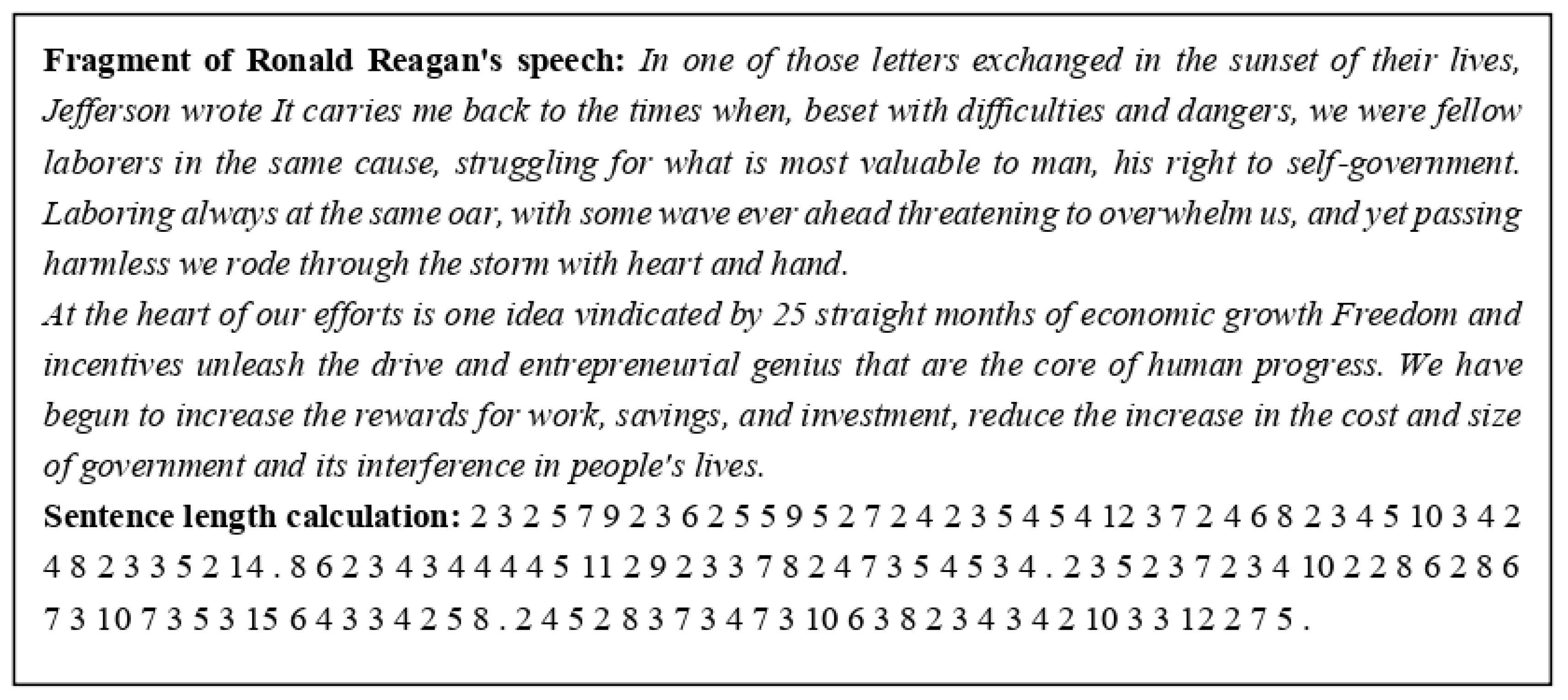
2. Data for Analysis

The choice of public speeches of politicians in the USA and the UK was determined by the availability of speeches in digital archives, as well as by a desire for homogeneity of texts by genre and uniformity in distribution over time.

We analyzed text transcripts of 88 speeches by USA presidents from 1789 to 2021 (including 59 inaugural addresses), available in [20,21]. Six speeches were made in the 18th century, 51 speeches were made in the 19th century, 25 in the 20th century, and 6 in the 21st century. For the 18th and 19th centuries, speeches by USA presidents were both inaugural and other speeches. These speeches were made in 1789, 1793, 1796–1798, 1801, 1803, 1805, 1809, 1812, 1813, 1815, 1817, 1821, 1825, 1827, 1829, 1833, 1837–1839, 1841, 1842, 1845, 1846, 1848–1851, 1853, 1854, 1856, 1857, 1861, 1864, 1865, 1869, 1873, 1875–1877, 1879, 1881, 1885, 1889, 1893, 1895, 1897. For the 20th and 21st centuries, only inaugural addresses were used (except for 1968, where an additional speech by President Johnson was used); as a result, they are uniformly distributed every four years 1901–2021.

For the UK, transcripts of 247 speeches were analyzed for the period from 1808 to 2018. These speeches are available in [22,23]. Initially, only the speeches of UK party leaders were considered, but they only covered the period from 1895 to 2018. To extend the temporal coverage, speeches by queens and kings have been added, as well as some additional speeches by party members in Parliament. As a result, 19 speeches were analyzed for the 19th century (they belonged to 1808, 1814, 1814, 1815, 1817, 1819, 1827, 1830, 1837, 1842, 1853, 1868, 1877, 1893, 1895, 1896, 1897, 1897, 1899), 170 for the 20th century (1900–1913, 1917–1930, 1932–1937, 1941–1943, 1945–1951, 1955–1958, 1960–1999), and 58 speeches (2000–2018) for the 21st century.

The word length was determined by the number of letters from space to space. This approach is not universal, but it is widely used [19,24]. It is known that there is still no universal, generally accepted unit for measuring word length (number of syllables, number of letters, breath groups, etc.). The choice of such a unit is made on the basis of the problem statement [4,19,24]. At the moment, we cannot be completely sure that the method of measuring word length does not affect the results obtained. So, in [25], it is stated that: “There can be no a priori decision as to what a word is, or in what units word length can be measured. Meanwhile, in contemporary theories of science, linguistics is no exception to the rule: there is hardly any science which would not acknowledge, to one degree or another, that it has to define its object, first, and that constructive processes are at work in doing so. What has not yet been studied is whether there are particular dependencies between the results obtained on the basis of different measurement units; it goes without saying that, if they exist, they are highly likely to be language-specific.”.

Word length calculation was performed automatically using the developed and tested computer program (see an example of such calculation in Figure 1).

As can be seen from Figure 1, the software we use counts digits, and this can often be incorrect in terms of the length of the spoken words that these digits represent. We did not change the software algorithm since this is a rather non-trivial computer task. But the most important reason for our inaction in this matter is that the error introduced by these digits into the results obtained in the paper turns out to be negligibly. This is due to the fact that the share of the number of digits in relation to the total number of words in the studied political speeches is very small. In the speech, a fragment of which is presented in Figure 1, this share is 0.003, and the highest share in the studied speeches was about 0.004. The statistical quantities studied below are not sensitive to this influence. This software was previously used to calculate sentence lengths as well [9]. Therefore, the dots in the text are saved after processing, as is demonstrated in the fragment below. These dots have no effect on word length processing.

The average speech length in words was approximately 2800 for the USA and 5100 for the UK. As can be seen from Figure 2, in the vast majority of cases the number of words for each speech is more than 1000. This is a very good sample size for a reliable analysis. The difference in the average number of words for the USA and the UK is due to political tradition and historical reasons. This difference is not the subject of this article and does not affect the results presented below.

In further analysis, word length will be treated as a random variable. This term is used in the sense of mathematical statistics. One may wonder whether such an assumption can be used when the texts of political speeches are usually carefully prepared. The answer is yes, for two reasons. The first reason is that when preparing speeches, one does not consider the length of the words, but primarily their content and meaning. The second reason is that even if writers of political speeches paid special attention to the length of the words used (and, for example, considered the Menzerath–Altmann law or various readability indexes), many other controlled and uncontrolled factors, such as political, cultural, historical, psychological, etc., would have various multidirectional effects on the choice of words and therefore, from the point of view of mathematical statistics, word length would be random.

Statistical analysis was carried out in widespread professional commercial software MATLAB R2020 (The MathWorks). Distribution parameters were calculated using the Levenberg–Marquardt algorithm implemented in MATLAB. The commercial software Statistica 12.0 (TIBCO Software) was used to visualize the results and to validate and verify several calculations. The data (year of the speech and values corresponding to the processed word lengths of speeches) are open access [26].

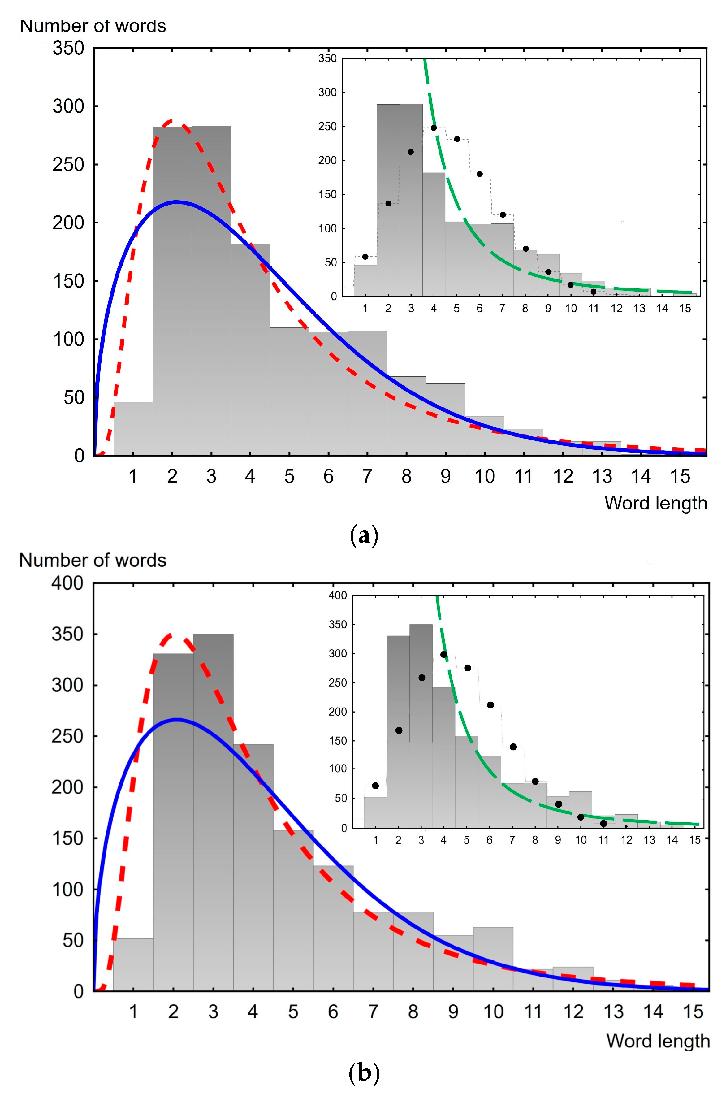
3. Analysis of the Word Length Distribution Law

In the process of analyzing the law of distribution, 82 speeches by USA presidents and 245 speeches from the UK were used. Presumed multimodality excluded speeches from the following years: 1793, 1793, 1829, 1833, 1846, 1849, 2005 (for USA) and two speeches: 1814 and 1977 (for UK). Five continuous distributions containing no more than two parameters were used for analysis, namely the following: lognormal, Weibull, Rayleigh, folded normal and half normal (normal). Weibull and lognormal distributions are traditionally used in the study of word lengths, as discussed in the Introduction. Rayleigh distribution is very closely related to the Weibull distribution, and it was important to check whether word lengths are described by this simpler one-parameter distribution. Folded normal and half-normal distributions are directly related to the normal distribution, which is the most basic distribution in mathematical statistics. The belonging to the normal distribution is first of all checked before proceeding to more complex ones.

The ranking of these distributions by the quality of empirical data description was carried out according to the coefficient of determination: the closer the coefficient of determination was to 1, the higher the quality of distribution was (the highest is the first place, the lowest (worst) is the fifth place).

Table 1. Ranking of distributions according to the coefficient of determination criterion. USA speeches. The total number is 82.

Place	Lognormal	Weibull	Folded Normal	Rayleigh	Half Normal
1	58	24	0	0	0
2	24	58	0	0	0
3	0	0	67	15	0
4	0	0	15	9	58
5	0	0	0	14	68
6	0	0	0	44	38

and

Table 2. Ranking of distributions according to the coefficient of determination criterion. UK speeches. The total number is 245.

Place	Lognormal	Weibull	Folded Normal	Rayleigh	Half Normal
1	230	15	0	0	0
2	14	230	1	0	0
3	0	0	145	99	1
4	0	0	99	83	63
5	0	0	0	37	208
6	1	0	0	26	218

summarize the calculation results presented in detail in Appendix A. From the tables we can see that the best distribution is the lognormal distribution. So, it took the first place for the overwhelming number of speeches (in 58 cases out of 82 for the USA and in 230 cases out of 245 for UK). Second place by a wide margin is the Weibull distribution, which was best in only 24 cases (out of 82) for the USA, and 15 cases (out of 245) for the UK. Note that the coefficients of determination for these distributions do not differ from each other remarkably but they differ statistically significantly. So, the average value of the coefficient of determination for the lognormal distribution was 0.998, and it was 0.995 for the Weibull distribution. For folded/half-normal and Rayleigh distributions, the coefficients of determination ranged from 0.979 to 0.986.

Thus, based on the coefficient of determination, the lognormal distribution seems to be the most suitable for describing the law of distribution of word lengths in the texts of the considered public speeches. As is known, the lognormal distribution has the form $\frac{1}{2}+\frac{1}{2}\mathrm{e}\mathrm{r}\mathrm{f}\left[\frac{\ln \left(x\right)-\mu }{\sigma \sqrt{2}}\right]$, where σ and µ are parameters. The computed parameters σ and µ for all analyzed speeches are presented in Appendix B. Examples of the description of empirical data of different years for the USA and the UK are presented in Figure 3 and Figure 4. As can be seen, the lognormal distribution better describes empirical distributions in comparison with its direct “competitor”, the Weibull distribution. This is most noticeable for small word lengths (lengths between one and four). At the same time, from Figure 3 and Figure 4, it can be seen that the lognormal distribution systematically underestimates the mode value of the empirical data by approximately one.

The insets in Figure 3 and Figure 4 show approximations of the empirical histograms using the discrete two-parameter Poisson function ${\lambda }^k{e}^{-\lambda }/k!$ and the one-parameter power function following the brevity law and Zipf’s law. As discussed in the Introduction, these functions are proposed to describe the distribution of word lengths. However, as can be seen from the presented data, these theoretical distributions (functions) are not applicable for the data we are studying.

Note that no significant differences were found in the parameters µ and σ of the lognormal distributions used to describe speeches delivered at approximately the same time by US presidents and members of various parliamentary parties in the UK.

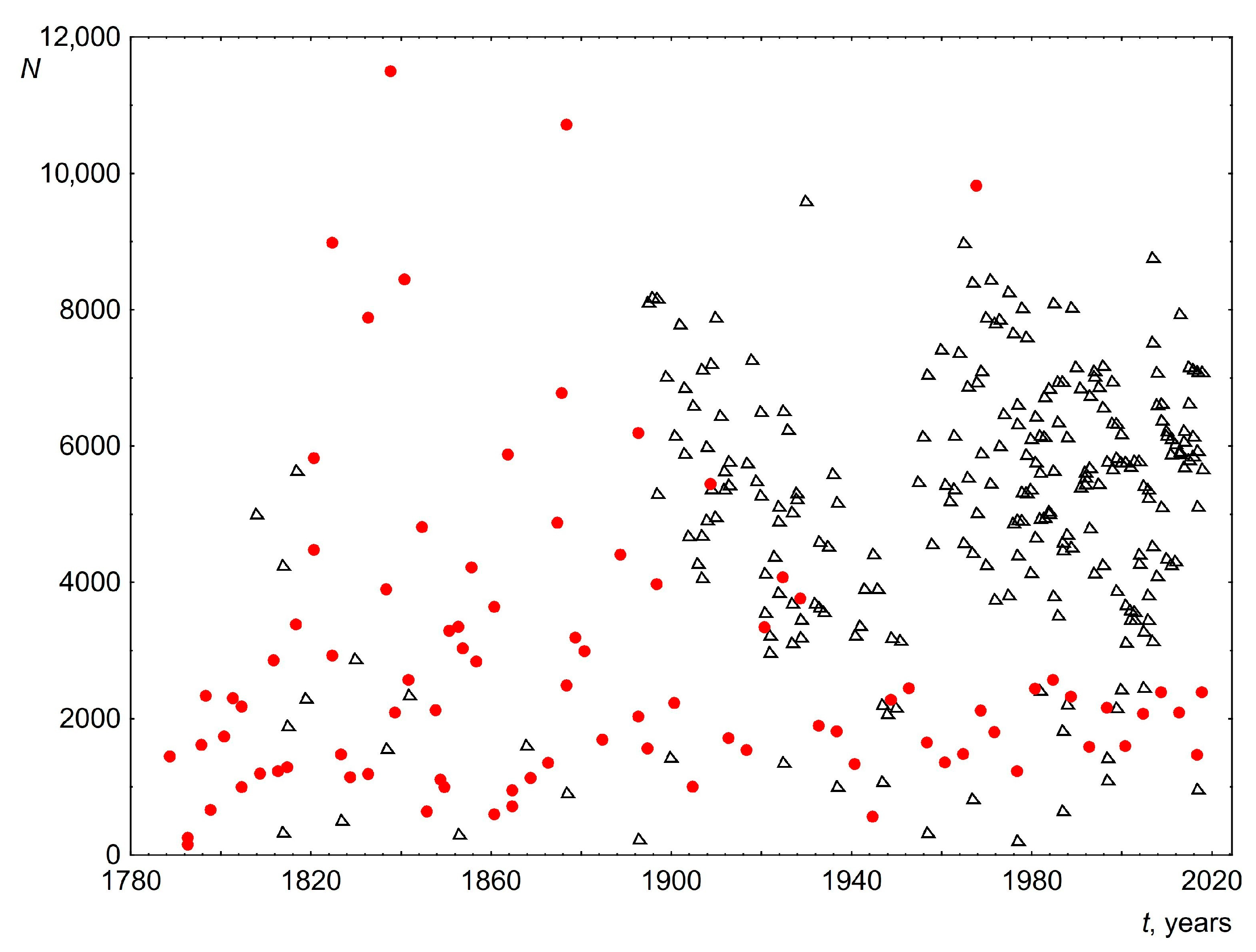
4. Change in Word Length over Time

A number of quantities were calculated to analyze the possible change in word length over time. They are listed below:

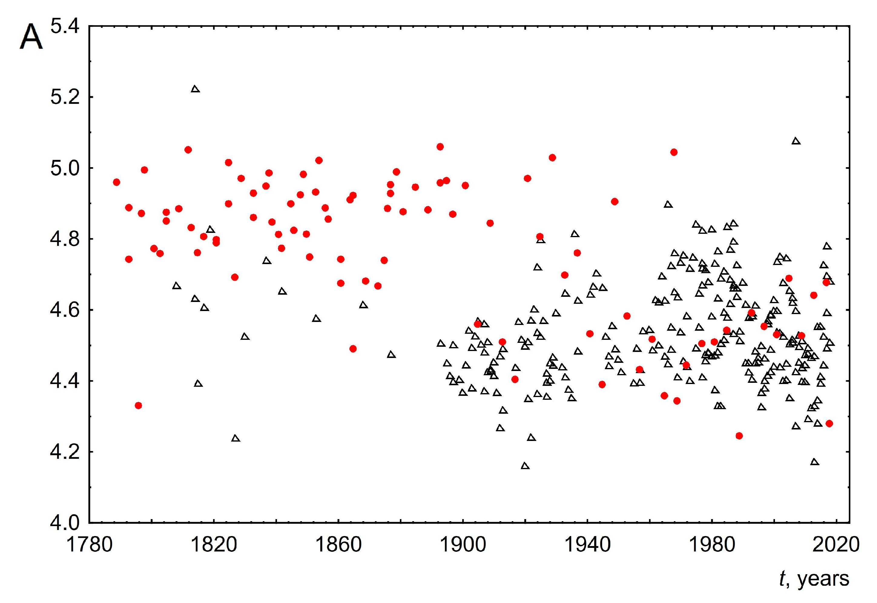
• The average word length. To calculate this parameter, the total number of letters in a speech is divided by the number of words. The change in this parameter over time is shown in Figure 5. As can be seen from the graph, the average word length for UK speeches has remained almost unchanged over two hundred years and is about 4.5. For USA speeches, the result is more complicated. So, from 1789 to about 1950, the average length of words practically did not change and was about 4.9. However, then there is a small stepwise change in the average word length to 4.5. As a result, from 1950 to the present, the average length of words for both the USA and the UK is the same. Within quantitative linguistics it is impossible to understand the reasons for such behavior. However, based on historical facts, we will put forward the following hypotheses to explain this behavior. (1) Initially, USA presidents made speeches only before Congress; other citizens became acquainted with their speeches through newspapers. Such speeches only began to be fully broadcasted on radio and television after the Second World War. This may have led to the observed decrease in average word length. (2) The unchanged average word length for the UK can be explained, apparently, by the fact that the speeches were made before members of Parliament, a rather conservative representative body with strong centuries-old traditions. Adherence to tradition is a quality that is often used to describe British society as a whole. This is illustrated by the result obtained in the work about the unchanged average length of words of parliamentarians over more than two hundred years. (3) It was after the Second World War that a special relationship emerged between the USA and the UK. The term “special relationship” publicly emerged in Winston Churchill’s “Iron Curtain” speech of 1946. The special relationship is a term that is often used to describe the close historic, political, military, economic and cultural relations between USA and UK political leaders and elites. This could be the reason that the vocabulary of USA and UK politicians became very close after the war and, as a consequence, the average length of words is the same.

2.

The median of the word length distribution for all speeches was found to be four and did not change over time.

3.

The maximum word length of speeches delivered over 200 years also did not change and was in the range from 14 to 16. Examples of these most common words for the USA: accountability, administration, constitutional, accomplishment, irresponsibility. For the UK, these words are responsibility, congratulation, disestablishment, apprenticeship, discrimination, internationalism.

4.

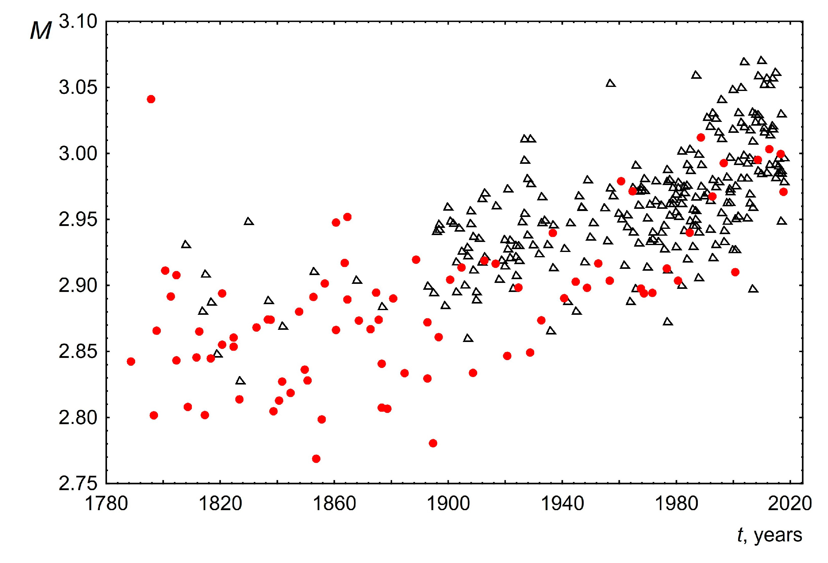
The mode for each of the speeches was calculated based on the averaging of the three most probable word lengths. The averaging was performed taking into account the probabilities of occurrence of these three values in the text. This was performed to make this parameter more sensitive to the shape and width of the length distribution near the maximum. The change in the mode of the word length distribution over time is shown in Figure 6. As can be seen, the mode of word lengths of public speeches for both the USA and the UK increases slightly over 200 years from 2.85 to 3.02. This change is approximately linear with a slope of 0.0005± 0.0002 for the USA and 0.0006 ± 0.0001 for the UK.

5.

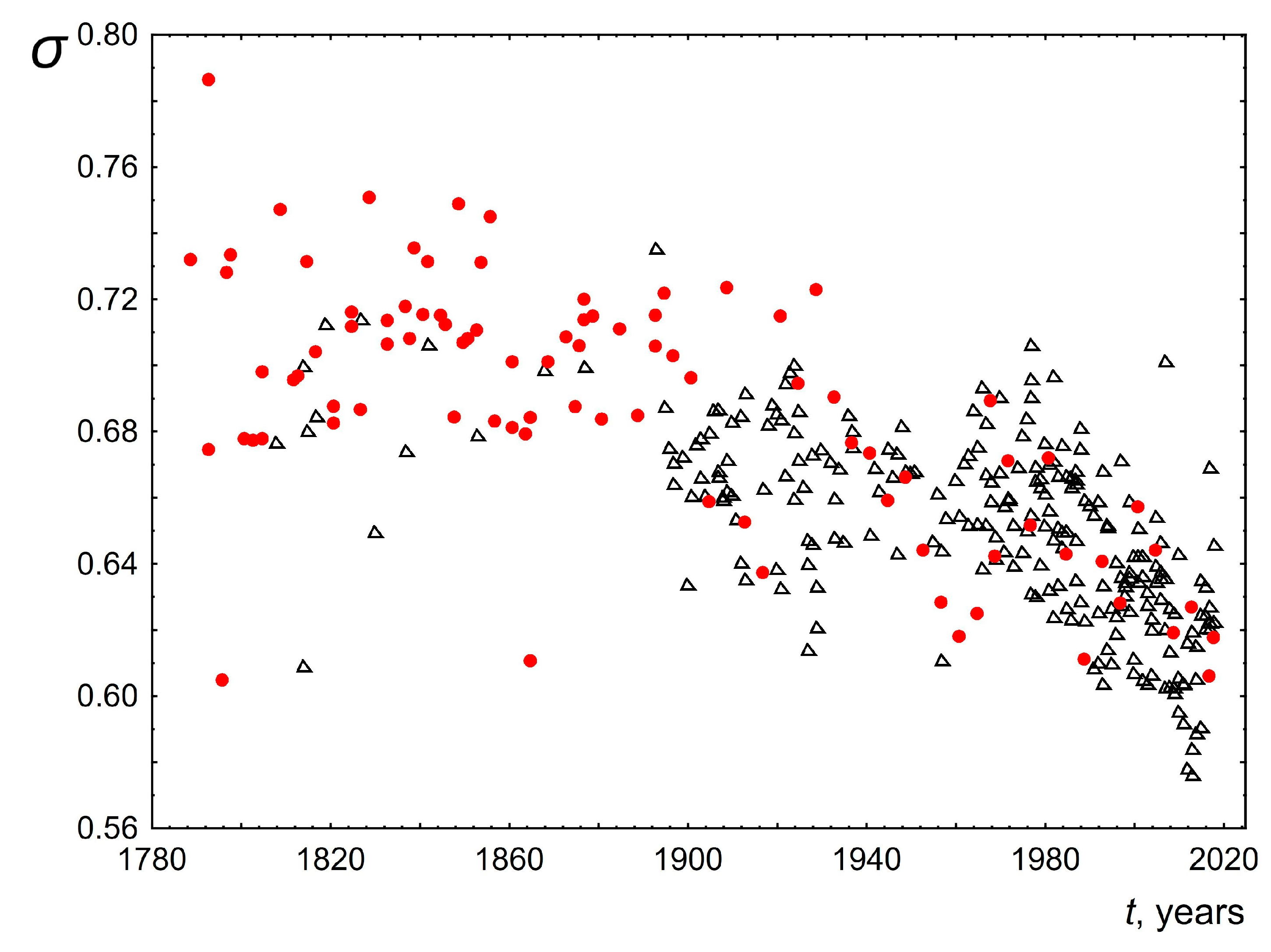
Figure 7 and Figure 8 show the dependence of the parameters of the lognormal distribution µ, σ on time. As can be seen, µ does not depend on time, remaining approximately equal to 1.25. At the same time, the parameter σ slightly decreases over 200 years from 0.74 to 0.62. These results are consistent with the results presented in Figure 5 and Figure 6. Indeed, as we know, the mean value for a lognormal distribution is related to µ, σ as $\mathrm{e}\mathrm{x}\mathrm{p}(\mu +{\sigma }^2/2)$. As a consequence, when µ is constant and σ decreases the mean value will decrease. On the other hand, since the mode is related to µ, σ as $\mathrm{e}\mathrm{x}\mathrm{p}(\mu -{\sigma }^2)$, then when µ remains constant and σ decreases, the mode should increase. The above agreement in the behavior of the parameters of the lognormal distribution µ, σ (Figure 7 and Figure 8) with the results based on the analysis of directly empirical histograms (Figure 5 and Figure 6) provides an additional argument for the applicability of the lognormal distribution to describe the distribution of word lengths.

The change in the probability density of the lognormal distribution with time is presented in Figure 9. It can be seen that this change is very insignificant over two hundred years.

5. Conclusions

This paper shows that the lognormal distribution is better applicable to describe the distribution of word lengths in the texts of public speeches by politicians. This is significantly different from the result obtained for the sentence length distribution, in which the Weibull distribution is preferred [9]. As a consequence, we can conclude that the principle of least effort does not have a significant impact on the length of words used by politicians. As is known, an important reason for the appearance of a lognormal distribution is the presence of a multiplicative random process that determines the random variable [27]. In our case, such a random variable is the length of the word.

It is found that word length in public speeches of USA and UK politicians has remained almost unchanged over the last two hundred years. There has been a very slight decrease in the average value for the USA and a slight increase in the most probable word length (mode). This result differs significantly from the results obtained previously for sentence lengths, the lengths of which decreased significantly over time [9]. The result obtained for words is quite surprising. Indeed, for such a long period of time, many very significant historical events have occurred for humanity, new techniques and technologies have appeared and improved explosively and enormous cultural and social changes have taken place in society. All this inevitably led to the emergence of new words and should have affected the frequency of use of existing words. However, as statistical analysis has shown, the length of words used has not changed much. Apparently, the length of words is statistically a very conservative parameter, which turns out to be insensitive to the above changes. These changes affect words in different ways, which do not affect their average length.

The results obtained in this paper question not only the applicability of the principle of least effort, but indicate a possible limitation of the Menzerath–Altmann, Zipf and brevity laws for analyzing word lengths in public speaking. We base this conclusion on the following logic. (1) As discussed above (see also [9]) the feasibility of the principle of least effort should lead to a Weibull distribution for word lengths and to a decrease in average word lengths over time. However, neither one nor the other was found. (2) Since it was previously discovered in [9] that the length of sentences decreases significantly, then, based on the constancy of the length of words over time obtained for the same speeches, it follows that the Menzerath–Altmann law is inapplicable for the sentence/word pair in the speeches of politicians. (3) Since the consequence of the Zipf and brevity laws is a power–law dependence of the frequency of words on their length, the established lognormal distribution for word lengths shows the limitations of these laws, at least when considering all word lengths, including the shortest ones.

There are quite a lot of laws in quantitative linguistics, only a small part of which we critically discuss in this article. These laws (statements) do not have the same degree of generality and universal acceptance as, for example, can be seen in physics. If we use the terminology of physics, then these statements in quantitative linguistics can be called working hypotheses rather than laws. These working hypotheses need clarification and adjustment. Thanks to research like the present one, this work of turning working hypotheses into laws is taking place.

It is important to emphasize in conclusion, following [4], that word length is an essential property of a word; from the point of view of quantitative linguistics, word length with its relationships with other linguistic structures and levels provides information that is an important part of the general theory of language.

References

- Altmann, G. Prolegomena to Menzerath’s law. Glottometrika 1980, 2, 1–10. [Google Scholar]
- Zipf, G.K. Human Behavior and the Principle of Least Effort: An Introduction to Human Ecology; Addison-Wesley Publishing: Cambridge, UK, 1949. [Google Scholar]
- Popescu, I.; Naumann, S.; Kelih, E.; Rovenchak, A.; Overbeck, A.; Sanada, H.; Smith, R.D.; Čech, R.; Mohanty, P.; Wilson, A. Word length: Aspects and languages. Issues Quant. Linguist. 2013, 3, 224–281. [Google Scholar]
- Grzybek, P. (Ed.) Contributions to the Science of Text and Language: Word Length Studies and Related Issues; Springer Science & Business Media: Dordrecht, The Netherlands, 2006; Volume 31. [Google Scholar]
- Rottmann, O.A. On Word Length in German and Polish. Glottometrics 2018, 42, 13–20. [Google Scholar]
- Vieira, D.S.; Picoli, S.; Mendes, R.S. Robustness of sentence length measures in written texts. Phys. A Stat. Mech. Its Appl. 2018, 506, 749–754. [Google Scholar] [CrossRef]
- Milička, J. Average Word Length from the Diachronic Perspective: The Case of Arabic. Linguist. Front. 2018, 1, 81–89. [Google Scholar] [CrossRef]
- Liberman, M. Real Trends in Word and Sentence Length. 2011. Available online: http://languagelog.ldc.upenn.edu/nll (accessed on 25 December 2023).
- Tsizhmovska, N.L.; Martyushev, L.M. Principle of least effort and sentence length in public speaking. Entropy 2021, 23, 1023. [Google Scholar] [CrossRef]
- Tucker, E.C.; Capps, C.J.; Shamir, L. A data science approach to 138 years of congressional speeches. Heliyon 2020, 6, e04417. [Google Scholar] [CrossRef] [PubMed]
- Bochkarev, V.V.; Shevlyakova, A.V.; Solovyev, V.D. The average word length dynamics as an indicator of cultural changes in society. Soc. Evol. Hist. 2015, 14, 153–175. [Google Scholar]
- Lenard, D.B. Gender differences in the length of words and sentences on the corpus of congressional speeches. Imp. J. Interdiscip. Res. 2016, 2, 1417–1424. [Google Scholar]
- Corral, Á.; Serra, I. The brevity law as a scaling law, and a possible origin of zipf’s law for word frequencies. Entropy 2020, 22, 224. [Google Scholar] [CrossRef] [PubMed]
- Chen, H.; Liu, H. A diachronic study of Chinese word length distribution. Glottometrics 2014, 29, 81–94. [Google Scholar]
- Sigurd, B.; Eeg-Olofsson, M.; Van de Weijer, J. Word length, sentence length and frequency—Zipf revisited. Stud. Linguist. 2004, 58, 37–52. [Google Scholar] [CrossRef]
- Grzybek, P. Word Length. In The Oxford Handbook of the Word; Taylor, J.R., Ed.; Oxford Academic: Oxford, UK, 2015. [Google Scholar]
- Torre, I.G.; Luque, B.; Lacasa, L.; Kello, C.T.; Hernández-Fernández, A. On the physical origin of linguistic laws and lognormality in speech. R. Soc. Open Sci. 2019, 6, 191023. [Google Scholar] [CrossRef] [PubMed]
- Rosen, K.M. Analysis of speech segment duration with the lognormal distribution: A basis for unification and comparison. J. Phon. 2005, 33, 411–426. [Google Scholar] [CrossRef]
- Kosmidis, K.; Kalampokis, A.; Argyrakis, P. Language time series analysis. Phys. A Stat. Mech. Its Appl. 2006, 370, 808–816. [Google Scholar] [CrossRef]
- University of Virginia. Famous Presidential Speeches of the United States. Available online: https://millercenter.org/the-presidency/presidential-speeches (accessed on 1 January 2022).
- Inaugural Addresses of the Presidents of the United States. Available online: https://www.bartleby.com/124/ (accessed on 25 July 2021).
- British Political Speech; Swansea University: Swansea, UK. Available online: http://britishpoliticalspeech.org/index.htm (accessed on 25 July 2021).
- UK Parliament 2023. Hansard. Available online: https://hansard.parliament.uk/ (accessed on 1 January 2022).
- Montemurro, M.A.; Pury, P.A. Long-range fractal correlations in literary corpora. Fractals 2002, 10, 451–461. [Google Scholar] [CrossRef]
- Grzybek, P. History and Methodology of Word Length Studies: The State of the Art; Springer: Dordrecht, The Netherlands, 2007; pp. 15–90. [Google Scholar]
- Tsizhmovska, N.L. Word Length in Public Speaking; Ural Federal University: Yekaterinburg, Russia, 2023; Available online: https://github.com/Kototiapa/Word-Length-in-Public-Speaking (accessed on 1 January 2022).
- Sobkowicz, P.; Thelwall, M.; Buckley, K.; Paltoglou, G.; Sobkowicz, A. Lognormal distributions of user post lengths in Internet discussions—A consequence of the Weber-Fechner law? EPJ Data Sci. 2013, 2, 1–20. [Google Scholar] [CrossRef]