
A Fast Algorithm for Estimating Two-Dimensional Sample Entropy Based on an Upper Confidence Bound and Monte Carlo Sampling

Abstract
1. Introduction
2. Fast Algorithms for Estimating Two-Dimensional Sample Entropy
2.1. Groundwork of Two-Dimensional Sample Entropy
| Algorithm 1 Two-dimensional sample entropy |
|
2.2. A Monte Carlo-Based Algorithm for Estimating Two-Dimensional Sample Entropy
| Algorithm 2 Two-dimensional Monte Carlo sample entropy (MCSampEn2D) |
|
2.3. Monte Carlo Sample Entropy Based on the UCB Strategy
| Algorithm 3 Monte Carlo sample entropy based on UCB strategy |
Sample numbers and epoch numbers .
|
3. Experiments
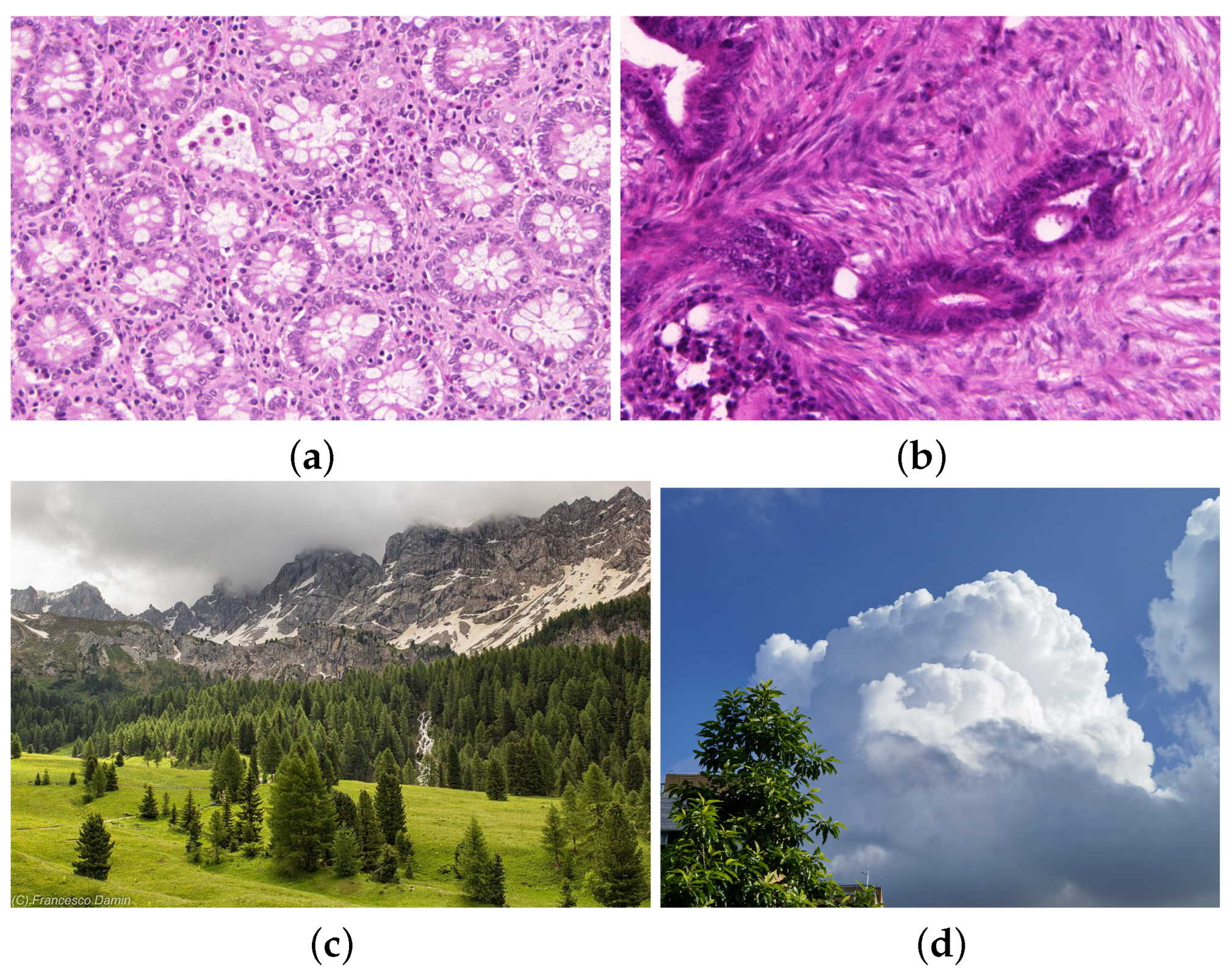
3.1. Datasets
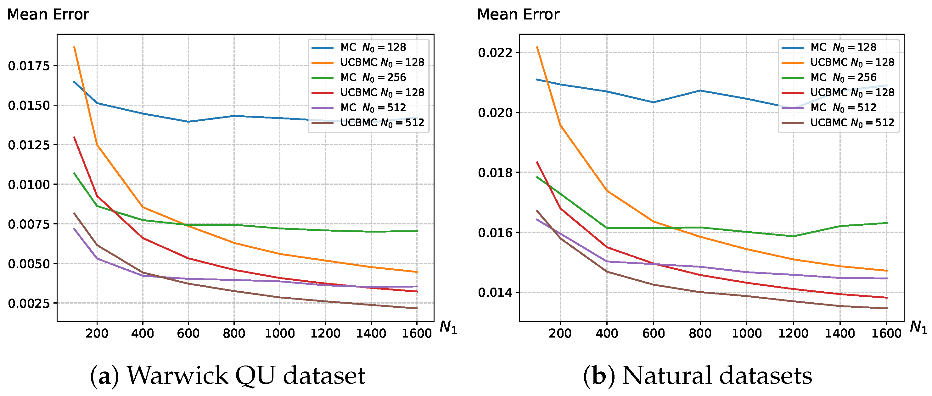
3.2. Main Results
4. Discussion
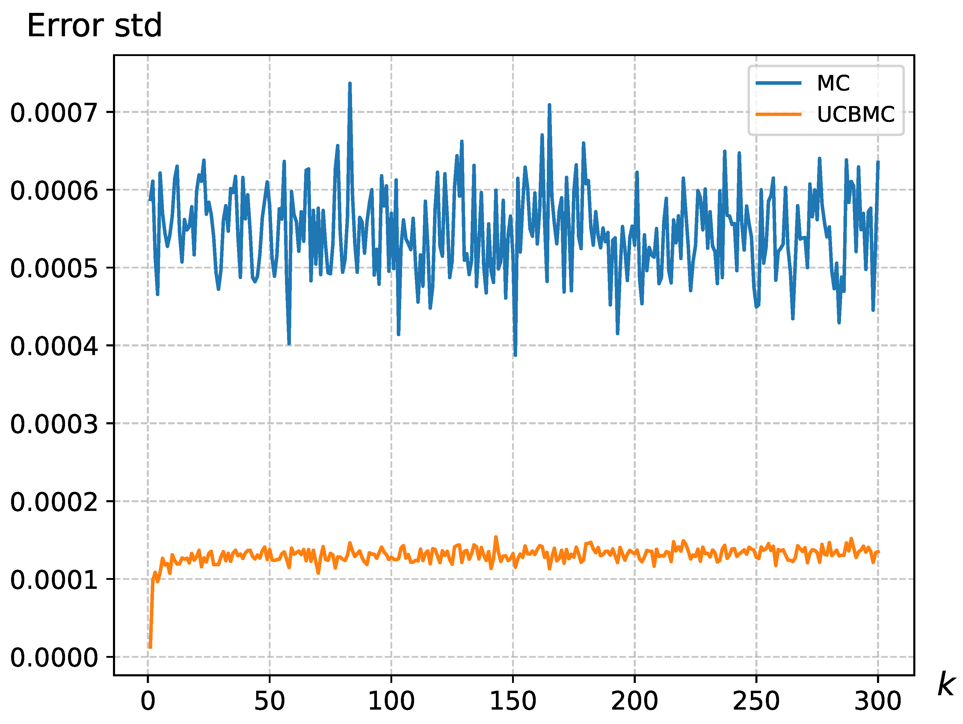
4.1. Analysis of the UCB Strategy
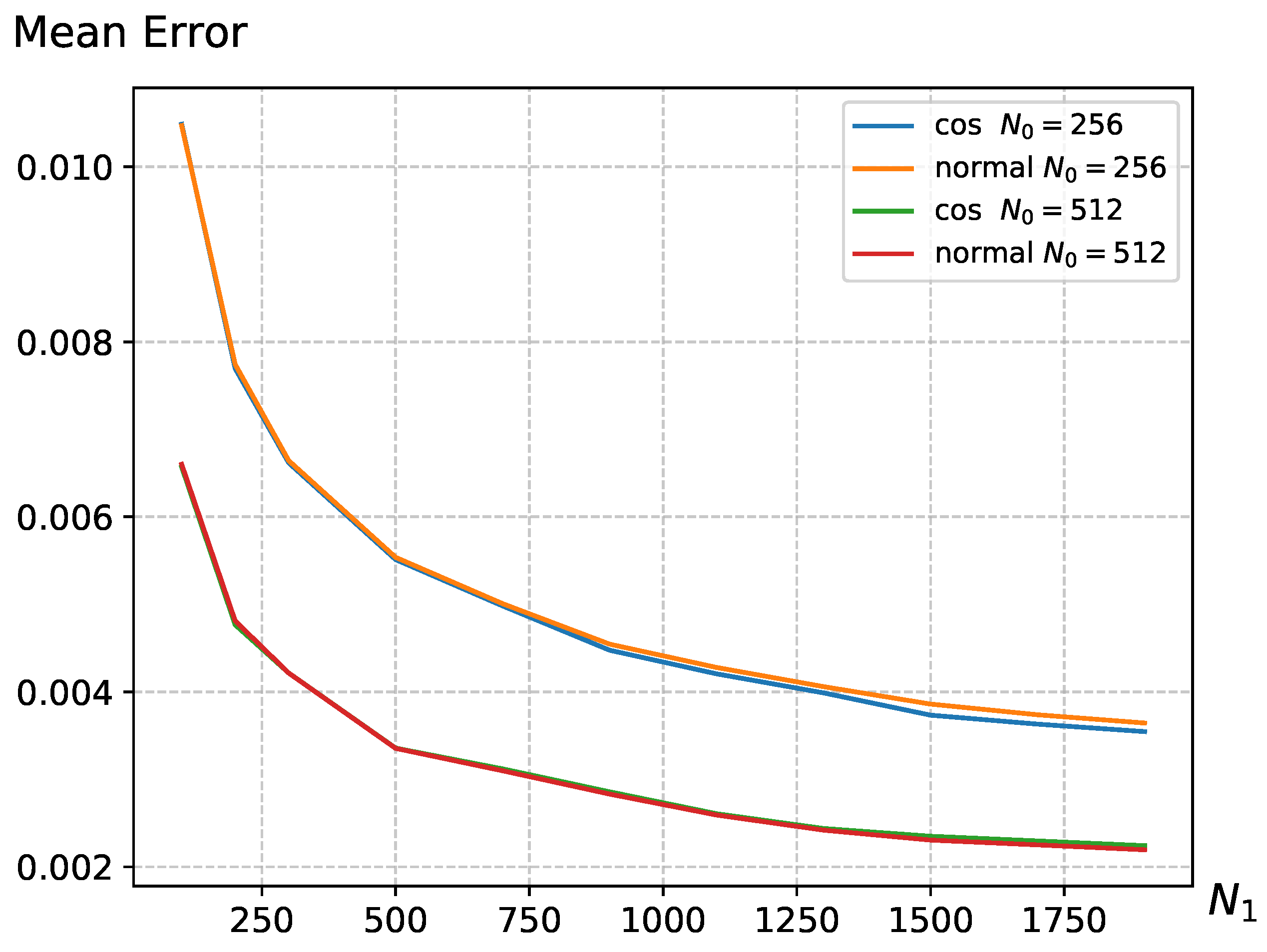
4.2. The Impact of Parameters on the UCB Strategy
4.3. The Application of Sample Entropy in Medical Image Dataset
5. Conclusions
Author Contributions
Funding
Data Availability Statement
Conflicts of Interest
References
- Shannon, C.E. A Mathematical Theory of Communication. Assoc. Comput. Mach. 2001, 5, 1559–1662. [Google Scholar] [CrossRef]
- Richman, J.S.; Moorman, J.R. Physiological time-series analysis using approximate entropy and sample entropy. Am. J. Physiol. Heart Circ. Physiol. 2000, 278, H2039–H2049. [Google Scholar] [CrossRef] [PubMed]
- Pincus, S.M. Approximate entropy as a measure of system complexity. Proc. Natl. Acad. Sci. USA 1991, 88, 2297–2301. [Google Scholar] [CrossRef] [PubMed]
- Tomčala, J. New fast ApEn and SampEn entropy algorithms implementation and their application to supercomputer power consumption. Entropy 2020, 22, 863. [Google Scholar] [CrossRef] [PubMed]
- Rostaghi, M.; Azami, H. Dispersion entropy: A measure for time-series analysis. IEEE Signal Process. Lett. 2016, 23, 610–614. [Google Scholar] [CrossRef]
- Li, Y.; Li, G.; Yang, Y.; Liang, X.; Xu, M. A fault diagnosis scheme for planetary gearboxes using adaptive multi-scale morphology filter and modified hierarchical permutation entropy. Mech. Syst. Signal Proc. 2017, 105, 319–337. [Google Scholar] [CrossRef]
- Yang, C.; Jia, M. Hierarchical multiscale permutation entropy-based feature extraction and fuzzy support tensor machine with pinball loss for bearing fault identification. Mech. Syst. Signal Proc. 2021, 149, 107182. [Google Scholar] [CrossRef]
- Li, W.; Shen, X.; Yaan, L. A comparative study of multiscale sample entropy and hierarchical entropy and its application in feature extraction for ship-radiated noise. Entropy 2019, 21, 793. [Google Scholar] [CrossRef] [PubMed]
- Aboy, M.; Cuesta-Frau, D.; Austin, D.; Mico-Tormos, P. Characterization of sample entropy in the context of biomedical signal analysis. In Proceedings of the 2007 29th Annual International Conference of the IEEE Engineering in Medicine and Biology Society, Lyon, France, 22–26 August 2007; pp. 5942–5945. [Google Scholar]
- Jiang, Y.; Mao, D.; Xu, Y. A fast algorithm for computing sample entropy. Adv. Adapt. Data Anal. 2011, 3, 167–186. [Google Scholar] [CrossRef]
- Mao, D. Biological Time Series Classification via Reproducing Kernels and Sample Entropy. Ph.D. Thesis, Syracuse University, Syracuse, NY, USA, 2008. [Google Scholar]
- Schreiber, T.; Grassberger, P. A simple noise-reduction method for real data. Phys. Lett. A 1991, 160, 411–418. [Google Scholar] [CrossRef]
- Theiler, J. Efficient algorithm for estimating the correlation dimension from a set of discrete points. Phys. Rev. A Gen. Phys. 1987, 36, 4456–4462. [Google Scholar] [CrossRef] [PubMed]
- Manis, G. Fast computation of approximate entropy. Comput. Meth. Prog. Bio. 2008, 91, 48–54. [Google Scholar] [CrossRef] [PubMed]
- Manis, G.; Aktaruzzaman, M.; Sassi, R. Low computational cost for sample entropy. Entropy 2018, 20, 61. [Google Scholar] [CrossRef] [PubMed]
- Wang, Y.H.; Chen, I.Y.; Chiueh, H.; Liang, S.F. A Low-Cost Implementation of Sample Entropy in Wearable Embedded Systems: An Example of Online Analysis for Sleep EEG. IEEE Trans. Instrum. Meas. 2021, 70, 9312616. [Google Scholar] [CrossRef]
- Liu, W.; Jiang, Y.; Xu, Y. A Super Fast Algorithm for Estimating Sample Entropy. Entropy 2022, 24, 524. [Google Scholar] [CrossRef] [PubMed]
- Garivier, A.; Moulines, E. On upper-confidence bound policies for switching bandit problems. In Proceedings of the International Conference on Algorithmic Learning Theory, Espoo, Finland, 5–7 October 2011; pp. 174–188. [Google Scholar]
- Anderson, T. Towards a theory of online learning. Theory Pract. Online Learn. 2004, 2, 109–119. [Google Scholar]
- Silva, L.E.V.; Senra Filho, A.C.S.; Fazan, V.P.S.; Felipe, J.C.; Murta, L.O., Jr. Two-dimensional sample entropy: Assessing image texture through irregularity. Biomed. Phys. Eng. Express 2016, 2, 045002. [Google Scholar] [CrossRef]
- da Silva, L.E.V.; da Silva Senra Filho, A.C.; Fazan, V.P.S.; Felipe, J.C.; Murta, L.O., Jr. Two-dimensional sample entropy analysis of rat sural nerve aging. In Proceedings of the 2014 36th Annual International Conference of the IEEE Engineering in Medicine and Biology Society, Chicago, IL, USA, 26–30 August 2014; pp. 3345–3348. [Google Scholar]
- Audibert, J.-Y.; Munos, R.; Szepesvári, C. Exploration–exploitation tradeoff using variance estimates in multi-armed bandits. Theor. Comput. Sci. 2009, 410, 1876–1902. [Google Scholar] [CrossRef]
- Zhou, D.; Li, L.; Gu, Q. Neural contextual bandits with ucb-based exploration. In Proceedings of the International Conference on Machine Learning, Virtual, 13–18 July 2020; pp. 11492–11502. [Google Scholar]
- Gupta, N.; Granmo, O.-C.; Agrawala, A. Thompson sampling for dynamic multi-armed bandits. In Proceedings of the 2011 10th International Conference on Machine Learning and Applications and Workshops, Honolulu, HI, USA, 18–21 December 2011; Volume 1, pp. 484–489. [Google Scholar]
- Cheung, W.C.; Simchi-Levi, D.; Zhu, R. Learning to optimize under non-stationarity. In Proceedings of the 22nd International Conference on Artificial Intelligence and Statistics, Naha, Japan, 16–18 April 2019; pp. 1079–1087. [Google Scholar]
- Xu, M.; Qin, T.; Liu, T.-Y. Estimation bias in multi-armed bandit algorithms for search advertising. In Proceedings of the 26th International Conference on Neural Information Processing Systems, Lake Tahoe, NV, USA, 5–10 December 2013. [Google Scholar]
- Sarwinda, D.; Paradisa, R.H.; Bustamam, A.; Anggia, P. Deep learning in image classification using residual network (ResNet) variants for detection of colorectal cancer. Procedia Comput. Sci. 2021, 179, 423–431. [Google Scholar] [CrossRef]


| Method | / | Mean Error (Proportion) | Mean Time (s) |
|---|---|---|---|
| SampEn2D | / | / | 402.98 |
| 128/1300 | 4.91 | ||
| MCSampEn2D | 256/1100 | 4.29 | |
| 512/900 | 4.87 | ||
| 128/1300 | 4.91 | ||
| UCBMCSampEn2D | 256/1100 | 4.29 | |
| 512/900 | 4.87 |
| SampEn2D | MCSampEn2D | UCBMCSampEn2D | |
|---|---|---|---|
| time(s) | 161,322 | 1.5816 | 0.9057 |
| error | / |
| SampEn2D | MCSampEn2D | UCBMCSampEn2D | |
|---|---|---|---|
| time (s) | 230.546 | 1.4046 | 0.9773 |
| error | / |
| Image Name | UCBMCSampEn2D | Benign or Malignant |
|---|---|---|
| testB_1 | 0.317812 | Benign |
| train_15 | 0.529283 | Benign |
| train_47 | 0.672241 | Benign |
| testA_17 | 0.762295 | Benign |
| testA_24 | 1.06252 | Benign |
| testA_57 | 2.37266 | Malignant |
| testA_59 | 2.1973 | Malignant |
| testA_8 | 2.36954 | Malignant |
| testA_19 | 2.10283 | Malignant |
| testB_7 | 2.07255 | Malignant |
Disclaimer/Publisher’s Note: The statements, opinions and data contained in all publications are solely those of the individual author(s) and contributor(s) and not of MDPI and/or the editor(s). MDPI and/or the editor(s) disclaim responsibility for any injury to people or property resulting from any ideas, methods, instructions or products referred to in the content. |
© 2024 by the authors. Licensee MDPI, Basel, Switzerland. This article is an open access article distributed under the terms and conditions of the Creative Commons Attribution (CC BY) license (https://creativecommons.org/licenses/by/4.0/).
Share and Cite
Zhou, Z.; Jiang, Y.; Liu, W.; Wu, R.; Li, Z.; Guan, W. A Fast Algorithm for Estimating Two-Dimensional Sample Entropy Based on an Upper Confidence Bound and Monte Carlo Sampling. Entropy 2024, 26, 155. https://doi.org/10.3390/e26020155
Zhou Z, Jiang Y, Liu W, Wu R, Li Z, Guan W. A Fast Algorithm for Estimating Two-Dimensional Sample Entropy Based on an Upper Confidence Bound and Monte Carlo Sampling. Entropy. 2024; 26(2):155. https://doi.org/10.3390/e26020155
Chicago/Turabian StyleZhou, Zeheng, Ying Jiang, Weifeng Liu, Ruifan Wu, Zerong Li, and Wenchao Guan. 2024. "A Fast Algorithm for Estimating Two-Dimensional Sample Entropy Based on an Upper Confidence Bound and Monte Carlo Sampling" Entropy 26, no. 2: 155. https://doi.org/10.3390/e26020155
APA StyleZhou, Z., Jiang, Y., Liu, W., Wu, R., Li, Z., & Guan, W. (2024). A Fast Algorithm for Estimating Two-Dimensional Sample Entropy Based on an Upper Confidence Bound and Monte Carlo Sampling. Entropy, 26(2), 155. https://doi.org/10.3390/e26020155