
Symplectic Bregman Divergences


Sony Computer Science Laboratories Inc., Tokyo 141-0022, Japan
Entropy 2024, 26(12), 1101; https://doi.org/10.3390/e26121101
Submission received: 26 August 2024
/
Revised: 5 December 2024
/
Accepted: 15 December 2024
/
Published: 16 December 2024
(This article belongs to the Special Issue Information Geometry for Data Analysis)
Abstract
We present a generalization of Bregman divergences in finite-dimensional symplectic vector spaces that we term symplectic Bregman divergences. Symplectic Bregman divergences are derived from a symplectic generalization of the Fenchel–Young inequality which relies on the notion of symplectic subdifferentials. The symplectic Fenchel–Young inequality is obtained using the symplectic Fenchel transform which is defined with respect to the symplectic form. Since symplectic forms can be built generically from pairings of dual systems, we obtain a generalization of Bregman divergences in dual systems obtained by equivalent symplectic Bregman divergences. In particular, when the symplectic form is derived from an inner product, we show that the corresponding symplectic Bregman divergences amount to ordinary Bregman divergences with respect to composite inner products. Some potential applications of symplectic divergences in geometric mechanics, information geometry, and learning dynamics in machine learning are touched upon.
1. Introduction
Symplectic geometry [1,2,3] was historically pioneered by Lagrange around 1808–1810 [4,5,6] where the motions and dynamics (evolution curves) of a finite set of m point mass particles in a time interval T are analyzed in the phase space by a 1D curve , where ’s denote the point locations at time t and ’s encode the momentum, i.e., with . See Figure 1. (Notice that Joseph-Louis Lagrange (1736–1813) was 72 years old in 1808, and is famous for his treatise on analytic mechanics [7,8] published first in french in 1788 when he was 52 years old).
The Hamiltonian coupled equations [9] governing the system motion are written in the phase space as follows:
where is the Hamiltonian describing the system. Lagrange originally started a new kind of calculus, “symplectic calculus”. Symplectic geometry can be thought as the first discovered non-Euclidean geometric structure since hyperbolic geometry is usually considered to be first studied by Lobachevsky and Bolyai around 1820–1930. We refer to the paper entitled “The symplectization of science” [10] for an outreach article on symplectic geometry.
The adverb “symplectic” stems from Greek: It means “braided together” to convey the interactions of point mass particle positions with their momenta. Its use in mathematics originated in the work of Hermann Weyl (see §6 on symplectic groups in [11]). Another synonym adverb of symplectic is “complex” which has been used to describe braided numbers z of . Complex has its etymological root in Latin. In differential geometry, symplectic structures are closely related to (almost) complex structures on vector spaces and smooth manifolds [2].
In physics, symplectic geometry is not only at the core of classical mechanics (i.e., conservative reversible mechanics) and quantum mechanics [12], but has also recently been used to model and study dynamics of systems exhibiting dissipative terms [13,14] which are irreversible. As a pure geometry, symplectic geometry can be studied on its own by mathematicians, and gave birth to the field of symplectic topology [15]. Thus, symplectic geometry can be fruitfully applied to various areas beyond its original domain of geometric mechanics. For example, symplectic geometry has been considered in machine learning for accelerating numerical optimization methods based on symplectic integrators [16] and in physics-informed neural networks [17,18] (PINNs).
In this paper, we define symplectic Bregman divergences (Definition 5) which recover as special cases Bregman divergences [19] defined with respect to composite inner products. A Bregman divergence induced by a strictly convex and differentiable (potential) function F (called the Bregman generator) between and of X is defined in [19] (1967) by
where is an inner product on X. Let denote the set of functions which are lower semi-continuous convex with non-empty effective domains. The convex conjugate obtained by the Legendre–Fenchel transform yields a dual Bregman divergence when the function is of Legendre type [20,21]:
such that with
This paper introduces and extends the work of Buliga and Saxcé [13,14] which is motivated by geometric irreversible mechanics. To contrast with [13,14], this expository paper is targeted to an audience familiar with Bregman divergences [19] in machine learning and information geometry [22] but does not assume any prior knowledge in geometric mechanics. Furthermore, we consider only finite-dimensional spaces in this study.
The paper is organized as follows: In Section 2, we define symplectic vector spaces and explain the representation of symplectic forms using dual pairings. We then define the symplectic Fenchel transform and the symplectic Fenchel–Young inequality in Section 3. The definitions of symplectic Fenchel–Young divergences (Definition 4) and symplectic Bregman divergences (Definition 5) are reported in Section 4. In particular, we show how to recover Bregman divergences with respect to composite inner products as special cases in Section 5 (Property 1). In general, symplectic Bregman divergences allow one to define Bregman divergences in dual systems equipped with pairing products. Finally, we recall the role of Bregman divergences in dually flat manifolds of information geometry in Section 6, and motivate the introduction of symplectic Bregman divergences in geometric mechanics (e.g., symplectic BEN principle of [13,14]) and learning dynamics in machine learning.
2. Dual Systems, Linear Symplectic Forms, and Symplectomorphisms
2.1. Symplectic Forms Derived from Dual Systems
We begin with two definitions:
Definition 1
(Dual system). Let X and Y be finite m-dimensional vector spaces [23] equipped with a pairing product , i.e., a bilinear map:
such that all continuous linear functionals on X and Y are expressed as and , respectively. The triplet forms a dual system.
(Notice that when the type of X is different from the type of Y then the bilinear map cannot be symmetric).
Definition 2
(Symplectic vector space). A symplectic vector space is a vector space equipped with a map [24] which is
- 1.
- bilinear: , we have
- 2.
- skew-symmetric (or alternating): , and
- 3.
- non-degenerate: if for a , we have for all then we have .
Notice that skew-symmetry implies that for all since and hence . The map is called a linear symplectic form [24,25].
We define the symplectic form induced by the pairing product of a dual system as follows:
where and belong to .
Let us report several examples of linear symplectic forms:
- Let be a finite n-dimensional vector space with the dual space of linear functionals (space of covectors l). The natural pairing of a vector with a covector is an example of dual product. (We use the superscript index for indicating components of contravariant vectors and subscript index for specifying components of covariant vectors [9]). We define the symplectic form induced by the natural pairing of vectors with covectors as follows:where and belong to .
- Consider an inner product space of dimension n. The product space of even dimension n can be equipped with the following map induced by the inner product:where and .
For example, let and . Then . This symplectic form can be interpreted as the determinant of the matrix which corresponds geometrically to the signed orientation of the parallelogram defined by the vectors and . See Figure 2. (This example indicates the link with integration of 2D manifolds equipped with fields of symplectic forms smoothly varying called differential 2-forms [9]).
In a finite-dimensional vector space, we can express the inner product as for a symmetric positive-definite matrix . Let be the Cholesky decomposition of Q. Then we have
where I is the identity matrix and is the Euclidean inner product. Thus the form induced by can be expressed using linear algebra as
where is a skew-symmetric matrix: . More generally, we may consider skew-symmetric matrices of the form to define the symplectic form induced by the inner product .
2.2. Linear Symplectomorphisms and the Groups of Symplectic Matrices
A symplectic form can be expressed as a matrix such that where are the basis vectors, and .
The Darboux basis [2] of the canonical form of is such that and where denotes the Kronecker delta function. is the symplectic matrix corresponding to the canonical form of .
A transformation is called a linear symplectomorphism when (i.e., ), i.e., when where T be the matrix representation of t. In particular t is a linear symplectomorphism with respect to when . Any symplectic vector space of dimension is symplectomorphic to the canonical symplectic space .
Linear symplectomorphisms can be represented by symplectic matrices of the symplectic group [11,26] :
Transpose and inverse of symplectic matrices are symplectic matrices. The inverse of a symplectic matrix T is given by
Symplectic matrices of have unit determinant (), and in the particular case of , corresponds precisely to the set of matrices with unit determinant. Thus rotation matrices of which have unit determinant for a subgroup of .
Sesquilinear symplectic forms can also be defined on complex linear spaces [27].
3. Symplectic Fenchel Transform, Symplectic Subdifferentials, and Symplectic Fenchel–Young (in)Equality
Let be a convex lower semi-continuous (lsc) function called a potential function.
Definition 3
(Symplectic Fenchel conjugate). The symplectic Fenchel conjugate is defined by
Notice that since is skew-symmetric, the order of the arguments in is important: The symplectic Fenchel transform optimizes with respect to the second argument of .
The symplectic subdifferential of F at z is defined by
The differential operator is a set-valued operator: , where is the set of potential functions. An element of the symplectic subdifferential of F at z is called a symplectic subgradient.
Remark 1.
Moreau generalized the Fenchel conjugate using a cost function [28]. In particular, the duality induced by logarithmic cost function was studied in [29], and lead to a generalization of Bregman divergences called the logarithmic divergences which are canonical divergences of constant section curvature manifolds in information geometry.
Remark 2.
In geometric mechanics [2], the symplectic gradient on a symplectic manifold is the Hamiltonian vector field, i.e., the vector field such that the Halmitonian mechanics equation writes concisely as .
Theorem 1
(Symplectic Fenchel–Young inequality, Theorem 2.3 of [13,14]). Let be a convex (i.e., is joint convex, i.e., convex with respect to ) and lower semi-continuous function. Then the following inequality holds:
with equality if and only if .
Let us again notice that the argument order in is important.
Assume that the potential functions are smooth and that symplectic subdifferentials consist only of single-element sets (singletons). By abuse of language, we shall call in this paper the symplectic gradient of F the single element of the symplectic subdifferential , and denote it by : . (Our terminology and notation is thus not to be confused with the Hamiltonian vector field of geometric mechanics).
4. Symplectic Fenchel–Young Divergences and Symplectic Bregman Divergences
Divergences are smooth dissimilarity functions (see Section 4.2 of [30]). From the symplectic Fenchel–Young inequality of Theorem 1, we can define the symplectic Fenchel–Young divergence as follows:
Definition 4
(Symplectic Fenchel–Young divergence). Let be a smooth convex function. Then the symplectic Fenchel–Young divergence is the following non-negative measure of dissimilarity between z and :
We have if and only if , i.e., when F is smooth.
Let us now define the symplectic Bregman divergence as where . Using the following identity derived from the symplectic Fenchel–Young equality:
and the bilinearity of the symplectic form, we obtain:
Since is skew-symmetric, we can also rewrite Equation (7) equivalently as
Definition 5
(Symplectic Bregman divergence). Let be a symplectic vector space. Then the symplectic Bregman divergence between and of Z induced by a smooth convex potential is
where the symplectic subdifferential gradient is the singleton .
Remark 3.
The ordinary Bregman divergences (BDs) have been generalized to non-smooth strictly convex potential functions using a subdifferential map in [31,32,33] to choose among several potential subgradients at a given location. Similarly, we can extend symplectic Bregman divergences to non-smooth strictly convex potential functions using a symplectic subdifferential map.
5. Particular Cases Recover Composite Bregman Divergences
When and is an inner-product space, we may consider the composite inner-product on :
with and .
Let be the linear function and denote by the linear function defined by
Notice that this definition of J makes sense because and thus . We check that we have , i.e., . Furthermore, we have that is a positive definite inner product. That is, the automorphism J is a complex structure -compatible (J is a symplectomorphism).
We can express the symplectic form induced by the inner product using the composite inner product as follows:
Similarly, the symplectic subdifferential of F can be expressed using the ordinary subdifferential (and vice versa) as follows:
When subdifferentials are singletons, we thus have
Last, the symplectic Fenchel conjugate of F is related by the ordinary Fenchel conjugate of F as follows:
Thus in that case the symplectic Bregman divergence amounts to an ordinary Bregman divergence:
Property 1.
When the symplectic form ω is induced by an inner product of X, the symplectic Bregman divergence between and of amounts to an ordinary Bregman divergence with respect to the composite inner-product :
Furthermore, if the potential function is separable, i.e., for Bregman generators and , then we have where the Bregman divergences and are defined with respect to the inner product of X.
Notice that the symplectic Fenchel–Young inequality can be rewritten using the ordinary Fenchel–Young inequality and the linear function J as:
6. Summary, Discussion, and Perspectives
Since its inception in operations research, Bregman divergences [19] have proven instrumental in many scientific fields including information theory, statistics, and machine learning, just to cite a few. Let be a Hilbert space, and a strictly convex and smooth real-valued function. Then the Bregman divergence induced by F is defined in [19] (1967) by
In this work, we consider finite-dimensional vector spaces equipped with an inner product.
In information geometry [22,34,35], a smooth dissimilarity between two points p and q on an n-dimensional smooth manifold M induces a statistical structure on the manifold [36], i.e., a triplet where the Riemannian metric tensor g and the torsion-free affine connections ∇ and are induced by the divergence . The duality in information geometry is expressed by the fact that the mid-connection corresponds to the Levi-Civita connection induced by g. To build the divergence-based information geometry [37], the divergence is interpreted as a scalar function on the product manifold of dimension . Thus, the divergence is called a contrast function [36] or yoke [38]. Conversely, a statistical structure on an n-dimensional manifold M induces a contrast function [39]. When the statistical manifold is dually flat with the global ∇-affine coordinate system and the global -affine coordinate system [40], there exists two dual global potential functions and on the manifold M such that and where is the Legendre–Fenchel convex conjugate of . The canonical dually flat divergence on M is then defined by
and amounts to a Fenchel–Young divergence or equivalently a Bregman divergence:
where the Fenchel–Young divergence is defined by
The Riemannian metric g of a dually flat space can be expressed as or in the -coordinates by and in the -coordinates by . That is, g is a Hessian metric [40], a Hessian structure and a dual Hessian structure. In differential geometry, is called a Hessian manifold which admits a dual Hessian structure . In particular, a Hessian manifold is of Koszul type [40] when there exists a closed 1-form such that .
Remark 4.
Notice that the potential functions F and are not defined uniquely although the potential functions ϕ and on the manifold are. Indeed, consider the generator for invertible matrix , vectors and scalars . The gradient of the generator is . Solving the equation yields the reciprocal gradient from which the Legendre convex conjugate is obtained as . We have where .
It has been shown that a divergence also allows one to define a symplectic structure on a statistical manifold [38,41]. The symplectic vector space viewed as a symplectic manifold has symplectic form . There are no local invariants but only global invariants on symplectic manifolds (symplectic topology). That is, a symplectic structure is flat.
In this expository paper, we have defined symplectic Fenchel–Young divergences and equivalent symplectic Bregman divergences by following the study of geometric mechanics reported in [13,14]. The symplectic Bregman divergence between two points and on a symplectic vector space induced by a convex potential function is defined by
where has been called the symplectic gradient in this paper, and assumed to be the unique symplectic subdifferential at any , i.e., . Symplectic Bregman divergences are used to define Bregman divergences on dual systems (Figure 3). In the particular case of dual system , we recover ordinary Bregman divergences with composite inner products.
In finite -dimensional symplectic vector spaces, linear symplectic forms can be represented by symplectic matrices of the matrix group . Buliga and de Saxcé [13,14] considered geometric mechanics with dissipative terms, and stated the following “symplectic Brezis–Ekeland–Nayroles principle” (SBEN principle for short):
Definition 6
(SBEN principle [13,14]). The natural evolution path for in a geometric mechanic system with convex dissipation potential minimizes among all admissible paths and satisfies for all , where denotes the symplectic Fenchel–Young divergence induced by ϕ, and and are the reversible and irreversible parts of the particle , respectively.
The decomposition of into two parts can be interpreted as Moreau’s proximation [42,43] associated to the potential function : Indeed, let be a convex function of . Then for all , we can uniquely decompose z as such that (Fenchel–Young equality) where (see Proposition in Section 4 of [42]). The part z is called the proximation with respect to F, and the part is the proximation with respect to the convex conjugate .
We may consider the non-separable potential functions which are obtained from the perspective transform [44,45] of arbitrary convex functions to define symplectic Bregman divergences. The perspective functions are jointly convex if and only if their corresponding generators f are convex. Such perspective transforms play a fundamental role in information theory [46] and information geometry [22].
In machine learning, symplectic geometry has been used for designing accelerated optimization methods [16,47] (Bregman–Lagrangian framework) and physics-informed neural networks [17,18] (PINNs).
This paper aims to spur interest in either designing or defining symplectic divergences from first principles, and to demonstrate their roles when studying thermodynamics [48] or the learning dynamics of ML and AI systems.
Funding
This research received no external funding.
Institutional Review Board Statement
Not applicable.
Informed Consent Statement
Not applicable.
Data Availability Statement
No new data were created or analyzed in this study. Data sharing is not applicable to this article.
Conflicts of Interest
Author Frank Nielsen is employed by the company Sony Computer Science Laboratories Inc. The author declares that the research was conducted in the absence of any commercial or financial relationships that could be construed as a potential conflict of interest. The author declares no conflicts of interest.
References
- McDuff, D. Symplectic structures—A new approach to geometry. Not. AMS 1998, 45, 952–960. [Google Scholar]
- Da Silva, A.C. Lectures on Symplectic Geometry; Springer: Berlin/Heidelberg, Germany, 2001; Volume 3575. [Google Scholar]
- Libermann, P.; Marle, C.M. Symplectic Geometry and Analytical Mechanics; Springer Science & Business Media: Berlin/Heidelberg, Germany, 2012; Volume 35. [Google Scholar]
- de Lagrange, J.L. Mémoire sur la théorie des variations des éléments des planétes, et en particulier des variations des grands axes de leurs orbites. Paris 1808, VI, 713–768. [Google Scholar]
- Lagrange, J.L. Second mémoire sur la théorie générale de la variation des constantes arbitraires dans tous les problemes de la mécanique. Mémoires Prem. Cl. l’Institut Fr. 1810, 19, 809–816. [Google Scholar]
- Marle, C.M. The inception of symplectic geometry: The works of Lagrange and Poisson during the years 1808–1810. Lett. Math. Phys. 2009, 90, 3–21. [Google Scholar] [CrossRef]
- Lagrange, J.L. Mécanique Analytique; First Published by La Veuve Desaint, Paris in French in 1788 by Joseph-Louis De La Grange with title “Méchanique analitique”; Mallet-Bachelier: Paris, France, 1811. [Google Scholar]
- Lagrange, J.L. Analytical Mechanics; First Published in French in 1811; Springer Science & Business Media: Berlin/Heidelberg, Germany, 2013; Volume 191. [Google Scholar]
- Godinho, L.; Natário, J. An introduction to Riemannian geometry. In With Applications; Springer: Berlin/Heidelberg, Germany, 2012. [Google Scholar]
- Gotay, M.J.; Isenberg, G. The symplectization of science. Gaz. Mathématiciens 1992, 54, 59–79. (In French) [Google Scholar]
- Weyl, H. The Classical Groups: Their Invariants and Representations; Number 1; Princeton University Press: Princeton, NJ, USA, 1946. [Google Scholar]
- Souriau, J.M. Structure of Dynamical Systems: A Symplectic View of Physics; Springer Science & Business Media: Berlin/Heidelberg, Germany, 1997; Volume 149. [Google Scholar]
- Buliga, M.; de Saxcé, G. A symplectic Brezis–Ekeland–Nayroles principle. Math. Mech. Solids 2017, 22, 1288–1302. [Google Scholar] [CrossRef]
- de Saxcé, G. A variational principle of minimum for Navier–Stokes equation and Bingham fluids based on the symplectic formalism. In Information Geometry; Springer: Berlin/Heidelberg, Germany, 2024; pp. 1–22. [Google Scholar]
- Audin, M. Vladimir Igorevich Arnold and the invention of symplectic topology. In Contact and Symplectic Topology; Springer: Berlin/Heidelberg, Germany, 2014; pp. 1–25. [Google Scholar]
- Jordan, M.I. Dynamical, symplectic and stochastic perspectives on gradient-based optimization. In Proceedings of the International Congress of Mathematicians: Rio de Janeiro 2018, Rio de Janeiro, Brazil, 1–9 August 2018; World Scientific: Singapore, 2018; pp. 523–549. [Google Scholar]
- Chen, Y.; Matsubara, T.; Yaguchi, T. Neural symplectic form: Learning Hamiltonian equations on general coordinate systems. Adv. Neural Inf. Process. Syst. 2021, 34, 16659–16670. [Google Scholar]
- Matsubara, T.; Miyatake, Y.; Yaguchi, T. Symplectic adjoint method for exact gradient of neural ODE with minimal memory. Adv. Neural Inf. Process. Syst. 2021, 34, 20772–20784. [Google Scholar]
- Bregman, L.M. The relaxation method of finding the common point of convex sets and its application to the solution of problems in convex programming. USSR Comput. Math. Math. Phys. 1967, 7, 200–217. [Google Scholar] [CrossRef]
- Rockafellar, R.T. Conjugates and Legendre transforms of convex functions. Can. J. Math. 1967, 19, 200–205. [Google Scholar] [CrossRef]
- Bauschke, H.H.; Borwein, J.M.; Combettes, P.L. Essential smoothness, essential strict convexity, and Legendre functions in Banach spaces. Commun. Contemp. Math. 2001, 3, 615–647. [Google Scholar] [CrossRef]
- Amari, S.i. Information Geometry and Its Applications; Applied Mathematical Sciences; Springer: Tokyo, Japan, 2016. [Google Scholar]
- Horváth, J. Topological Vector Spaces and Distributions; Courier Corporation: New York, NY, USA, 2013. [Google Scholar]
- McInerney, A. First Steps in Differential Geometry: Riemannian, Contact, Symplectic. In Undergraduate Texts in Mathematics; Springer: New York, NY, USA, 2013. [Google Scholar]
- Bourguignon, J.P. Variational Calculus; Springer: Berlin/Heidelberg, Germany, 2022. [Google Scholar]
- Siegel, C.L. Symplectic Geometry; Elsevier: Amsterdam, The Netherlands, 1964. [Google Scholar]
- Everitt, W.; Markus, L. Complex symplectic geometry with applications to ordinary differential operators. Trans. Am. Math. Soc. 1999, 351, 4905–4945. [Google Scholar] [CrossRef]
- Moreau, J.J. Inf-convolution, sous-additivité, convexité des fonctions numériques. J. Mathématiques Pures Appliquées 1970. Available online: https://hal.science/hal-02162006/ (accessed on 25 August 2024).
- Wong, T.K.L. Logarithmic divergences from optimal transport and Rényi geometry. Inf. Geom. 2018, 1, 39–78. [Google Scholar] [CrossRef]
- Leok, M.; Zhang, J. Connecting information geometry and geometric mechanics. Entropy 2017, 19, 518. [Google Scholar] [CrossRef]
- Kiwiel, K.C. Free-steering relaxation methods for problems with strictly convex costs and linear constraints. Math. Oper. Res. 1997, 22, 326–349. [Google Scholar] [CrossRef]
- Gordon, G.J. Approximate Solutions to Markov Decision Processes. Ph.D. Thesis, Carnegie Mellon University, Pittsburgh, PA, USA, 1999. [Google Scholar]
- Iyer, R.; Bilmes, J.A. Submodular-Bregman and the Lovász-Bregman divergences with applications. Adv. Neural Inf. Process. Syst. 2012, 25, 2933–2941. [Google Scholar]
- Nielsen, F. An elementary introduction to information geometry. Entropy 2020, 22, 1100. [Google Scholar] [CrossRef]
- Nielsen, F. The many faces of information geometry. Not. Am. Math. Soc 2022, 69, 36–45. [Google Scholar] [CrossRef]
- Eguchi, S. A differential geometric approach to statistical inference on the basis of contrast functionals. Hiroshima Math. J. 1985, 15, 341–391. [Google Scholar] [CrossRef]
- Amari, S.i.; Cichocki, A. Information geometry of divergence functions. Bull. Pol. Acad. Sci. Tech. Sci. 2010, 58, 183–195. [Google Scholar] [CrossRef]
- Barndorff-Nielsen, O.E.; Jupp, P.E. Statistics, yokes and symplectic geometry. In Annales de la Faculté des Sciences de Toulouse: Mathématiques; Université Paul Sabatier: Toulouse, France, 1997; Volume 6, pp. 389–427. [Google Scholar]
- Matumoto, T. Any statistical manifold has a contrast function: On the C3-functions taking the minimum at the diagonal of the product manifold. Hiroshima Math. J 1993, 23, 327–332. [Google Scholar] [CrossRef]
- Shima, H. The Geometry of Hessian Structures; World Scientific: Singapore, 2007. [Google Scholar]
- Zhang, J. Divergence functions and geometric structures they induce on a manifold. In Geometric Theory of Information; Springer: Berlin/Heidelberg, Germany, 2014; pp. 1–30. [Google Scholar]
- Moreau, J.J. Proximité et dualité dans un espace hilbertien. Bull. Société Mathématique Fr. 1965, 93, 273–299. [Google Scholar] [CrossRef]
- Rockafellar, R. Integrals which are convex functionals. Pac. J. Math. 1968, 24, 525–539. [Google Scholar] [CrossRef]
- Dacorogna, B.; Maréchal, P. The role of perspective functions in convexity, polyconvexity, rank-one convexity and separate convexity. J. Convex Anal. 2008, 15, 271–284. [Google Scholar]
- Combettes, P.L. Perspective functions: Properties, constructions, and examples. Set-Valued Var. Anal. 2018, 26, 247–264. [Google Scholar] [CrossRef]
- Csiszár, I.; Shields, P.C. Information theory and statistics: A tutorial. Found. Trends® Commun. Inf. Theory 2004, 1, 417–528. [Google Scholar] [CrossRef]
- Shi, B.; Du, S.S.; Su, W.; Jordan, M.I. Acceleration via symplectic discretization of high-resolution differential equations. Adv. Neural Inf. Process. Syst. 2019, 32, 5744–5752. [Google Scholar]
- Barbaresco, F. Symplectic theory of heat and information geometry. In Handbook of Statistics; Elsevier: Amsterdam, The Netherlands, 2022; Volume 46, pp. 107–143. [Google Scholar]
Figure 1.
The motion of a single point particle with mass m and momentum on a 1D line can be modeled as a curve in the phase space .
Figure 1.
The motion of a single point particle with mass m and momentum on a 1D line can be modeled as a curve in the phase space .
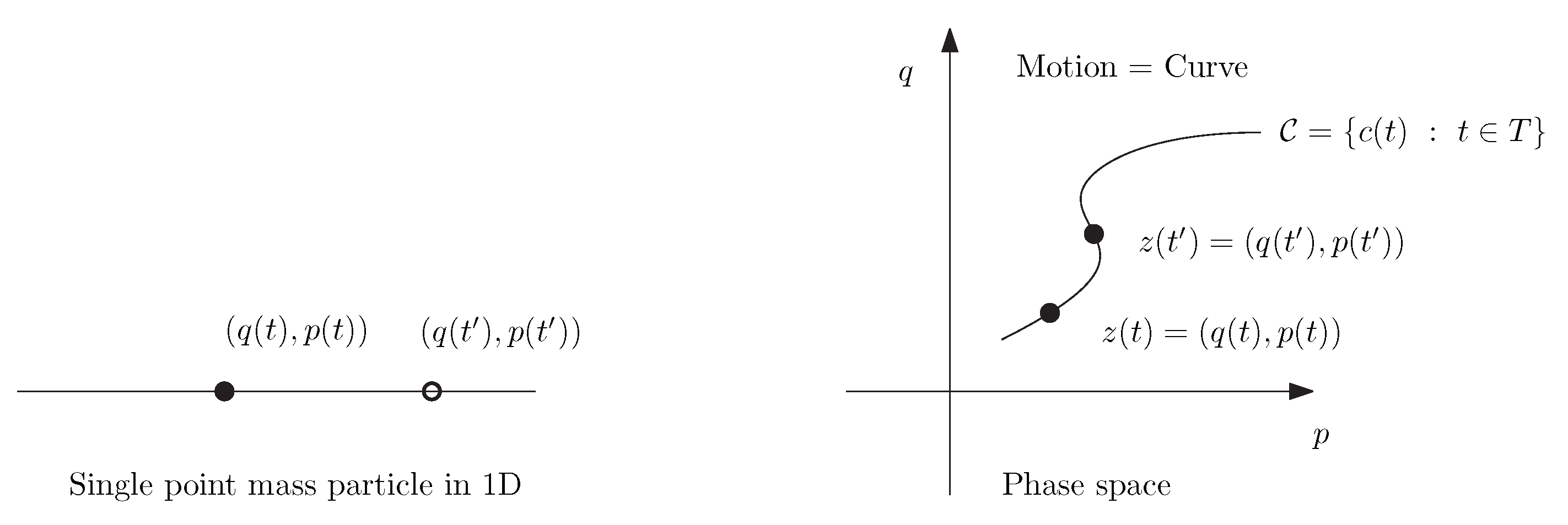
Figure 2.
Interpreting a 2D symplectic form as the signed area of a parallelogram with first oriented edge (grey). A pair of vectors defines two possible orientations of the parallelogram: The orientation compatible with and the reverse orientation compatible with . is called the standard area form.

Figure 3.
Bregman divergences generalized to dual systems : A symplectic form on the space is induced by the pairing product. The Bregman divergence on the dual system is then defined as the symplectic Bregman divergence on the symplectic vector space .
Figure 3.
Bregman divergences generalized to dual systems : A symplectic form on the space is induced by the pairing product. The Bregman divergence on the dual system is then defined as the symplectic Bregman divergence on the symplectic vector space .

Disclaimer/Publisher’s Note: The statements, opinions and data contained in all publications are solely those of the individual author(s) and contributor(s) and not of MDPI and/or the editor(s). MDPI and/or the editor(s) disclaim responsibility for any injury to people or property resulting from any ideas, methods, instructions or products referred to in the content. |
© 2024 by the author. Licensee MDPI, Basel, Switzerland. This article is an open access article distributed under the terms and conditions of the Creative Commons Attribution (CC BY) license (https://creativecommons.org/licenses/by/4.0/).
Share and Cite
MDPI and ACS Style
Nielsen, F. Symplectic Bregman Divergences. Entropy 2024, 26, 1101. https://doi.org/10.3390/e26121101
AMA Style
Nielsen F. Symplectic Bregman Divergences. Entropy. 2024; 26(12):1101. https://doi.org/10.3390/e26121101
Chicago/Turabian StyleNielsen, Frank. 2024. "Symplectic Bregman Divergences" Entropy 26, no. 12: 1101. https://doi.org/10.3390/e26121101
APA StyleNielsen, F. (2024). Symplectic Bregman Divergences. Entropy, 26(12), 1101. https://doi.org/10.3390/e26121101
Note that from the first issue of 2016, this journal uses article numbers instead of page numbers. See further details here.