
LPI Radar Waveform Recognition Based on Hierarchical Classification Approach and Maximum Likelihood Estimation

Abstract
1. Introduction
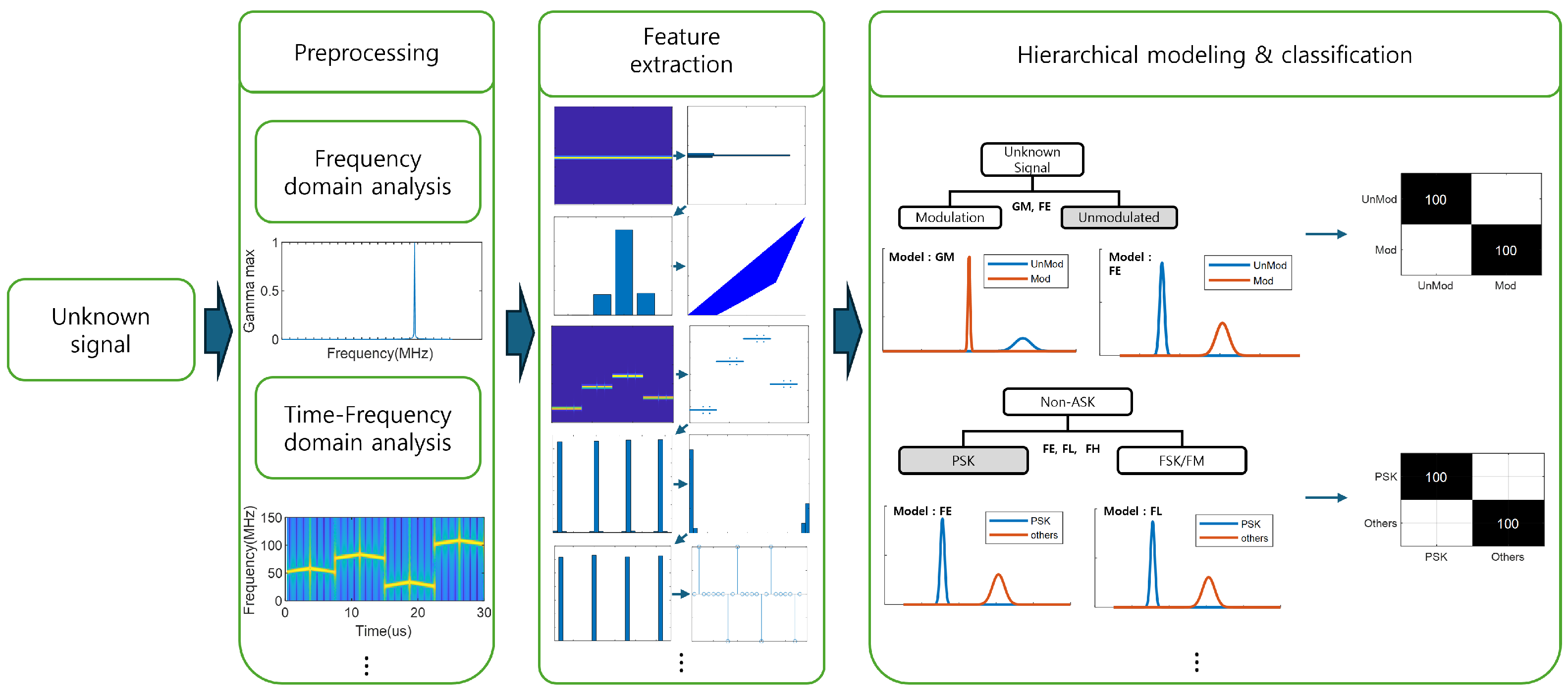
2. Proposed Methods
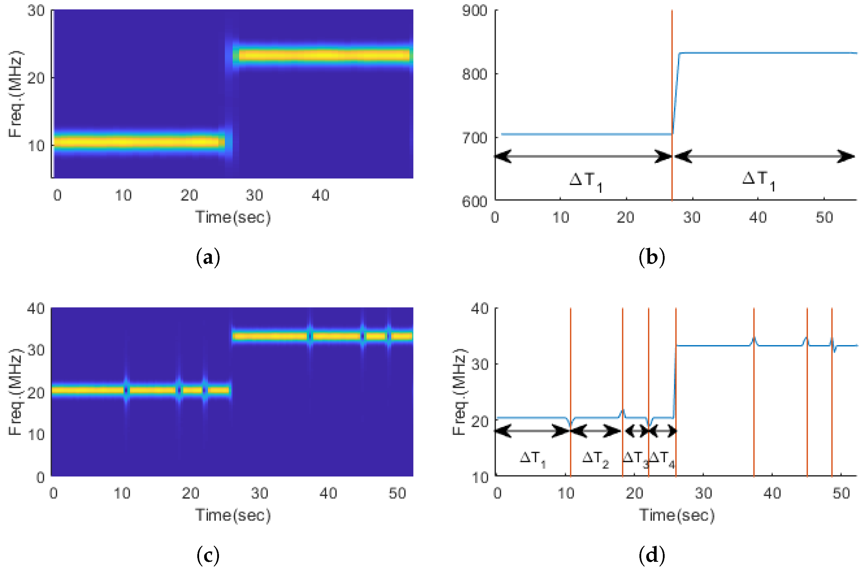
2.1. Time–Frequency Transformation
2.2. Feature Extraction
2.2.1. Gamma Max (GM)
2.2.2. Gini’s Coefficient (GC)
2.2.3. Frequency Entropy (FE)
2.2.4. Frequency Level (FL)
2.2.5. Frequency Hopping (FH)
2.2.6. Inter-Pulse Entropy (ITE)/Inter-Pulse Gini’s Coefficient (ITG)
2.2.7. Intra-Pulse Entropy (INE)/Intra-Pulse Gini’s Coefficient (ING)
2.2.8. Nullity
2.2.9. Non-Linearity
2.3. Classifier Design
- Level 0: Distinction between modulated and UnMod signals;
- Level 1: Distinction between PSK, FSK, FM, and ASK;
- Level 2-1: Distinction between PSK and FSK, FM;
- Level 2-2: Distinction between LFM-ASK and NLFM-ASKl
- Level 3: Distinction between FSK and FM;
- Level 4-1: Distinction between FSK, FSK-FM and FSK-PSK;
- Level 4-2: Distinction between FM-PSK and FM;
- Level 5-1: Distinction between FSK and FSK-FM;
- Level 5-2: Distinction between 2FSK-PSK, 3FSK-PSK, 8FSK-PSK and FSKC-PSK;
- Level 5-3: Distinction between LFM-PSK, NLFM2-PSK, NLFM3-PSK and NLFMS-PSK;
- Level 5-4: Distinction between LFM, NLFM2, NLFM3 and NLFMS;
- Level 6-1: Distinction between M-ary FSK and FSKC;
- Level 6-2: Distinction between FSK-LFM and FSK-NLFM;
- Level 7: Distinction between 2FSK, 3FSK and 8FSK.
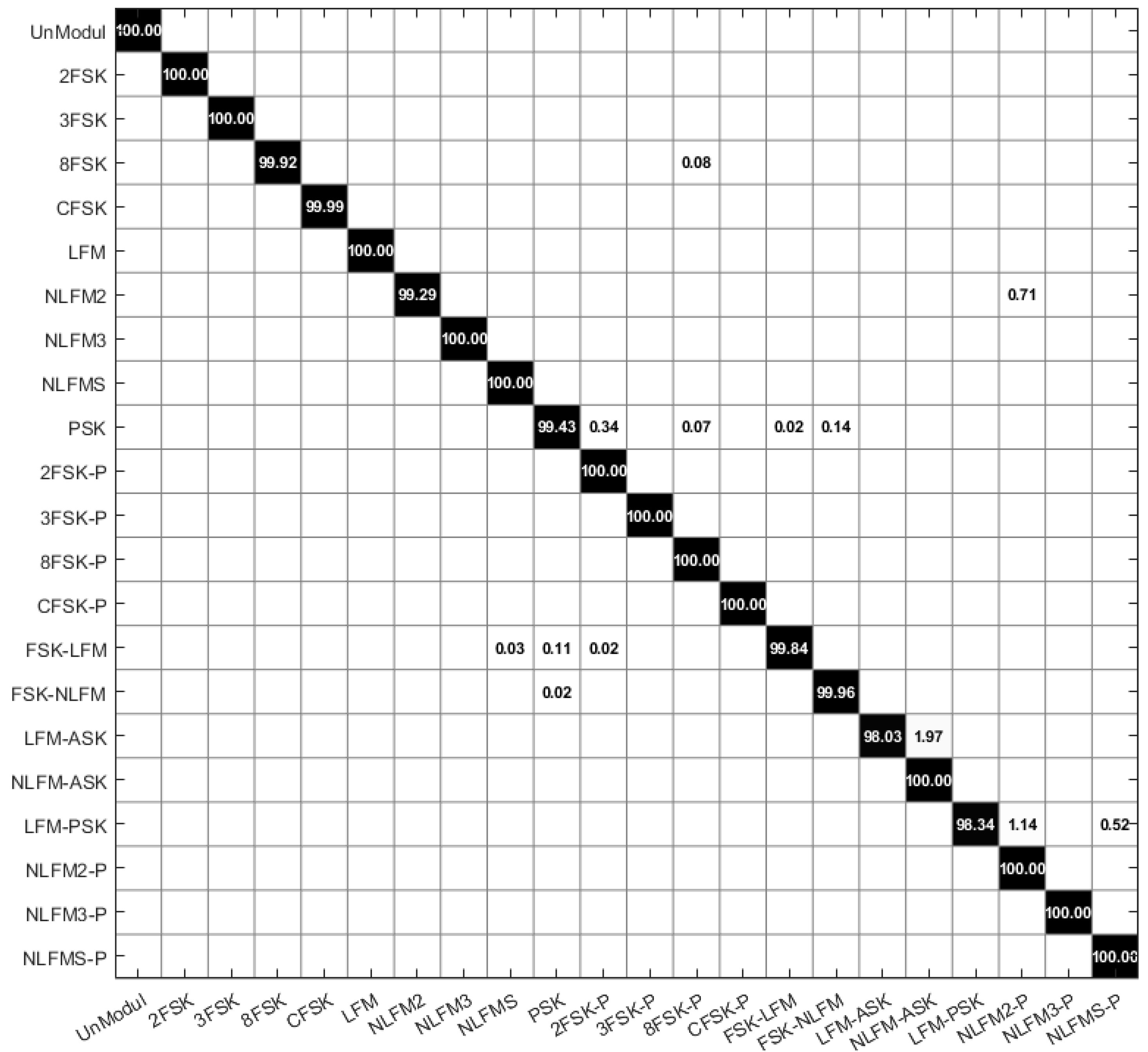
3. Experimental Result
4. Conclusions
Author Contributions
Funding
Institutional Review Board Statement
Informed Consent Statement
Data Availability Statement
Conflicts of Interest
Abbreviations
| ASK | Amplitude Shift Keying |
| AWGN | Additive White Gaussian Noise |
| CNN | Convolution Neural Network |
| CWD | Choi–Williams Distribution |
| DCNN | Deep Convolutional Neural Network |
| DQN | Deep Q-Network |
| FE | Frequency Entropy |
| FF-CNN | deep Fused Fully Convolutional Neural Network |
| FH | Frequency Hopping |
| FL | Frequency Level |
| FM | Frequency Modulation |
| FSK | Frequency Shift Keying |
| GC | Gini’s Coefficient |
| GM | Gamma Max |
| INE | Intra-Pulse Entropy |
| ING | Intra-Pulse Gini’s coefficient |
| ITE | Inter-Pulse Entropy |
| ITG | Inter-Pulse Gini’s coefficient |
| kNN | k-Nearest Neighbor |
| LFM | Linear FM |
| MLE | Maximum Likelihood Estimation |
| NLFM | Non-Linear FM |
| PSK | Phase Shift Keying |
| STFT | Short-Time Fourier Transform |
| SVM | Support Vector Machine |
| UnMod | UnModulated signal |
| WVD | Wigner–Ville Distribution |
References
- Adamy, D.L. EW 101, a First Course in Electronic Warfare; Artech House: Washington, DC, USA, 2008. [Google Scholar]
- Adamy, D. EW 102: A Second Course in Electronic Warfare; Artech House: Washington, DC, USA, 2004. [Google Scholar]
- Blunt, S.D.; Yatham, P.; Stiles, J. Intrapulse radar-embedded communications. IEEE Trans. Aerosp. Electron. Syst. 2010, 46, 1185–1200. [Google Scholar] [CrossRef]
- Ciuonzo, D.; De Maio, A.; Foglia, G.; Piezzo, M. Intrapulse radar-embedded communications via multiobjective optimization. IEEE Trans. Aerosp. Electron. Syst. 2015, 51, 2960–2974. [Google Scholar] [CrossRef]
- Pace, P.E. Detecting and Classifying Low Probability of Intercept Radar; Artech House: Washington, DC, USA, 2009. [Google Scholar]
- Bishop, C.M.; Nasrabadi, N.M. Pattern Recognition and Machine Learning; Springer: Berlin/Heidelberg, Germany, 2006; Volume 4. [Google Scholar]
- Wan, T.; Jiang, K.; Tang, Y.; Xiong, Y.; Tang, B. Automatic LPI radar signal sensing method using visibility graphs. IEEE Access 2020, 8, 159650–159660. [Google Scholar] [CrossRef]
- Kishore, T.R.; Rao, K.D. Automatic intrapulse modulation classification of advanced LPI radar waveforms. IEEE Trans. Aerosp. Electron. Syst. 2017, 53, 901–914. [Google Scholar] [CrossRef]
- Ma, X.; Liu, D.; Shan, Y. Intra-pulse modulation recognition using short-time ramanujan Fourier transform spectrogram. EURASIP J. Adv. Signal Process. 2017, 2017, 42. [Google Scholar] [CrossRef]
- Chen, K.; Chen, S.; Zhang, S.; Zhao, H. Automatic modulation recognition of radar signals based on histogram of oriented gradient via improved principal component analysis. Signal Image Video Process. 2023, 17, 3053–3061. [Google Scholar] [CrossRef]
- Kelleher, J.D. Deep Learning; MIT Press: Cambridge, MA, USA, 2019. [Google Scholar]
- Chen, K.; Zhang, S.; Zhu, L.; Chen, S.; Zhao, H. Modulation recognition of radar signals based on adaptive singular value reconstruction and deep residual learning. Sensors 2021, 21, 449. [Google Scholar] [CrossRef] [PubMed]
- Si, W.; Wan, C.; Deng, Z. Intra-pulse modulation recognition of dual-component radar signals based on deep convolutional neural network. IEEE Commun. Lett. 2021, 25, 3305–3309. [Google Scholar] [CrossRef]
- Qu, Z.; Hou, C.; Hou, C.; Wang, W. Radar signal intra-pulse modulation recognition based on convolutional neural network and deep Q-learning network. IEEE Access 2020, 8, 49125–49136. [Google Scholar] [CrossRef]
- Akyon, F.C.; Alp, Y.K.; Gok, G.; Arikan, O. Classification of intra-pulse modulation of radar signals by feature fusion based convolutional neural networks. In Proceedings of the 2018 26th European Signal Processing Conference (EUSIPCO), Rome, Italy, 3–7 September 2018; pp. 2290–2294. [Google Scholar]
- Bhatti, S.G.; Bhatti, A.I. Radar signals intrapulse modulation recognition using phase-based stft and bilstm. IEEE Access 2022, 10, 80184–80194. [Google Scholar] [CrossRef]
- Chen, K.; Zhang, J.; Chen, S.; Zhang, S.; Zhao, H. Automatic modulation classification of radar signals utilizing X-net. Digit. Signal Process. 2022, 123, 103396. [Google Scholar] [CrossRef]
- Pan, J.X.; Fang, K.T.; Pan, J.X.; Fang, K.T. Maximum likelihood estimation. In Growth Curve Models and Statistical Diagnostics; Springer Science & Business Media: Berlin, Germany, 2002; pp. 77–158. [Google Scholar]
- Xiang, L.; Hu, A. Comparison of Methods for Different Time-frequency Analysis of Vibration Signal. J. Softw. 2012, 7, 68–74. [Google Scholar] [CrossRef]
- Singh, V.K.; Pachori, R.B. Sliding eigenvalue decomposition-based cross-term suppression in Wigner–Ville distribution. J. Comput. Electron. 2021, 20, 2245–2254. [Google Scholar] [CrossRef]
- Azzouz, E.; Nandi, A. Automatic Modulation Recognition of Communication Signals; Springer: Berlin/Heidelberg, Germany, 1996. [Google Scholar]
- Dorfman, R. A formula for the Gini coefficient. Rev. Econ. Stat. 1979, 61, 146–149. [Google Scholar] [CrossRef]
- Gray, R.M. Entropy and Information Theory; Springer Science & Business Media: Cham, Switzerland, 2011. [Google Scholar]


| Description | |
|---|---|
| GM | Maximum power of the spectrum. Useful for distinguishing between Mod and UnMod |
| GC | Indicates how evenly the frequencies are distributed. Useful for distinguishing between FSK and FM, as well as between LFM, NLFM2, NLFM3, and NLFMS. |
| FL | Indicates the number of frequency shifts. Used to distinguish M-ary FSK signals |
| FE | Quantifies the uncertainty of the frequency. Used to distinguish between PSK and FSK, FM signals, as well as between FSK and FM signals. |
| FH | Quantifies the random change in frequency using Gini’s coefficient. Used to distinguish between PSK and FSK, FM signals |
| NL | Quantifies whether the instantaneous frequency increases or decreases linearly over time. Used to distinguish between LFM and NLFM signals |
| ITE | Quantifies, using information entropy, how evenly the lengths of the intervals where the phase does not change within a pulse are distributed. Useful for distinguishing whether there is hybrid modulation with a PSK signal or not. |
| ITG | Quantifies, using Gini’s coefficient (GC), how evenly the lengths of the intervals where the phase does not change within a pulse are distributed. Useful for distinguishing whether there is hybrid modulation with a PSK signal or not. |
| INE | Quantifies, using information entropy, whether the frequency increases or decreases within a symbol. Useful for distinguishing whether there is hybrid modulation with an FM signal or not. |
| ING | Quantifies, using Gini’s coefficient (GC), whether the frequency increases or decreases within a symbol. Useful for distinguishing whether there is hybrid modulation with an FM signal or not. |
| Nullity | Proportion of intervals where no frequency is present within the signal. Useful for distinguishing whether there is hybrid modulation with an ASK signal or not. |
| Modulation | Parameter | Value |
|---|---|---|
| Unmodulated | 20 | |
| 10,50,100 | ||
| 2FSK 3FSK | 20 | |
| 5, 10 | ||
| 2, 5 | ||
| 50, 100, 200 | ||
| 8FSK FSK Costas | 20 | |
| 1, 2, 5 | ||
| 2, 5 | ||
| 50, 100, 200 | ||
| LFM | 20 | |
| 20, 30, 40 | ||
| 50, 100, 200 | ||
| 0, 0.5, 1.0 | ||
| NLFM2 NLFM3 NLFMS | 20 | |
| 20, 30, 40 | ||
| 50, 100, 200 | ||
| PSK-Barker code | 20 | |
| N | 7,11,13 | |
| 0.5, 1, 2, 5 | ||
| PSK-PN code | 20 | |
| N | 31, 63, 127 | |
| 0.5, 1, 2, 5 | ||
| PSK-Taylor code | 10 | |
| N | 13, 28 | |
| 0.5, 1, 2, 5 | ||
| PSK-Frank code PSK P1, P2 code | 20 | |
| M | 4, 8, 16 | |
| 0.5, 1, 2, 5 | ||
| PSK P3, P4 code | 20 | |
| N | 16, 64, 256 | |
| 0.5, 1, 2, 5 | ||
| PSK T1, T2 code | 20 | |
| n | 2, 4, 8 | |
| s | 4, 8, 16 | |
| 0.5, 1, 2, 5 | ||
| 64, 128, 256 |
| Internal External | Parameter | Value |
|---|---|---|
| PSK-Barker 2FSK or 3FSK | N | 7, 11, 13 |
| 20 | ||
| 5, 10 | ||
| PSK-Barker 8FSK | N | 7, 11, 13 |
| 20 | ||
| 25 | ||
| PSK-Barker FSK Costas | N | 7, 11, 13 |
| 20 | ||
| 5 | ||
| LFN, NLFM 2FSK or 3FSK | /2, /4 | |
| 0, 0.5, 1 | ||
| 20 | ||
| 5,10 | ||
| 5, 10 | ||
| 50, 100, 200 | ||
| LFN, NLFM 8FSK | /2, /4 | |
| 0, 0.5, 1 | ||
| 20 | ||
| 25 | ||
| 5, 10 | ||
| 50, 100, 200 | ||
| LFN, NLFM Costas FSK | /2, /4 | |
| 0, 0.5, 1 | ||
| 20 | ||
| 5 | ||
| 5, 10 | ||
| 50, 100, 200 | ||
| ASK LFN, NLFM | symbol length | 2, 5 |
| 20 | ||
| 20, 30, 40 | ||
| 50, 100, 200 | ||
| 0, 0.5, 1 | ||
| PSK-Barker LFN, NLFM | code length | 7, 11, 13 |
| 2, 5 | ||
| 20 | ||
| 20, 30, 40 | ||
| 50, 100, 200 | ||
| 0, 0.5, 1 |
| Authors | Kinds of LPI Radar Waveforms | Method | Noise Level | Average Accuracy |
|---|---|---|---|---|
| Wan, T. et al. [7] | 18 | kNN + SVM | 0 dB | 97.40% |
| Kishore, T.R. et al. [8] | 9 | Binary tree | −10 dB | 90% |
| Ma, X. et al. [9] | 5 | Binary tree + kNN | −5 dB | 90% |
| Chen, K. et al. [10] | 8 | IPCA + SVM | −6 dB | 97.37% |
| Chen, K. et al. [12] | 8 | Deep residual learning | −8 dB | 94.1% |
| Si, W. et al. [13] | 4 | DCNN | −8 dB | 96.17% |
| Qu, Z. et al [14] | 8 | CNN + DQN | −6 dB | 94.83% |
| Akyon, F.C. et al. [15] | 23 | FF-CNN | 5 dB | 99.85% |
| Bhatti, S.G. et al. [16] | 6 | BiLSTM | −2 dB | 90% |
| Chen, K. et al. [17] | 10 | BLCDAE + X-net | −8 dB | 96% |
| Proposed | 47 | Hierarchical classification + MLE | 8 dB | 98.45% |
Disclaimer/Publisher’s Note: The statements, opinions and data contained in all publications are solely those of the individual author(s) and contributor(s) and not of MDPI and/or the editor(s). MDPI and/or the editor(s) disclaim responsibility for any injury to people or property resulting from any ideas, methods, instructions or products referred to in the content. |
© 2024 by the authors. Licensee MDPI, Basel, Switzerland. This article is an open access article distributed under the terms and conditions of the Creative Commons Attribution (CC BY) license (https://creativecommons.org/licenses/by/4.0/).
Share and Cite
Rhee, K.; Baik, J.; Song, C.; Shin, H.-C. LPI Radar Waveform Recognition Based on Hierarchical Classification Approach and Maximum Likelihood Estimation. Entropy 2024, 26, 915. https://doi.org/10.3390/e26110915
Rhee K, Baik J, Song C, Shin H-C. LPI Radar Waveform Recognition Based on Hierarchical Classification Approach and Maximum Likelihood Estimation. Entropy. 2024; 26(11):915. https://doi.org/10.3390/e26110915
Chicago/Turabian StyleRhee, Kiwon, Jaeyoung Baik, Changhoon Song, and Hyun-Chool Shin. 2024. "LPI Radar Waveform Recognition Based on Hierarchical Classification Approach and Maximum Likelihood Estimation" Entropy 26, no. 11: 915. https://doi.org/10.3390/e26110915
APA StyleRhee, K., Baik, J., Song, C., & Shin, H.-C. (2024). LPI Radar Waveform Recognition Based on Hierarchical Classification Approach and Maximum Likelihood Estimation. Entropy, 26(11), 915. https://doi.org/10.3390/e26110915