
Efficient Multi-Change Point Analysis to Decode Economic Crisis Information from the S&P500 Mean Market Correlation


Abstract
1. Introduction
2. Data and Methods
2.1. Data Preparation
2.2. Change Point Identification
3. Results
3.1. Change Point Analysis
3.1.1. Dot-Com Bubble
3.1.2. Financial Crisis
3.1.3. Euro Crisis

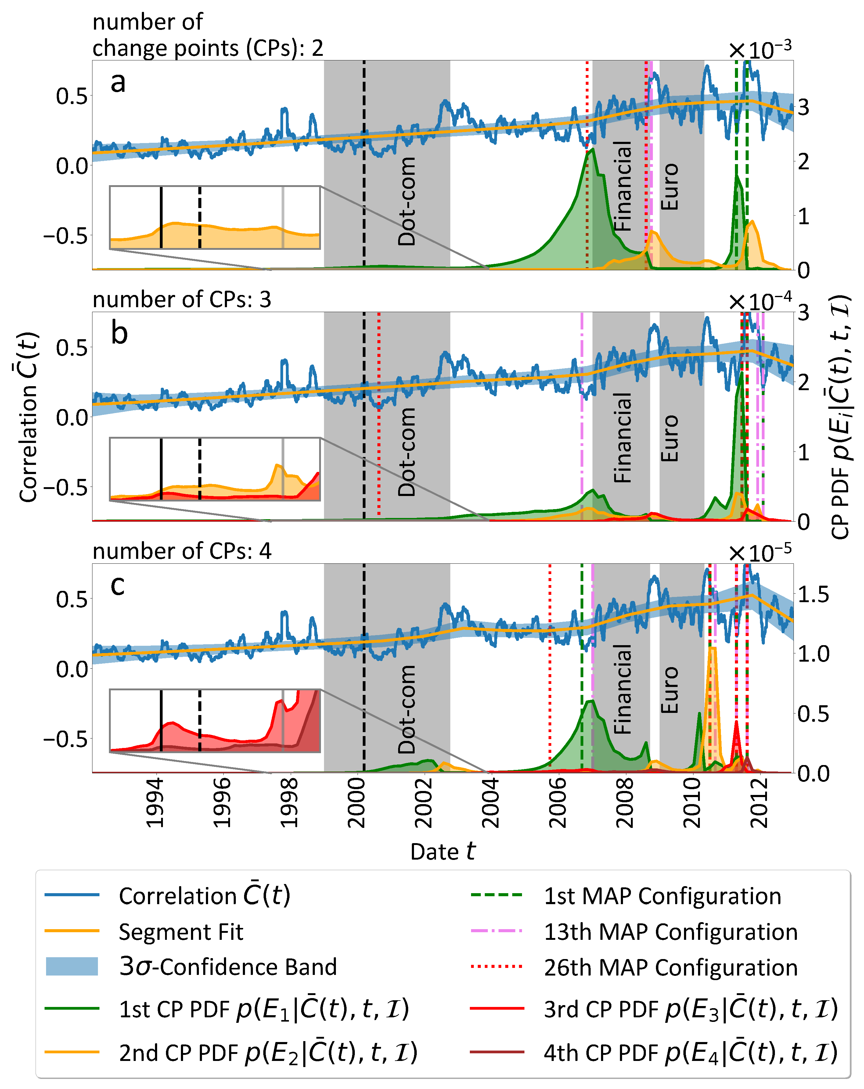
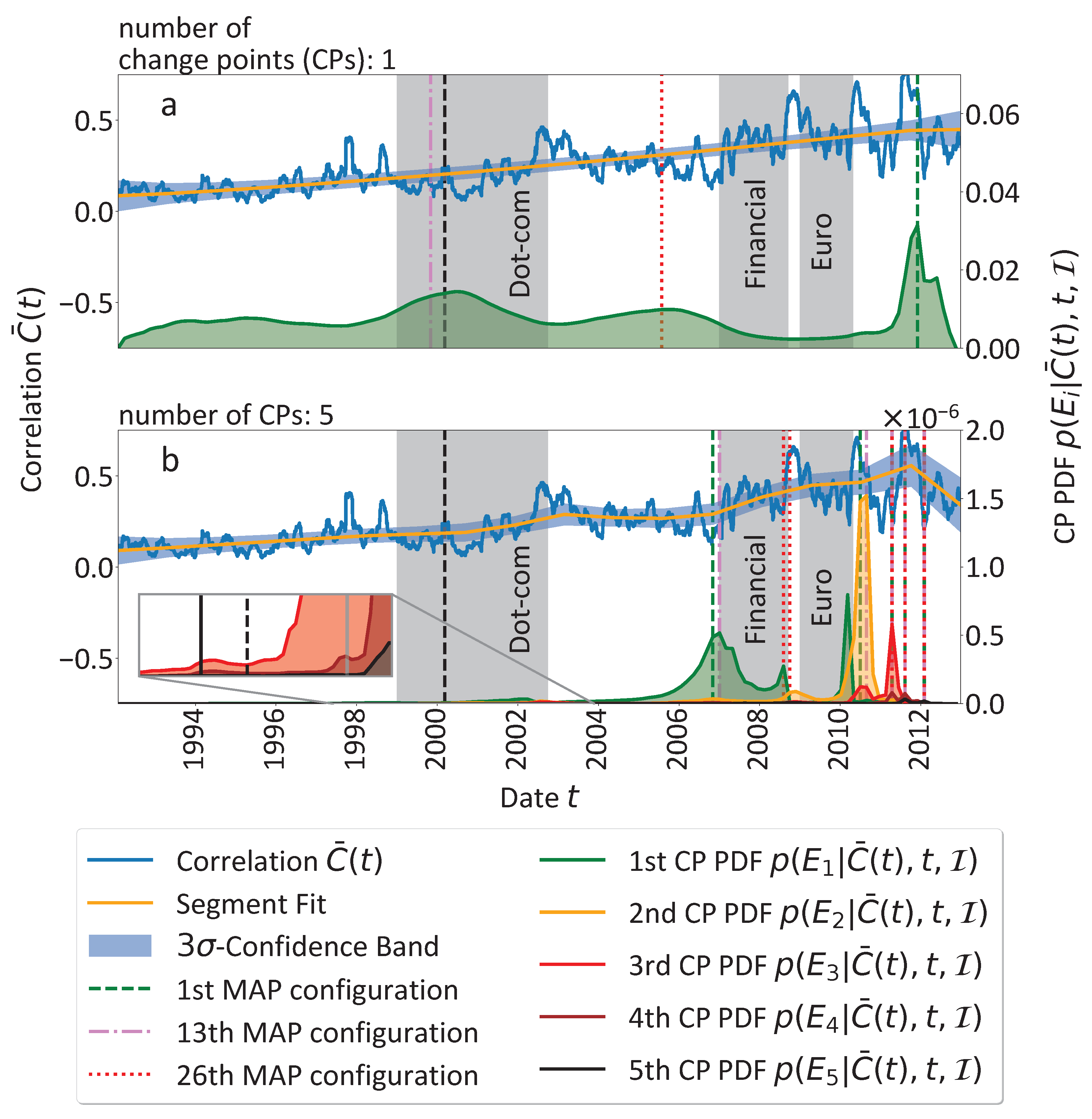
| Event Date | Event Description | Source | CP PDF Peak Dates | ||
|---|---|---|---|---|---|
| Figure 2a | Figure 2b | Figure 2c | |||
| 1994 | Over the year, bond prices fell continuously in consequence of partially unexpected and repeated raise of federal funds rates by the FED. In consequence bonds lost about USD 1.5 trillion in market value globally. | [28] | 2 February 1995 to 26 July 1995; 31 March 1995 to 21 September 1995 | 2 February 1995; 31 March 1995 to 21 September 1995 | 26 July 1995 to 16 November 1995; 2 February 1995; 26 July 1995 to 16 November 1995 |
| December 1994 | Due to devaluation of the peso by the Mexican government and thus anticipating further devaluations, investors rapidly withdrew capital from Mexican investments. In January 1995 the U.S. government coordinates a USD 40 billion bailout. | [29] | 2 February 1995 to 26 July 1995; 31 March 1995 to 21 September 1995 | 2 February 1995; 31 March 1995 to 21 September 1995 | 26 July 1995 to 16 November 1995; 2 February 1995; 26 July 1995 to 16 November 1995 |
| 1997–1998 | Asian financial crisis in East and Southeast Asia. Multiple origins are discussed. However, long-lasting global contagion stayed away and the markets recovered fast in 1998–1999. | [20] | 14 May 1999 | 10 October 1997; 18 March 1999 | 10 October 1997; 18 March 1999; 14 May 1999 |
| 1998–1999 | Russian financial crisis in which the ruble was devalued. As a result, many neighbouring countries experienced also severe crises. | [21] | 14 May 1999 | 18 March 1999 to 13 July 1999 | 18 March 1999; 14 May 1999 |
| 1 January 1999 | The modest onset of the dot-com bubble 1998 turns into a rapid rally of the NASDAQ Composite Index. In the literature the long pre-bubble period begins commonly in 1995. | [30,31] | 14 May 1999 | 18 March 1999 to 12 July 1999 | 18 March 1999 |
| 14 May 1999 | Stock market drop due to sharp rise of consumer prices to 1.75% in the U.S. | [19] | 14 May 1999 | 14 May 1999 to 12 July 1999 | 14 May 1999 |
| 10 March 2000 | Based on the NASDAQ Composite Index the Dot-com bubble reaches its all-time high. | [30,31] | 16 October 2000 | 22 June 2000; 9 April 2001 | kink at 22 June 2000; 9 April 2001 |
| 11 September 2001 | In course of a terror attack three airplanes crash into the twin towers of the U.S. World Trade Center and the Pentagon coordinated by the militant Islamist extremist network al-Qaeda. | [18] | 24 May to 23 July 2002 | 4 October 2001; 24 May 2002; 23 July 2002 | 4 October 2001; 30 January 2002; 24 May 2002; 23 July 2002; 18 September 2002 |
| 1 October 2002 | Based on the NASDAQ Composite Index the Dot-com bubble reaches a new trough after the bubble burst in course of a more general stock downturn since 11 September 2011. | [30,31] | 28 July 2005 to 18 November 2005 | 28 October 2003 to 24 December 2003 | 28 October 2003 to 24 December 2003 |
| 2002/2003 | The Venezuelan General Strike massively hinders oil exports among others to the USA. | [32,33] | 28 July 2005 to 18 November 2005 | 28 October 2003 to 24 December 2003 | 28 October 2003 to 24 December 2003 |
| 2003 | Approximate beginning of the boom-phase of the U.S. housing bubble. | [34] | 28 July 2005 to 18 November 2005 | 28 October 2003 to 24 December 2003 | 28 October 2003 to 24 December 2003 |
| 2003–2016 | Begin of rising oil prices from under USD 25/bbl to above USD 30/bbl. The peak of USD 147.30/bbl is reached in July 2008, before they return temporarily to USD 35/bbl in 2009. | [33,35] | 28 July 2005 to 18 November 2005 | 28 October 2003 to 24 December 2003 | 28 October 2003 to 24 December 2003 |
| Q4 2006 to Q1 2007 | Period of most intense burst of the U.S. housing bubble with new lowest price in 2011. | [22] | 2 November 2006 to 3 January 2007 | 31 October 2006; 2 January 2007 | 2 November 2006 to 3 January 2007 |
| 9 August 2007 | Commonly listed onset of the global financial crisis. On this day the interest rates for inter-bank financial loans rose sharply. | [23,24] | 22 August 2007 | 22 August 2007 | 22 August 2007 |
| 2008 | Year of the financial crisis and great recession. The year is characterised by manifold bailouts for banks and stock market crashes. | [36] | overall high CP PDFs in 2008 | overall high CP PDFs in 2008 | overall high CP PDFs in 2008 |
| January to March 2008 | The housing prices continue to collapse. The government passes a tax rebate bill on 13 February 2008 and the FED starts bailout programs in the beginning of March. | [37,38] | 4 August 2008 | 4 August 2008 | 4 August 2008 |
| 30 July 2008 | U.S. governments passes bailout laws for Fanny Mae and Freddie Mac. | [39] | Kink at 4 August 2008 | 4 August 2008 | 4 August 2008 |
| 7 September 2008 | U.S. government’s take over of Fanny Mae Association and Freddie Mac Corporation. | [40] | 1 October 2008 to 26 November 2008 | 1 October 2008 | 1 October 2008 to 26 November 2008 |
| 15 September 2008 | Lehman Brothers bankruptcy. | [25] | 1 October 2008 | 1 October 2008 | 1 October 2008 |
| 29 September 2008 | Stock market collapsed when the bailout bill was rejected by the U.S. House of Representatives. | [26] | 1 October 2008 | 30 September 2008 | 1 October 2008 |
| 24 October 2008 | Many world stock indices lost around 10%. | [41] | 26 November 2008 | 26 November 2008 | 26 November 2008 |
| 1 December 2008 | When the National Bureau of Economic Research officially declared that the U.S. was in a recession since December 2007, the S&P500 lost 8.93% and the financial stocks of the index even 17% based on these news. | [42] | high CP PDF after 26 November 2008 | high CP PDF after 26 November 2008 | high CP PDF after 26 November 2008 |
| January 2009 | The first ten European banks ask for bailout programs. | [43] | high CP PDF after 26 November 2008 | high CP PDF after 26 November 2008 | high CP PDF after 26 November 2008 |
| Early 2010 to mid 2012 | The Arab Spring. Great anti-government protests in large parts of the Middle East and North Africa. The oil prices rise above USD 100/bbl. | [35,44,45] | 5 May 2010 to 1 July 2010 | 5 May 2010 to 1 July 2010 | 5 May 2010 to 1 July 2010 |
| 27 April 2010 | Greece’s sovereign debt rating was downgraded by Standard& Poor’s. | [27] | 5 May 2010 to 1 July 2010 | 5 May 2010 to 1 July 2010 | 5 May 2010 to 1 July 2010 |
| 6 May 2010 | So-called flash crash led to a 9% drop in the Dow Jones Index caused due to high frequency trading. | [46] | 5 May 2010 to 1 July 2010 | 5 May 2010 to 1 July 2010 | 5 May 2010 to 1 July 2010 |
| 8 May 2010 | Passing drastic bailout plans for Greece in Brussels. A EUR 110 billion package is approved. | [47,48] | 5 May 2010 to 1 July 2010 | 5 May 2010 to 1 July 2010; 28 August 2010 | 5 May 2010 to 1 July 2010; 1 July to 28 August 2010 |
| 17 May 2010 | The Euro currency falls into first four-years low. | [49] | 5 May 2010 to 1 July 2010 | 5 May 2010 to 1 July 2010; 28 August 2010 | 5 May 2010 to 1 July 2010; 1 July to 28 August 2010 |
| Q1/2 2010 | Several downgradings of debt ratings/bonds of European countries, i.e., Portugal, Spain, Greece. | [50] | 5 May 2010 to 1 July 2010 | 5 May 2010 to 1 July 2010; 28 August 2010 | 5 May 2010 to 1 July 2010; 1 July to 28 August 2010 3 September 2010 |
| 4 June 2010 | The Euro currency falls into a second four-year low. Major American markets fall more than 3%. | [51] | 5 May 2010 to 1 July 2010 | 5 May 2010 to 1 July 2010; 28 August 2010 | 5 May 2010 to 1 July 2010; 1 July to 28 August 2010 |
| November 2010 | Bailout request by Ireland. At the end of November Ireland receives EUR 85 billion. | [52,53] | 15 April 2011 | 15 April 2011 | 15 April 2011 |
| 7 April 2011 | In the evening of 6 April 2011 Portugal’s government announces that it is the third after Greece’s and Ireland’s governments that will ask for a bailout package. On 17 May 2011 a bailout package of around EUR 78 billion is formally adopted. | [54] | 15 April 2011 to 14 June 2011 | 15 April 2011 to 14 June 2011 | 15 May 2011 to 14 June 2011 |
| 13 June 2011 | Greece’s credit rankings become worst in the world. | [55] | 13 June 2011 | 13 June 2011 | 13 June 2011 |
| August 2011 | Under the Securities Markets Programme the ECB restarts to purchase a significant amount of eurozone sovereign bonds. Spanish and Italian yields breach 6%. | [56,57] | 6 October 2011 | 9/10 August 2011 | 10 August 2011 |
3.1.4. Remarks and Intermediate Conclusion
3.2. On-Line Change Point Evolution in Pre-Crisis-Segments
3.2.1. Dot-Com Bubble
3.2.2. Financial Crisis
3.2.3. Euro Crisis
4. Discussion and Conclusions
Author Contributions
Funding
Institutional Review Board Statement
Data Availability Statement
Acknowledgments
Conflicts of Interest
Abbreviations
| CB | Confidence Band |
| CP | Change Point |
| ECB | European Central Bank |
| FED | U.S. Federal Reserve System |
| NASDAQ | National Association of Securities Dealers Automated Quotations |
| U.S. | United States |
| USA | United States of America |
| probability density function | |
| Q1, Q2, … | quarter 1, quarter 2, … |
| S&P | Standard and Poor’s |
Appendix A. Detailed Data Preparation

Appendix B. Advanced Change Point Analysis
References
- Stepanov, Y.; Rinn, P.; Guhr, T.; Peinke, J.; Schäfer, R. Stability and hierarchy of quasi-stationary states: Financial markets as an example. J. Stat. Mech. Theory Exp. 2015, 2015, P08011. [Google Scholar] [CrossRef]
- Laloux, L.; Cizeau, P.; Bouchaud, J.P.; Potters, M. Noise Dressing of Financial Correlation Matrices. Phys. Rev. Lett. 1999, 83, 1467–1470. [Google Scholar] [CrossRef]
- Plerou, V.; Gopikrishnan, P.; Rosenow, B.; Nunes Amaral, L.A.; Stanley, H.E. Universal and Nonuniversal Properties of Cross Correlations in Financial Time Series. Phys. Rev. Lett. 1999, 83, 1471–1474. [Google Scholar] [CrossRef]
- Kwapień, J.; Drożdż, S. Physical approach to complex systems. Phys. Rep. 2012, 515, 115–226. [Google Scholar] [CrossRef]
- Pharasi, H.K.; Sharma, K.; Chakraborti, A.; Seligman, T.H. Complex market dynamics in the light of random matrix theory. arXiv 2018, arXiv:1809.07100. [Google Scholar]
- Münnix, M.C.; Shimada, T.; Schäfer, R.; Leyvraz, F.; Seligman, T.H.; Guhr, T.; Stanley, H.E. Identifying States of a Financial Market. Sci. Rep. 2012, 2, 644. [Google Scholar] [CrossRef]
- Rinn, P.; Stepanov, Y.; Peinke, J.; Guhr, T.; Schäfer, R. Dynamics of quasi-stationary systems: Finance as an example. EPL (Europhys. Lett.) 2015, 110, 68003. [Google Scholar] [CrossRef]
- Heckens, A.J.; Guhr, T. A new attempt to identify long-term precursors for endogenous financial crises in the market correlation structures. J. Stat. Mech. Theory Exp. 2022, 2022, 043401. [Google Scholar] [CrossRef]
- Heckens, A.J.; Krause, S.M.; Guhr, T. Uncovering the dynamics of correlation structures relative to the collective market motion. J. Stat. Mech. Theory Exp. 2020, 2020, 103402. [Google Scholar] [CrossRef]
- Heckens, A.J.; Guhr, T. New collectivity measures for financial covariances and correlations. Phys. A Stat. Mech. Its Appl. 2022, 604, 127704. [Google Scholar] [CrossRef]
- Dehning, J.; Zierenberg, J.; Spitzner, F.P.; Wibral, M.; Neto, J.P.; Wilczek, M.; Priesemann, V. Inferring change points in the spread of COVID-19 reveals the effectiveness of interventions. Science 2020, 369, eabb9789. [Google Scholar] [CrossRef] [PubMed]
- Wand, T.; Heßler, M.; Kamps, O. Memory Effects, Multiple Time Scales and Local Stability in Langevin Models of the S&P500 Market Correlation. Entropy 2023, 25, 1257. [Google Scholar] [CrossRef]
- Heßler, M.; Kamps, O. Bayesian online anticipation of critical transitions. New J. Phys. 2021, 24, 063021. [Google Scholar] [CrossRef]
- Heßler, M. antiCPy. Zenodo 2021. [Google Scholar] [CrossRef]
- Heßler, M. antiCPy’s Documentation. 2021. Available online: https://anticpy.readthedocs.io (accessed on 23 August 2023).
- Dose, V.; Menzel, A. Bayesian analysis of climate change impacts in phenology. Glob. Chang. Biol. 2004, 10, 259–272. [Google Scholar] [CrossRef]
- Von der Linden, W.; Dose, V.; Von Toussaint, U. Bayesian Probability Theory: Applications in the Physical Sciences; Cambridge University Press: Cambridge, UK, 2014. [Google Scholar]
- Kean, T.H.; Ben-Veniste, R.; Fielding, F.F.; Gorelick, J.S.; Gorton, S.; Hamilton, L.H.; Kerrey, B.; Lehman, J.F.; Roemer, T.J.; Thompson, J.R. The 9/11 Commission Report. U.S. Governmental 9/11 Commission. 2004. Available online: https://www.9-11commission.gov/report/911Report.pdf (accessed on 12 May 2023).
- Inflation Fears Punish Dow. CNN Money. 1999. Available online: https://money.cnn.com/1999/05/14/markets/marketopen/ (accessed on 12 May 2023).
- Asian Financial Crisis. July 1997–December 1998. Federal Reserve History. 2001. Available online: https://www.federalreservehistory.org/essays/asian-financial-crisis (accessed on 12 May 2023).
- Pastor, G.; Damjanovic, T. IMF Working Paper. The Russian Financial Crisis and its Consequences for Central Asia. International Monetary Fund (WP/01/169). 2001. Available online: https://www.imf.org/external/pubs/ft/wp/2001/wp01169.pdf (accessed on 12 May 2023).
- Hovanesian, M.D.; Goldstein, M. The Mortage Mess Spreads. BusinessWeek. 2007. Available online: https://web.archive.org/web/20070310164527/http://www.businessweek.com/investor/content/mar2007/pi20070307_505304.htm (accessed on 25 July 2023).
- Schäfer, D. Geborgtes Vertrauen auch nach zehn Jahren Dauerfinanzkrise. Deutsches Institut für Wirtschaftsforschun e.V. 2017. Available online: https://www.diw.de/documents/publikationen/73/diw_01.c.563108.de/17-32-3.pdf (accessed on 12 May 2023).
- Barr, C. 9 August 2007: The Day the Mortgage Crisis Went Global. The Wall Street Journal. 2017. Available online: https://www.wsj.com/articles/aug-9-2007-the-day-the-mortgage-crisis-went-global-1502271004 (accessed on 12 May 2023).
- Wiggins, R.Z.; Piontek, T.; Metrick, A. The Lehman Brothers Bankruptcy A: Overview. SSRN Electron. J. 2014. [Google Scholar] [CrossRef]
- Isidore, C. CNN. 2008. Available online: https://money.cnn.com/2008/09/29/news/economy/bailout/ (accessed on 12 May 2023).
- Wachman, R.; Fletcher, N. Standard & Poor’s Downgrade Greek Credit Rating to Junk Status. The Guardian. 2010. Available online: https://www.theguardian.com/business/2010/apr/27/greece-credit-rating-downgraded (accessed on 12 May 2023).
- Ehrbar, A. The Great Bond Massacre (Fortune, 1994). Fortune. 2013. Available online: https://web.archive.org/web/20150102150653/http://fortune.com/2013/02/03/the-great-bond-massacre-fortune-1994/ (accessed on 12 May 2023).
- Boughton, J.M. 10 Tequila Hangover: The Mexican Peso Crisis and Its Aftermath. International Monetary Fund. 2010–2021. Available online: https://www.elibrary.imf.org/display/book/9781616350840/ch010.xml (accessed on 12 May 2023).
- Hayes, A. Dotcom Bubble. 2019. Available online: https://www.investopedia.com/terms/d/dotcom-bubble.asp (accessed on 12 May 2023).
- ECONStats. Equity Index Data. NASDAQ Composite Index. 2013. Available online: http://www.econstats.com/eqty/eq_d_mi_7.htm (accessed on 10 May 2023).
- Venezuelan General Strike Extended. BBC News. 2002. Available online: http://news.bbc.co.uk/2/hi/americas/1918189.stm (accessed on 12 May 2023).
- Stevenson, E. 2003–2008 Oil Price Shock: Changing Effects of Oil Shocks on the Economy. LeHigh University. 2018. Available online: https://core.ac.uk/download/pdf/228665034.pdf (accessed on 12 May 2023).
- Griffin, J.M.; Kruger, S.; Maturana, G. What drove the 2003–2006 house price boom and subsequent collapse? Disentangling competing explanations. J. Financ. Econ. 2021, 141, 1007–1035. [Google Scholar] [CrossRef]
- U.S. Conventional Gas and Crude Oil, Prices WTI-Cushing Oklahoma. FRED Economic Data. St. Louis FED. 2023. Available online: https://fred.stlouisfed.org/series/GASREGCOVM#0 (accessed on 12 May 2023).
- Loser, C.M. Global financial turmoil and emerging market economies: Major contagion and a shocking loss of wealth? Glob. J. Emerg. Mark. Econ. 2009, 1, 137–158. [Google Scholar] [CrossRef]
- Office of the Federal Register, National Archives and Records Administration. 122 STAT. 613—Economic Stimulus Act—Public Law 110-185. 2008. [Government: G.W. Bush, 110th U.S. Congress]. U.S. Government Printing Office (since 14 December 2014: U.S. Government Publishing Office). Available online: https://www.govinfo.gov/content/pkg/PLAW-110publ185/pdf/PLAW-110publ185.pdf (accessed on 23 August 2023).
- Amadeo, K.; Rasure, E. 2008 Financial Crisis Timeline. The Balance. 2022. Available online: https://www.thebalancemoney.com/2008-financial-crisis-timeline-3305540 (accessed on 12 May 2023).
- Office of the Federal Register, National Archives and Records Administration. 122 STAT. 2654—Housing and Economic Recovery Act—Public Law 110-289. 2008. [Government: G.W. Bush, 110th U.S. Congress]. U.S. Government Printing Office (Since 14 December 2014: U.S. Government Publishing Office). Available online: https://www.congress.gov/110/plaws/publ289/PLAW-110publ289.pdf (accessed on 23 August 2023).
- Layton, D.H. New York University Furman Center. 2022. Available online: https://furmancenter.org/thestoop/entry/when-will-government-control-of-freddie-mac-and-fannie-mae-end (accessed on 25 July 2023).
- Bajaj, V.; Grynbaum, M.M. U.S. Stocks Slide After Rout Overseas. New York Times. 2008. Available online: https://www.nytimes.com/2008/10/25/business/25markets.html (accessed on 25 July 2023).
- Grynbaum, M.M. Cheer Fades as Stocks Plunge 9%. New York Times. 2008. Available online: https://www.nytimes.com/2008/12/02/business/02markets.html (accessed on 25 July 2023).
- Banks Ask for Crisis Funds for Eastern EUROPE. Financial Times. 2009. Available online: https://www.ft.com/content/9830fa0c-e809-11dd-b2a5-0000779fd2ac#axzz2u0Q66WnT (accessed on 12 May 2023).
- Arab Spring. Pro-Democracy Protests. Encyclopaedia Britannica. 2023. Available online: https://www.britannica.com/event/Arab-Spring (accessed on 12 May 2023).
- Assis, C.; Lesova, P. Oil Futures Extend Gains Amid Unrest. MarketWatch. 2011. Available online: https://web.archive.org/web/20160421110646/http://www.marketwatch.com/story/oil-futures-extend-gains-amid-unrest-2011-02-23 (accessed on 12 May 2023).
- Treanor, J. The 2010 “Flash Crash”: How it Unfolded. The Guardian. 2015. Available online: https://www.theguardian.com/business/2015/apr/22/2010-flash-crash-new-york-stock-exchange-unfolded (accessed on 12 May 2023).
- IMF Survey: Europe and IMF Agree €110 Billion Financing Plan With Greece. IMF Survey Online. 2022. Available online: https://www.imf.org/en/News/Articles/2015/09/28/04/53/socar050210a (accessed on 12 May 2023).
- Frayer, L. Europe Tries to Calm Fears over Greek Debt Crisis. AOL Inc. 2010. Available online: https://web.archive.org/web/20100509111531/http://www.aolnews.com/world/article/european-leaders-try-to-calm-fears-over-greek-debt-crisis-and-protect-euro/19469674 (accessed on 25 July 2023).
- Kollewe, J.; Wearden, G. Euro Falls to Four-Year Low Against Dollar as Its Reserve Status Dips. The Guardian. 2010. Available online: https://www.theguardian.com/world/2010/may/17/euro-four-year-low-dollar (accessed on 12 May 2023).
- Sutton, C. S&P slashes Spain’s Debt Rating. CNN Money. 2010. Available online: https://money.cnn.com/2010/04/28/news/international/Spain_ratings_slashed/index.htm (accessed on 12 May 2023).
- Twin, A. Dow Drops 324 Points as Euro Sinks. CNN Money. 2010. Available online: https://money.cnn.com/2010/06/04/markets/markets_newyork/index.htm (accessed on 12 May 2023).
- Neuger, J.G.; Brennan, J. Ireland Weighs Aid as EU Spars over Debt-Crisis Remedy. Bloomberg. 2010. Available online: bloomberg.com/news/articles/2010-11-16/ireland-discusses-financial-bailout-as-eu-struggles-to-defuse-debt-crisis (accessed on 25 July 2023).
- McDonald, H.; Treanor, J. Ireland Asks for €90bn EU Bailout. The Guardian. 2010. Available online: https://www.theguardian.com/business/2010/nov/21/ireland-asks-70bn-eu-bailout (accessed on 12 May 2023).
- Financial Assistance to Portugal. European Commission. 2023. Available online: https://economy-finance.ec.europa.eu/eu-financial-assistance/euro-area-countries/financial-assistance-portugal_en#programme-for-portugal (accessed on 12 May 2023).
- George Georgiopoulos, W.B. Greece Falls to S& P’s Lowest Rated, Default Warned; Reuters: London, UK, 2011. [Google Scholar]
- Trichet, J.C. Statement by the President of the ECB. 2011. Available online: https://www.ecb.europa.eu/press/pr/date/2011/html/pr110807.en.html (accessed on 25 July 2023).
- Minder, R. Spanish and Italian Bond Yields Drop on E.C.B. Buying. New York Times. 2011. Available online: https://www.nytimes.com/2011/08/10/business/global/spanish-and-italian-bond-yields-drop-on-ecb-buying.html (accessed on 12 May 2023).
- Daily Treasury Par Yield Curve Rates. U.S. Department of the Treasury. 2023. Available online: https://home.treasury.gov/resource-center/data-chart-center/interest-rates/TextView?type=daily_treasury_yield_curve&field_tdr_date_value=all&data=yieldAll&page=4 (accessed on 12 May 2023).
- U.S. Imports from Venezuela of Crude Oil and Petroleum Products. U.S. Energy Information Administration. 2008. Available online: https://www.eia.gov/dnav/pet/hist/LeafHandler.ashx?n=PET&s=MTTIMUSVE1&f=M (accessed on 12 May 2023).
- The Great Recession and Its Aftermath. Federal Reserce History. 2013. Available online: https://www.federalreservehistory.org/essays/great-recession-and-its-aftermath (accessed on 12 May 2023).
- Daily Treasury Par Yield Curve Rates. FRED Economic Data. St. Louis FED. 2023. Available online: https://fred.stlouisfed.org/series/GDPC1 (accessed on 12 May 2023).
- Sibun, J. Financial Crisis: US Stock Markets Suffer Worst Week on Record. The Telegraph. 2008. Available online: https://www.telegraph.co.uk/finance/financialcrisis/3174151/Financial-crisis-US-stock-markets-suffer-worst-week-on-record.html (accessed on 12 May 2023).
- Rahman, R.; Wirayani, P. Trading Halted for First Time since 2008 over Pandemic. The Jakarta Post. 2020. Available online: https://www.thejakartapost.com/news/2020/03/13/covid-19-indonesia-idx-trading-halted-first-time-2008.html (accessed on 12 May 2023).
- Kollewe, J. Iceland Markets Plummet. The Guardian. 2008. Available online: https://www.theguardian.com/business/2008/oct/14/iceland-marketturmoil (accessed on 12 May 2023).
- Fund, I.M. World Economic Outlook. 2008. Available online: https://www.imf.org/en/Publications/WEO/Issues/2016/12/31/Rapidly-Weakening-Prospects-Call-for-New-Policy-Stimulus (accessed on 5 July 2023).
- Zheng, Z.; Podobnik, B.; Feng, L.; Li, B. Changes in Cross-Correlations as an Indicator for Systemic Risk. Sci. Rep. 2012, 2, 888. [Google Scholar] [CrossRef]
- Akaike, H. Information Theory and an Extension of the Maximum Likelihood Principle. In Selected Papers of Hirotugu Akaike; Parzen, E., Tanabe, K., Kitagawa, G., Eds.; Springer: New York, NY, USA, 1998; pp. 199–213. [Google Scholar] [CrossRef]
- Aroussi, R. yfinance 0.1.70. 2022. Available online: https://pypi.org/project/yfinance/ (accessed on 23 August 2023).
- Wand, T. S&P500 Mean Correlation Time Series (1992–2012). Zenodo 2023. [CrossRef]
- Schäfer, R.; Guhr, T. Local normalization. Uncovering correlations in non-stationary financial time series. Physica A 2010, 389, 3856–3865. [Google Scholar] [CrossRef]
- Sandoval, L.; Franca, I.D.P. Correlation of financial markets in times of crisis. Phys. A Stat. Mech. Its Appl. 2012, 391, 187–208. [Google Scholar] [CrossRef]


Disclaimer/Publisher’s Note: The statements, opinions and data contained in all publications are solely those of the individual author(s) and contributor(s) and not of MDPI and/or the editor(s). MDPI and/or the editor(s) disclaim responsibility for any injury to people or property resulting from any ideas, methods, instructions or products referred to in the content. |
© 2023 by the authors. Licensee MDPI, Basel, Switzerland. This article is an open access article distributed under the terms and conditions of the Creative Commons Attribution (CC BY) license (https://creativecommons.org/licenses/by/4.0/).
Share and Cite
Heßler, M.; Wand, T.; Kamps, O. Efficient Multi-Change Point Analysis to Decode Economic Crisis Information from the S&P500 Mean Market Correlation. Entropy 2023, 25, 1265. https://doi.org/10.3390/e25091265
Heßler M, Wand T, Kamps O. Efficient Multi-Change Point Analysis to Decode Economic Crisis Information from the S&P500 Mean Market Correlation. Entropy. 2023; 25(9):1265. https://doi.org/10.3390/e25091265
Chicago/Turabian StyleHeßler, Martin, Tobias Wand, and Oliver Kamps. 2023. "Efficient Multi-Change Point Analysis to Decode Economic Crisis Information from the S&P500 Mean Market Correlation" Entropy 25, no. 9: 1265. https://doi.org/10.3390/e25091265
APA StyleHeßler, M., Wand, T., & Kamps, O. (2023). Efficient Multi-Change Point Analysis to Decode Economic Crisis Information from the S&P500 Mean Market Correlation. Entropy, 25(9), 1265. https://doi.org/10.3390/e25091265