


Predicting Bitcoin Prices Using Machine Learning


Abstract
1. Introduction
2. Data
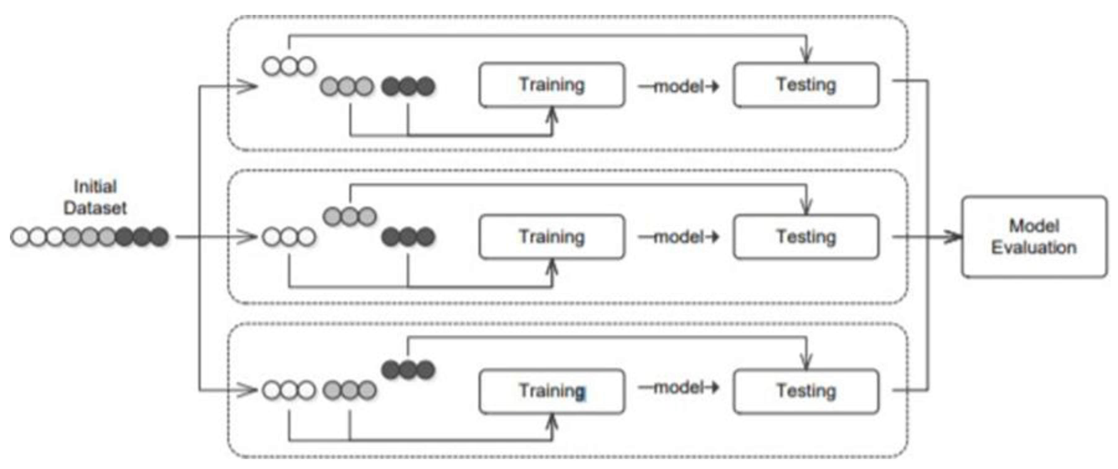
3. Methodology
3.1. Logistic Regression Model
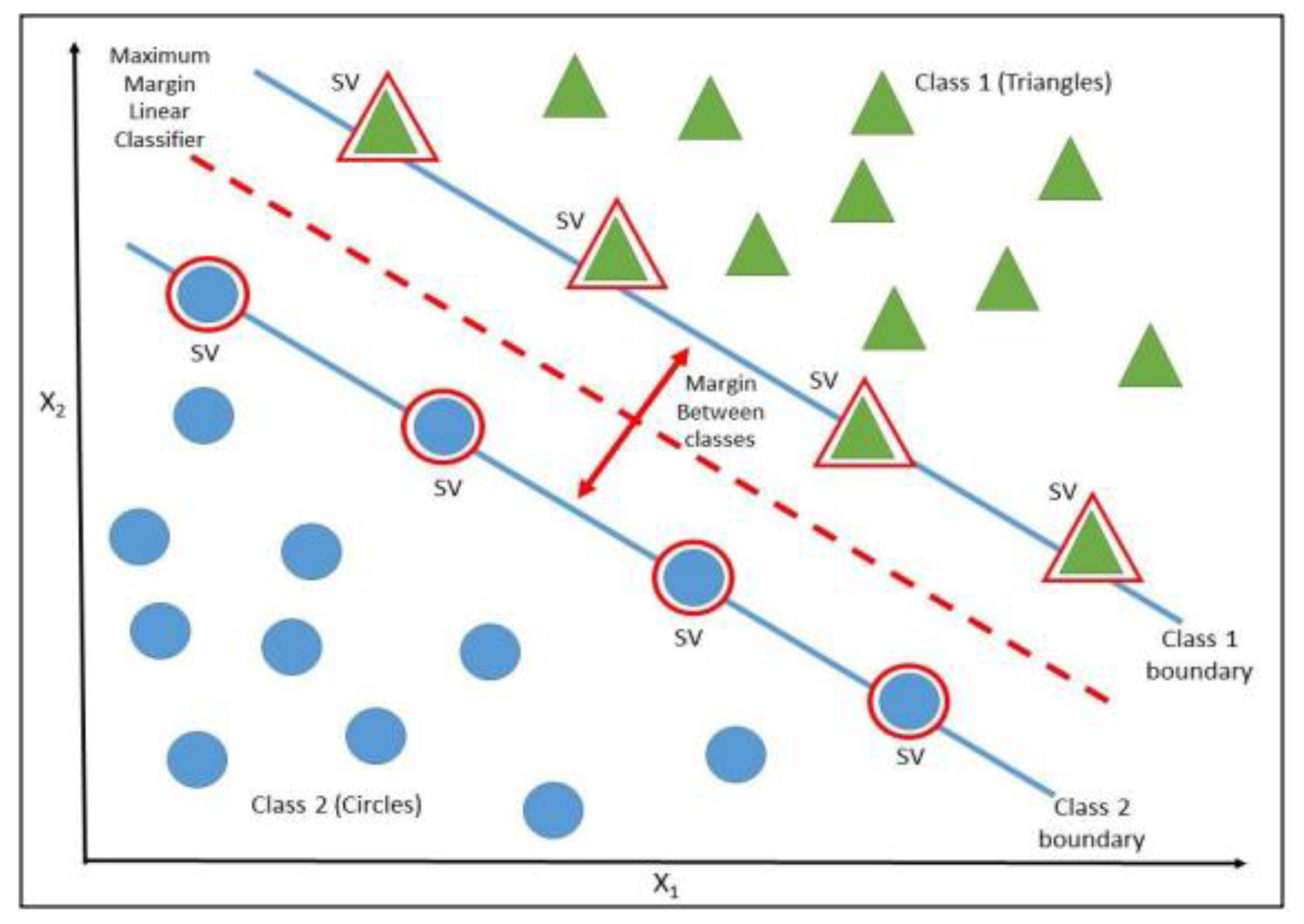
3.2. Support Vector Machine
3.3. Random Forests
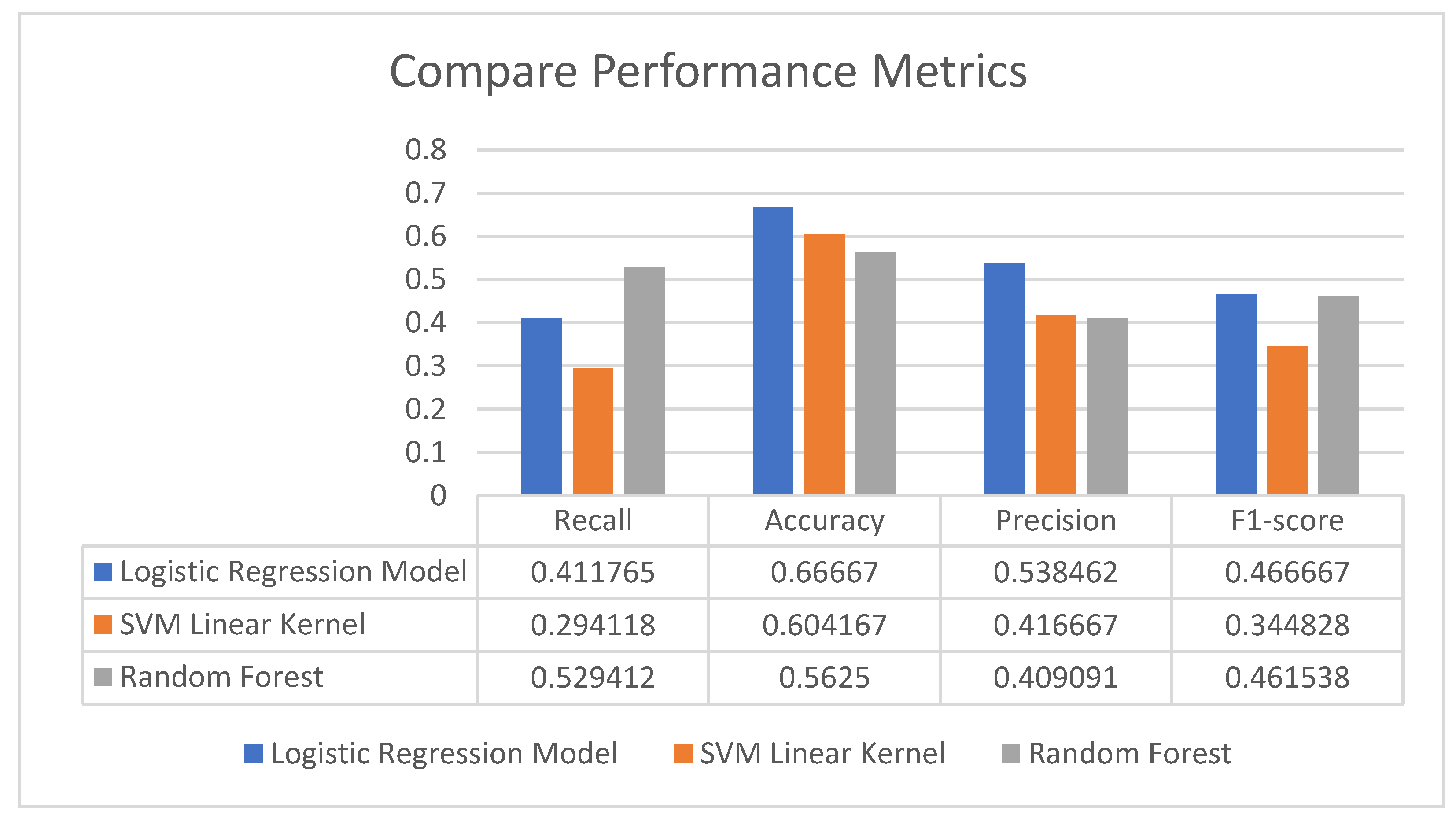
3.4. Performance Matrix
4. Empirical Results
5. Conclusions
Author Contributions
Funding
Conflicts of Interest
References
- Henriques, I.; Sadorsky, P. Can Bitcoin Replace Gold in an Investment Portfolio? J. Risk Financ. Manag. 2018, 11, 48. [Google Scholar] [CrossRef]
- Junttila, J.; Pesonen, J.; Raatikainen, J. Commodity market based hedging against stock market risk in times of financial crisis: The case of crude oil and gold. J. Int. Financ. Mark. Inst. Money 2018, 56, 255–280. [Google Scholar] [CrossRef]
- Tronzano, M. Financial Crises, Macroeconomic Variables, and Long-Run Risk: An Econometric Analysis of Stock Returns Correlations (2000 to 2019). J. Risk Financ. Manag. 2021, 14, 127. [Google Scholar] [CrossRef]
- Ferreira, M.; Rodrigues, S.; Reis, C.I.; Maximiano, M. Blockchain: A Tale of Two Applications. Appl. Sci. 2018, 8, 1506. [Google Scholar] [CrossRef]
- Fama, E.F. Efficient Capital Markets: A Review of Theory and Empirical Work. J. Financ. 1970, 25, 383–417. [Google Scholar] [CrossRef]
- Corbet, S.; Larkin, C.; Lucey, B.; Meegan, A.; Yarovaya, L. Cryptocurrency reaction to FOMC Announcements: Evidence of heterogeneity based on blockchain stack position. J. Financ. Stab. 2020, 46, 100706. [Google Scholar] [CrossRef]
- Joo, M.H.; Nishikawa, Y.; Dandapani, K. Announcement effects in the cryptocurrency market. Appl. Econ. 2020, 52, 4794–4808. [Google Scholar] [CrossRef]
- Basher, S.A.; Sadorsky, P. Forecasting Bitcoin price direction with random forests: How important are interest rates, inflation, and market volatility? Mach. Learn. Appl. 2022, 9, 100355. [Google Scholar] [CrossRef]
- Adcock, R.; Gradojevic, N. Non-fundamental, non-parametric Bitcoin forecasting. Phys. A Stat. Mech. Its Appl. 2019, 531, 121727. [Google Scholar] [CrossRef]
- Nakano, M.; Takahashi, A.; Takahashi, S. Bitcoin technical trading with artificial neural network. Phys. A Stat. Mech. Its Appl. 2018, 510, 587–609. [Google Scholar] [CrossRef]
- Jang, H.; Lee, J. An Empirical Study on Modeling and Prediction of Bitcoin Prices with Bayesian Neural Networks Based on Blockchain Information. IEEE Access 2018, 6, 5427–5437. [Google Scholar] [CrossRef]
- Lahmiri, S.; Bekiros, S. Cryptocurrency forecasting with deep learning chaotic neural networks. Chaos Solitons Fractals 2019, 118, 35–40. [Google Scholar] [CrossRef]
- Jain, A.; Tripathi, S.; Dwivedi, H.D.; Saxena, P. Forecasting Price of Cryptocurrencies Using Tweets Sentiment Analysis. In Proceedings of the 2018 Eleventh International Conference on Contemporary Computing (IC3), Noida, India, 2–4 August 2018; pp. 1–7. [Google Scholar] [CrossRef]
- Kraaijeveld, O.; De Smedt, J. The predictive power of public Twitter sentiment for forecasting cryptocurrency prices. J. Int. Financ. Mark. Inst. Money 2020, 65, 101188. [Google Scholar] [CrossRef]
- Valencia, F.; Gómez-Espinosa, A.; Valdés-Aguirre, B. Price Movement Prediction of Cryptocurrencies Using Sentiment Analysis and Machine Learning. Entropy 2019, 21, 589. [Google Scholar] [CrossRef]
- Corbet, S.; Larkin, C.; Lucey, B.M.; Meegan, A.; Yarovaya, L. The impact of macroeconomic news on Bitcoin returns. Eur. J. Financ. 2020, 26, 1396–1416. [Google Scholar] [CrossRef]
- Akyildirim, E.; Goncu, A.; Sensoy, A. Prediction of cryptocurrency returns using machine learning. Ann. Oper. Res. 2021, 297, 3–36. [Google Scholar] [CrossRef]
- Jaquart, P.; Dann, D.; Weinhardt, C. Short-term bitcoin market prediction via machine learning. J. Financ. Data Sci. 2021, 7, 45–66. [Google Scholar] [CrossRef]
- Chen, Z.; Li, C.; Sun, W. Bitcoin price prediction using machine learning: An approach to sample dimension engineering. J. Comput. Appl. Math. 2020, 365, 112395. [Google Scholar] [CrossRef]
- Yen, K.-C.; Cheng, H.-P. Economic Policy Uncertainty and Cryptocurrency Volatility. Financ. Res. Lett. 2021, 38, 101428. [Google Scholar] [CrossRef]
- Zięba, D.; Kokoszczyński, R.; Śledziewska, K. Shock transmission in the cryptocurrency market. Is Bitcoin the most influential? Int. Rev. Financ. Anal. 2019, 64, 102–125. [Google Scholar] [CrossRef]
- Vapnik, V. The Nature of Statistical Learning Theory; Springer: New York, NY, USA, 1995. [Google Scholar]
- Mehta, P.; Bukov, M.; Wang, C.-H.; Day, A.G.; Richardson, C.; Fisher, C.K.; Schwab, D.J. A high-bias, low-variance introduction to Machine Learning for physicists. Phys. Rep. 2019, 810, 1–124. [Google Scholar] [CrossRef] [PubMed]
- Russo, D.; Zou, J. How Much Does Your Data Exploration Overfit? Controlling Bias via Information Usage. IEEE Trans. Inf. Theory 2020, 66, 302–323. [Google Scholar] [CrossRef]
- Breiman, L. Bagging predictors. Mach Learn. 1996, 24, 123–140. [Google Scholar] [CrossRef]
- Lang, L.; Tiancai, L.; Shan, A.; Xiangyan, T. An improved random forest algorithm and its application to wind pressure prediction. Int. J. Intell. Syst. 2021, 36, 4016–4032. [Google Scholar] [CrossRef]
- Mishina, Y.; Murata, R.; Yamauchi, Y.; Yamashita, T.; Fujiyoshi, H. Boosted Random Forest. IEICE Trans. Inf. Syst. 2015, 98, 1630–1636. [Google Scholar] [CrossRef]
- Fernández, J.C.; Carbonero, M.; Gutiérrez, P.A.; Hervás-Martínez, C. Multi-objective evolutionary optimization using the relationship between F1 and accuracy metrics in classification tasks. Appl. Intell. 2019, 49, 3447–3463. [Google Scholar] [CrossRef]
- Vujovic, Ž.Ð. Classification Model Evaluation Metrics. Int. J. Adv. Comput. Sci. Appl. 2021, 12, 599–606. [Google Scholar] [CrossRef]
- Valverde-Albacete, F.J.; Peláez-Moreno, C. 100% Classification Accuracy Considered Harmful: The Normalized Information Transfer Factor Explains the Accuracy Paradox. PLoS ONE 2014, 9, e84217. [Google Scholar] [CrossRef] [PubMed]


| Variables | Name | Std | Mean | Skew | Kurt |
|---|---|---|---|---|---|
| TARGET | Bitcoin | 0.491265 | 0.401674 | 0.403676 | −1.852619 |
| Panel A: Macroeconomic Variables | |||||
| USEPUINDXD | Economic Policy Uncertainty Index for United States | 44.333749 | 87.418201 | 1.409511 | 4.538997 |
| Panel B: Exchange Rates | |||||
| EUR/USD | EUR/USD | 0.045994 | 1.133789 | 0.455684 | −0.134286 |
| GBP/USD | GBP/USD | 0.106192 | 1.370556 | 0.548099 | −1.066357 |
| JPY/USD | JPY/USD | 0.000436 | 0.008880 | 0.010883 | −0.234481 |
| AUD/USD | AUD/USD | 0.031169 | 0.749203 | 0.203230 | −0.407285 |
| Panel C: Interest Rates | |||||
| TB3MS | 3-Month Treasury Bill Secondary Market Rate, Discount Basis | 44.33288 | 87.412762 | 1.409956 | 4.540290 |
| DFII10 | Market Yield on U.S. Treasury Securities at 10-Year Constant Maturity | 0.414795 | 2.325826 | 0.085033 | −0.639574 |
| Panel D: Cryptocurrencies | |||||
| BTC Real | Bitcoin Real Price | 3783.646 | 3371.3188 | 1.320277 | 1.466443 |
| DOGE | Dogecoin | 3781.398 | 3375.7582 | 1.320594 | 1.469247 |
| MAID | MaidSafeCoin | 0.197630 | 0.195004 | 1.814227 | −0.328242 |
| XRP | XRP | 0.349752 | 0.231999 | 3.025756 | 13.524215 |
| NVC | Novacoin | 1.998961 | 1.882093 | 1.768265 | 2.927803 |
| NMC | Namecoin | 0.937335 | 0.955977 | 2.516421 | 8.185247 |
| LTC | Litecoin | 60.35639 | 43.998117 | 2.018088 | 4.684777 |
| GLC | Goldcoin | 0.071203 | 0.053806 | 2.404576 | 7.640745 |
| DASH | Dash | 218.0163 | 142.67451 | 2.471539 | 6.954688 |
| DEM | Deutsche eMark | 0.000019 | 0.000009 | 3.678487 | 15.999390 |
| ABY | ArtByte | 0.005136 | 0.002809 | 3.464867 | 15.451262 |
| DIME | Dimecoin | 0.011868 | 0.009364 | 3.020989 | 10.973465 |
| ORB | Orbitcoin | 0.163214 | 0.139930 | 2.294509 | 6.639723 |
| GRS | Groestlcoin | 0.380965 | 0.246300 | 2.019766 | 4.325836 |
| Panel E: Momentum Variables | |||||
| MOM5 | Momentum 5-Days | 1.146598 | 0.246300 | 0.412184 | −0.195015 |
| MOM10 | Momentum 10-Days | 1.591595 | 3.979079 | 0.349793 | −0.117683 |
| ΜOΜ15 | Momentum 15-Days | 2.102353 | 6.016736 | 0.311525 | −0.487390 |
| Predicted Label | |||
|---|---|---|---|
| 0 | 1 | ||
| Actual | 0 | TN | FP |
| (True Negatives) | (False Positives) | ||
| 1 | FN | TP | |
| (False Negatives) | (True Positives) | ||
| Recall | Accuracy | Precision | F1-Score | |
|---|---|---|---|---|
| Logistic Regression Model | 0.411765 | 0.66667 | 0.538462 | 0.466667 |
| SVM Linear Kernel | 0.058824 | 0.583333 | 0.200000 | 0.090909 |
| Random Forest | 0.588235 | 0.583333 | 0.434783 | 0.500000 |
Disclaimer/Publisher’s Note: The statements, opinions and data contained in all publications are solely those of the individual author(s) and contributor(s) and not of MDPI and/or the editor(s). MDPI and/or the editor(s) disclaim responsibility for any injury to people or property resulting from any ideas, methods, instructions or products referred to in the content. |
© 2023 by the authors. Licensee MDPI, Basel, Switzerland. This article is an open access article distributed under the terms and conditions of the Creative Commons Attribution (CC BY) license (https://creativecommons.org/licenses/by/4.0/).
Share and Cite
Dimitriadou, A.; Gregoriou, A. Predicting Bitcoin Prices Using Machine Learning. Entropy 2023, 25, 777. https://doi.org/10.3390/e25050777
Dimitriadou A, Gregoriou A. Predicting Bitcoin Prices Using Machine Learning. Entropy. 2023; 25(5):777. https://doi.org/10.3390/e25050777
Chicago/Turabian StyleDimitriadou, Athanasia, and Andros Gregoriou. 2023. "Predicting Bitcoin Prices Using Machine Learning" Entropy 25, no. 5: 777. https://doi.org/10.3390/e25050777
APA StyleDimitriadou, A., & Gregoriou, A. (2023). Predicting Bitcoin Prices Using Machine Learning. Entropy, 25(5), 777. https://doi.org/10.3390/e25050777