
Source Acquisition Device Identification from Recorded Audio Based on Spatiotemporal Representation Learning with Multi-Attention Mechanisms


Abstract
1. Introduction
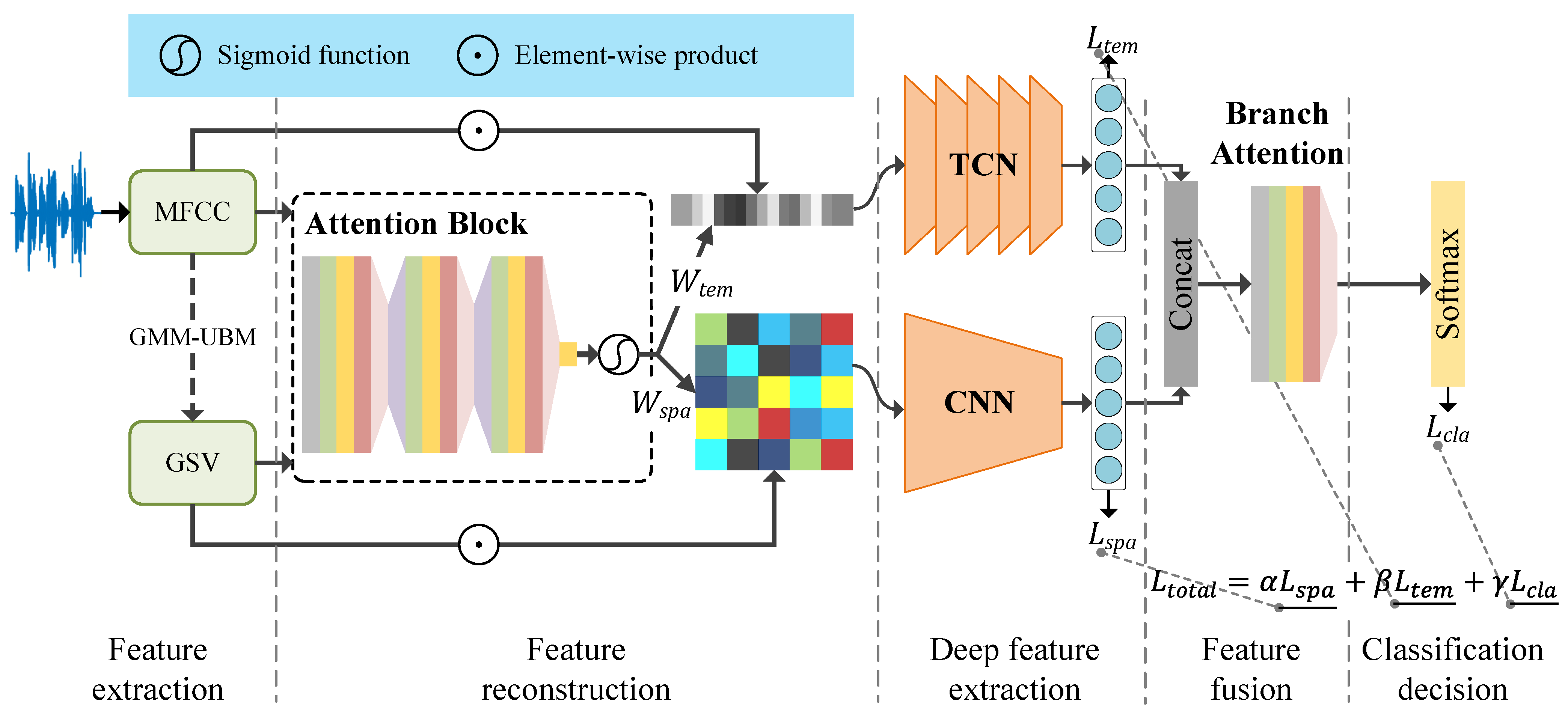
- In this paper, we propose a two-branch network to implement spatiotemporal representation learning for recording device identification. The extraction of deep temporal features is performed by a residual dense TCN, and the extraction of deep spatial features is performed by a CNN. The whole representation learning process is optimized by a structured loss function. The implementation codes of this research are available at https://github.com/CCNUZFW/STRLMA (accessed on 20 March 2023).
- In order to collaborate with the spatiotemporal representation network to obtain a better representation of recording devices, we design three attention mechanisms: a spatial attention mechanism, temporal attention mechanism, and branch attention mechanism. The spatial and temporal attention mechanisms assign weights to the input features Gaussian super vector (GSV) and MFCC, respectively, to enhance the representativeness of both features. The branch attention mechanism is applied to the fusion of two-way branches to promote the learning of key information in the fusion process.
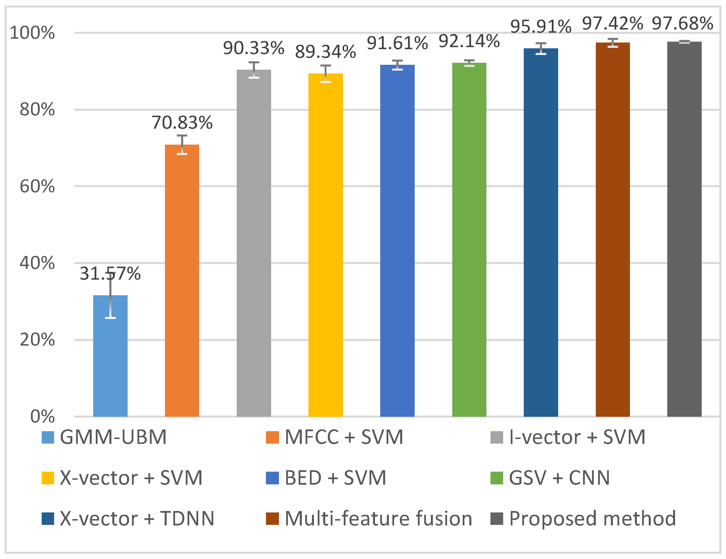
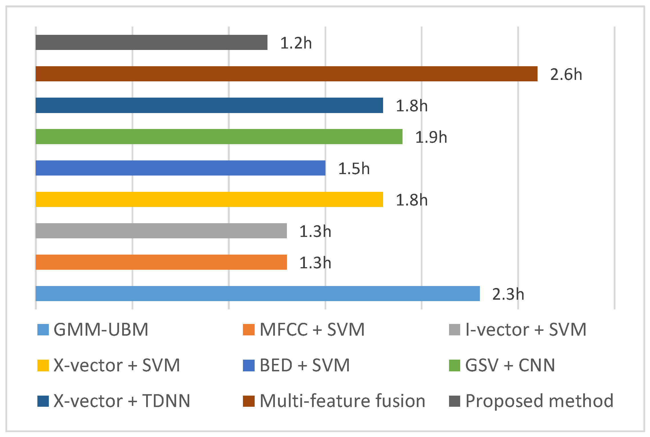
- Compared with six baseline methods, the proposed framework achieves state-of-the-art performance on the benchmark CCNU_Mobile dataset, reaching an accuracy of 97.6% for the identification of 45 recording devices, with a significant reduction in training time compared to baseline models.
2. Related Work
2.1. Recording Device Identification Based on Traditional Feature Engineering and Machine Learning
2.2. Recording Device Identification Based on Deep Learning
3. Preliminaries
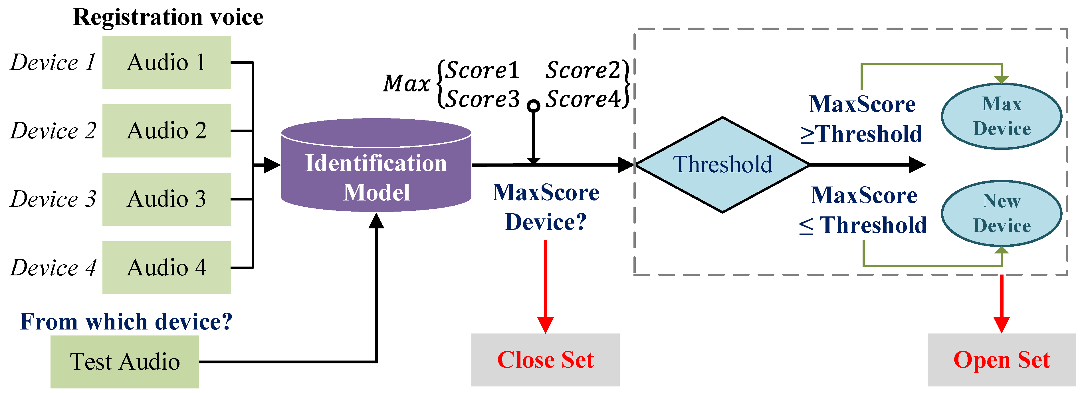
3.1. Problem Definition
3.2. Deep Feature and Multi-Attention Mechanism Definition
4. Methods
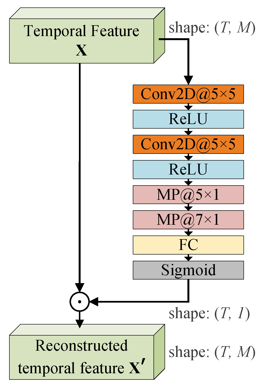
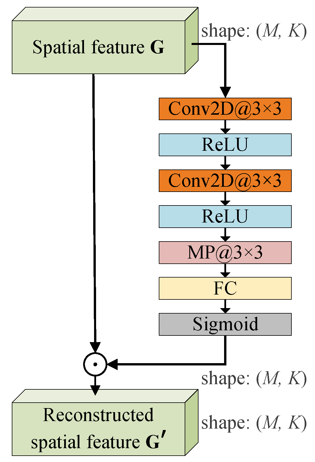
- The feature reconstruction phase is divided into temporal feature reconstruction and spatial feature reconstruction. Temporal feature reconstruction assigns adaptive weights to the features at the temporal scale through the attention mechanism and marks the significant sequences to improve the effects of important feature sequences on the model. Similarly, reconstruction for spatial information involves learning the spatial feature information using the attention mechanism to assign different weights to enhance spatial features.
- In the deep feature extraction stage, the temporal branch based on RD-TCN is used to extract the deep temporal features, and the spatial branch based on CNN is used to extract the deep spatial features.
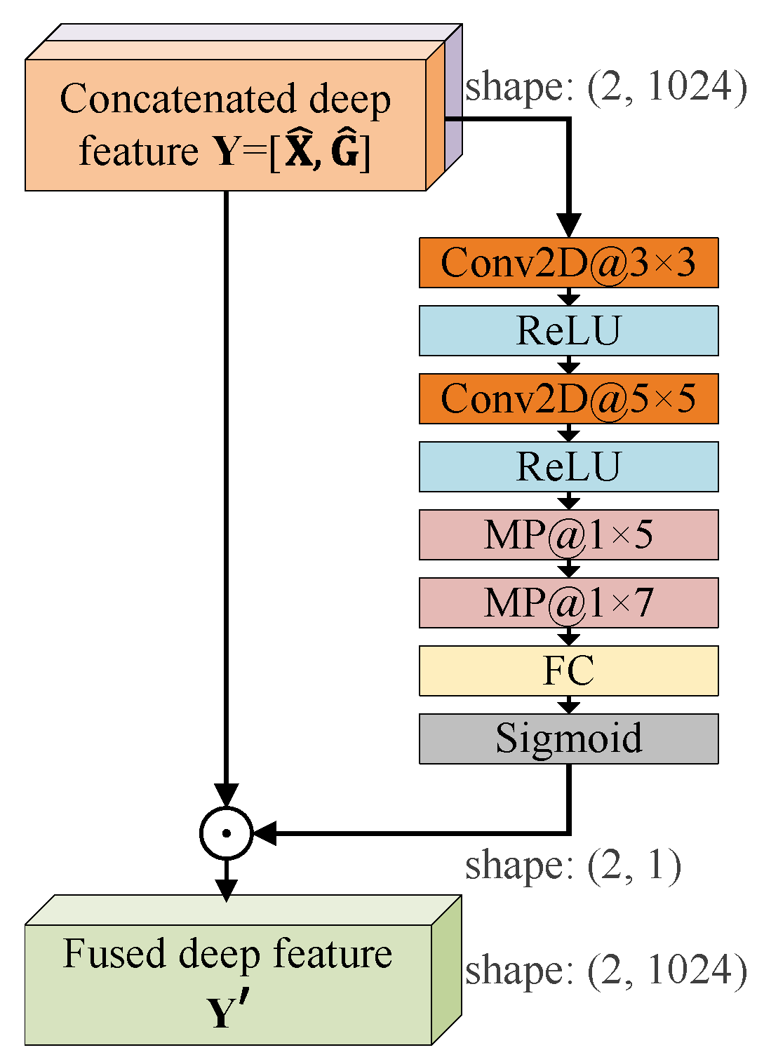
- In the feature fusion phase, a branch attention mechanism is designed for the fusion of deep temporal features and deep spatial features.
- In the classification decision phase, we apply a multiloss joint computation strategy in order to build an end-to-end network system and optimize the learning process of the two-way branch network and the decision end.
4.1. Feature Reconstruction Phase
4.1.1. Feature Reconstruction of MFCC Based on a Temporal Attention Mechanism
- First, in order to obtain a stable representation of the audio signal in the frequency domain, the audio signal () needs to be framed. A Hamming window with frame length () and frame shift () is used to obtain the short time frames;
- Then, the frequency spectral information of each frame is obtained by performing a fast Fourier transform on the framed and windowed signal;
- Then, Mel-scale triangular filters are used to filter the frequency spectra of frames;
- Then, the logarithmic amplitude spectrum at the output of each filter bank is calculated, and the M-dimension MFCC vectors are obtained by DCT calculation.
| Algorithm 1 The proposed spatiotemporal representation learning model. |
|
Input: MFCC feature : a sequence of MFCC vectors , GSV feature : a feature matrix of shape . Output: The prediction of the attributed recording device for the input sample 1 Reconstruct the input temporal feature into by temporal attention mechnism: 2 Reconstruct the input spatial feature into by spatial attention mechnism: 3 Extract deep spatial features through CNN blocks of spatial network branch: 4 Extract deep temporal features through RD-TCN blocks of the temporal network branch: 5 Compute spatial feature loss : 6 Compute temporal feature loss : 7 Concatenate deep temporal features and deep spatial features , and assign weights by branch attention mechanism to achieve feature fusion: 8 Compute classification loss : 9 Compute the overall loss : 10 Predict the source recording device . |
4.1.2. Feature Reconstruction of GSV Based on the Spatial Attention Mechanism
4.2. Deep Feature Extraction Phase
4.2.1. Deep Spatial Feature Extraction Based on CNN
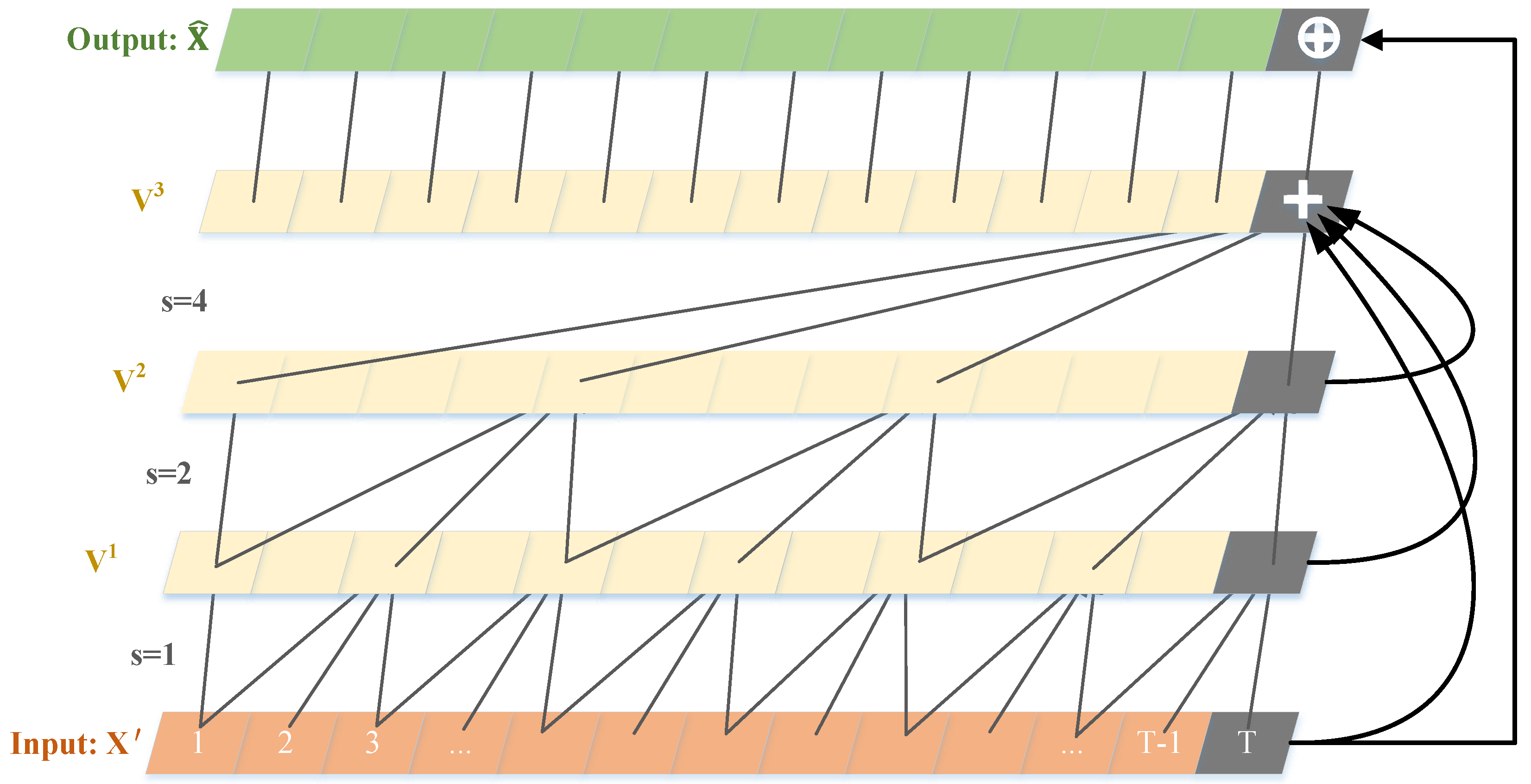
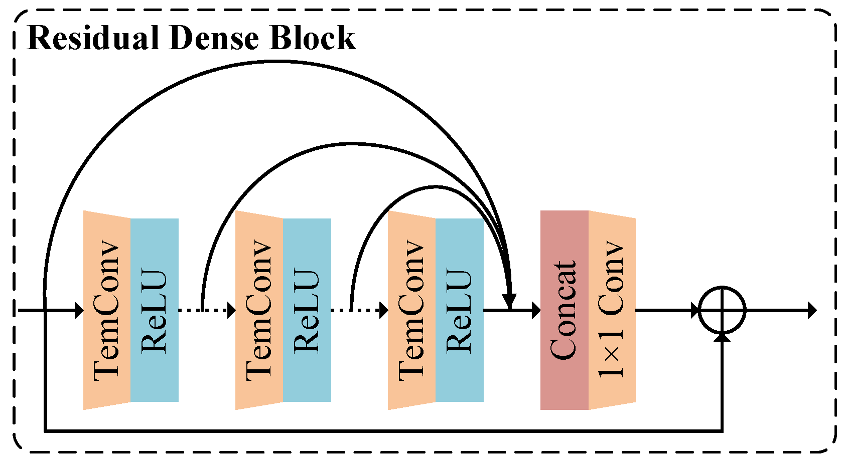
4.2.2. Deep Temporal Feature Extraction Based on RD-TCN
4.3. Feature Fusion Based on the Branch Attention Mechanism
4.4. Classification Decision Based on the Joint Loss Function
| Algorithm 2: Algorithm for model objective function learning |
 |
5. Experimental Results and Analysis
5.1. Dataset
5.2. Evaluation Metrics
5.3. Baselines
5.4. Experimental Settings
5.5. Results and Discussion
5.5.1. Comparison with Baseline Methods
5.5.2. Ablation Experiments of Attention Mechanisms
5.5.3. Validation Experiments of the RD-TCN Temporal Feature Extraction Network
5.5.4. Experiments for the Joint Loss Function
6. Conclusions
Author Contributions
Funding
Institutional Review Board Statement
Data Availability Statement
Conflicts of Interest
Abbreviations
| MFCC | Mel frequency cepstrum coefficient |
| BED | Band energy difference |
| VAD | Voice activity detection |
| SVM | Support vector machine |
| GMM | Gaussian mixture model |
| DNN | Deep neural network |
| GSV | Gaussian super vector |
| VQ | Vector quantization |
| SRC | Sparse representation-based classifier |
| 2D | Two-dimensional |
| FFT | Fast Fourier transform |
| DCT | Discrete cosine transform |
| EM | Expectation maximization |
| RNN | Recurrent neural network |
References
- Zeng, C.; Zhu, D.; Wang, Z.; Wang, Z.; Zhao, N.; He, L. An end-to-end deep source recording device identification system for Web media forensics. Int. J. Web Inf. Syst. 2020, 16, 413–425. [Google Scholar] [CrossRef]
- Maher, R.C. Audio forensic examination. IEEE Signal Process. Mag. 2009, 26, 84–94. [Google Scholar] [CrossRef]
- Wang, Z.; Yang, Y.; Zeng, C.; Kong, S.; Feng, S.; Zhao, N. Shallow and Deep Feature Fusion for Digital Audio Tampering Detection. EURASIP J. Adv. Signal Process. 2022, 2022, 69. [Google Scholar] [CrossRef]
- Zeng, C.; Yang, Y.; Wang, Z.; Kong, S.; Feng, S. Audio Tampering Forensics Based on Representation Learning of ENF Phase Sequence. Int. J. Digit. Crime Forensics 2022, 14, 94. [Google Scholar] [CrossRef]
- Luo, D.; Korus, P.; Huang, J. Band Energy Difference for Source Attribution in Audio Forensics. IEEE Trans. Inf. Forensics Secur. 2018, 13, 2179–2189. [Google Scholar] [CrossRef]
- Cuccovillo, L.; Aichroth, P. Open-set microphone classification via blind channel analysis. In Proceedings of the IEEE 2016 International Conference on Communications and Signal Processing (ICCSP), Shanghai, China, 20–25 March 2016; pp. 2074–2078. [Google Scholar] [CrossRef]
- Zhao, H.; Malik, H. Audio Recording Location Identification Using Acoustic Environment Signature. IEEE Trans. Inf. Forensics Secur. 2013, 8, 1746–1759. [Google Scholar] [CrossRef]
- Hanilci, C.; Ertas, F.; Ertas, T.; Eskidere, O. Recognition of Brand and Models of Cell-Phones from Recorded Speech Signals. IEEE Trans. Inf. Forensics Secur. 2012, 7, 625–634. [Google Scholar] [CrossRef]
- Hadoltikar, V.A.; Ratnaparkhe, V.R.; Kumar, R. Optimization of MFCC parameters for mobile phone recognition from audio recordings. In Proceedings of the IEEE 2019 3rd International Conference on Electronics, Communication and Aerospace Technology (ICECA), Coimbatore, India, 12–14 June 2019; pp. 777–780. [Google Scholar] [CrossRef]
- Hanilci, C.; Kinnunen, T. Source cell-phone recognition from recorded speech using non-speech segments. Digit. Signal Process. 2014, 35, 75–85. [Google Scholar] [CrossRef]
- Aggarwal, R.; Singh, S.; Roul, A.K.; Khanna, N. Cellphone identification using noise estimates from recorded audio. In Proceedings of the IEEE 2014 International Conference on Communications and Signal Processing (ICCSP), Melmaruvathur, India, 3–5 April 2014; pp. 1218–1222. [Google Scholar] [CrossRef]
- Kotropoulos, C.; Samaras, S. Mobile phone identification using recorded speech signals. In Proceedings of the IEEE 2014 International Conference on Digital Signal Processing (DSP), Hong Kong, China, 20–23 August 2014; pp. 586–591. [Google Scholar] [CrossRef]
- Jiang, Y.; Leung, F.H.F. Source Microphone Recognition Aided by a Kernel-Based Projection Method. IEEE Trans. Inf. Forensics Secur. 2019, 14, 2875–2886. [Google Scholar] [CrossRef]
- Garcia-Romero, D.; Espy-Wilson, C.Y. Automatic acquisition device identification from speech recordings. In Proceedings of the IEEE 2010 International Conference on Acoustics, Speech and Signal Processing, Dallas, TX, USA, 14–19 March 2010; pp. 1806–1809. [Google Scholar] [CrossRef]
- Li, Y.; Zhang, X.; Li, X.; Zhang, Y.; Yang, J.; He, Q. Mobile Phone Clustering from Speech Recordings Using Deep Representation and Spectral Clustering. IEEE Trans. Inf. Forensics Secur. 2018, 13, 965–977. [Google Scholar] [CrossRef]
- Qin, T.; Wang, R.; Yan, D.; Lin, L. Source Cell-Phone Identification in the Presence of Additive Noise from CQT Domain. Information 2018, 9, 205. [Google Scholar] [CrossRef]
- Baldini, G.; Amerini, I.; Gentile, C. Microphone Identification Using Convolutional Neural Networks. IEEE Sens. Lett. 2019, 3, 6001504. [Google Scholar] [CrossRef]
- Wang, S.; Cao, J.; Yu, P. Deep Learning for Spatio-Temporal Data Mining: A Survey. IEEE Trans. Knowl. Data Eng. 2020, 34, 3681–3700. [Google Scholar] [CrossRef]
- Lyu, L.; Wang, Z.; Yun, H.; Yang, Z.; Li, Y. Deep Knowledge Tracing Based on Spatial and Temporal Representation Learning for Learning Performance Prediction. Appl. Sci. 2022, 12, 7188. [Google Scholar] [CrossRef]
- Wu, Y.; Zhu, L.; Yan, Y.; Yang, Y. Dual Attention Matching for Audio-Visual Event Localization. In Proceedings of the 2019 IEEE/CVF International Conference on Computer Vision (ICCV), Seoul, Republic of Korea, 27 October–2 November 2019; pp. 6291–6299. [Google Scholar] [CrossRef]
- Campbell, W.M.; Sturim, D.E.; Reynolds, D.A. Support vector machines using GMM supervectors for speaker verification. IEEE Signal Process. Lett. 2006, 13, 308–311. [Google Scholar] [CrossRef]
- Reynolds, D.A. A mixture modeling approach to text-independent speaker ID. J. Acoust. Soc. Am. 1990, 87, S109. [Google Scholar] [CrossRef]
- Jin, C.; Wang, R.; Yan, D.; Tao, B.; Chen, Y.; Pei, A. Source Cell-Phone Identification Using Spectral Features of Device Self-noise. In Proceedings of the Digital Forensics and Watermarking: 15th International Workshop (IWDW), Beijing, China, 17–19 September 2016; pp. 29–45. [Google Scholar] [CrossRef]
- Wang, Z.; Zuo, C.; Zeng, C. SAE Based Unified Double JPEG Compression Detection System for Web Image Forensics. Int. J. Web Inf. Syst. 2021, 17, 84–98. [Google Scholar] [CrossRef]
- Zeng, C.; Ye, J.; Wang, Z.; Zhao, N.; Wu, M. Cascade Neural Network-Based Joint Sampling and Reconstruction for Image Compressed Sensing. Signal Image Video Process. 2022, 16, 47–54. [Google Scholar] [CrossRef]
- Wang, Z.; Wang, Z.; Zeng, C.; Yu, Y.; Wan, X. High-Quality Image Compressed Sensing and Reconstruction with Multi-Scale Dilated Convolutional Neural Network. Circuits Syst. Signal Process. 2023, 42, 1593–1616. [Google Scholar] [CrossRef]
- Zeng, C.; Yan, K.; Wang, Z.; Yu, Y.; Xia, S.; Zhao, N. Abs-CAM: A Gradient Optimization Interpretable Approach for Explanation of Convolutional Neural Networks. Signal Image Video Process. 2022, 1–8. [Google Scholar] [CrossRef]
- Li, Y.; Zhang, X.; Li, X.; Feng, X.; Yang, J.; Chen, A.; He, Q. Mobile phone clustering from acquired speech recordings using deep Gaussian supervector and spectral clustering. In Proceedings of the IEEE 2017 International Conference on Acoustics, Speech and Signal Processing (ICASSP), New Orleans, LA, USA, 5–9 March 2017; pp. 2137–2141. [Google Scholar] [CrossRef]
- Lin, X.; Zhu, J.; Chen, D. Subband Aware CNN for Cell-Phone Recognition. IEEE Signal Process. Lett. 2020, 27, 605–609. [Google Scholar] [CrossRef]
- Qi, S.; Huang, Z.; Li, Y.; Shi, S. Audio recording device identification based on deep learning. In Proceedings of the IEEE 2016 International Conference on Signal and Image Processing (ICSIP), Beijing, China, 13–15 August 2016; pp. 426–431. [Google Scholar] [CrossRef]
- Graves, A.; Mohamed, A.; Hinton, G. Speech recognition with deep recurrent neural networks. In Proceedings of the IEEE 2013 International Conference on Acoustics, Speech and Signal Processing (ICASSP), Vancouver, BC, Canada, 26–31 May 2013; pp. 6645–6649. [Google Scholar] [CrossRef]
- Zaremba, W.; Sutskever, I.; Vinyals, O. Recurrent neural network regularization. arXiv 2014, arXiv:1409.2329. [Google Scholar] [CrossRef]
- Zhang, Y.; Tian, Y.; Kong, Y.; Zhong, B.; Fu, Y. Residual dense network for image super-resolution. In Proceedings of the IEEE Conference on Computer Vision and Pattern Recognition (CVPR), Salt Lake City, UT, USA, 18–23 June 2018; pp. 2472–2481. [Google Scholar] [CrossRef]
- Rao, W.; Mak, M. Boosting the Performance of I-Vector Based Speaker Verification via Utterance Partitioning. IEEE Trans. Audio Speech Lang. Process. 2013, 21, 1012–1022. [Google Scholar] [CrossRef]
- Snyder, D.; Garcia-Romero, D.; Sell, G.; Povey, D.; Khudanpur, S. X-Vectors: Robust DNN Embeddings for Speaker Recognition. In Proceedings of the 2018 IEEE International Conference on Acoustics, Speech and Signal Processing (ICASSP), Calgary, AB, Canada, 15–20 April 2018; pp. 5329–5333. [Google Scholar] [CrossRef]
- Peddinti, V.; Povey, D.; Khudanpur, S. A time delay neural network architecture for efficient modeling of long temporal contexts. In Proceedings of the 16th Annual Conference of the International Speech Communication Association (Interspeech 2015), Dresden, Germany, 6–10 September 2015; pp. 3214–3218. [Google Scholar] [CrossRef]
- Yang, Y.; Zhuang, Y.; Pan, Y. Multiple knowledge representation for big data artificial intelligence: Framework, applications, and case studies. Front. Inf. Technol. Electron. Eng. 2021, 22, 1551–1558. [Google Scholar] [CrossRef]


| Notation | Description |
|---|---|
| Audio signal | |
| Frame length | |
| Frame shift | |
| MFCC features extracted after framing of samples | |
| K | Number of Gaussian components |
| GSV features of samples | |
| Convolution layer | |
| Maximum pooling layer | |
| Fully connected layer | |
| Sigmoid activation function | |
| ReLU activation function | |
| Weights | |
| Model parameters of GMM | |
| Components of the loss function | |
| Proportion coefficients of the three losses |
| Brand | Models |
|---|---|
| APPLE | iPhone6(4), iPhone6s(3), iPhone7p, iPhoneX, iPhoneSE, iPad7, Air1, Air2(2) |
| XIAOMI | mi2s, note3, mi5, mi8, mi8se(2), mix2, redmiNote4x, redmi3S |
| HUAWEI | Nova, Nova2s, Nova3e, P10, P20, TAG-AL00 |
| HONOR | honor7x, honor8(3), honorV8, honor9, honor10 |
| VIVO | x3f, x7, y11t |
| ZTE | C880a, G719c |
| SAMSUNG | S8, sphd710 |
| OPPO | R9s |
| NUBIA | Z11 |
| Spatial Attention Mechanism | Temporal Attention Mechanism | Branch Attention Mechanism |
|---|---|---|
| Conv(16, (3*3), (2*2)) | Conv (16, (5*5), (3*3)) | Conv (16, (3*3), (1*2)) |
| Conv(32, (3*3), (2*2)) | Conv (32, (3*3), (3*3)) | Conv (32, (5*5), (1*3)) |
| Pooling ((3*3), (2*2)) | Pooling ((5*1), (5*1)) | Pooling ((1*5), (1*5)) |
| Flatten | Pooling ((7*1), (7*1)) | Pooling ((1*7), (1*7)) |
| Dense (2496) | Flatten | Flatten |
| Reshape (39*64) | Dense (650) | Dense (2) |
| Multiply | Reshape (650*1) | Reshape (2*1) |
| / | Multiply | Multiply |
| Spatial Feature Extraction | Temporal Feature Extraction Network | |
|---|---|---|
| CNN | TCN Block | RD-TCN Block |
| Conv (6, (5*5), (1*1)) | Conv (6, 5, 1) | Conv (6, 5, 1) |
| Pooling ((2*2), (2*2)) | Conv (6, 5, 1) | Conv (6, 5, 1) |
| Conv (16, (5*5), (1*1)) | add | Conv (6, 5, 1) |
| Pooling ((2*2), (2*2)) | Conv (16, 5, 1) | add |
| Conv (40, (5*5), (1*1)) | Conv (16, 5, 1) | Conv (16, 5, 1) |
| Pooling ((2*2), (2*2)) | add | Conv (16, 5, 1) |
| Flatten | Conv (40, 3, 1) | Conv (16, 5, 1) |
| FC (1024) | Conv (40, 3, 1) | add |
| / | add | Conv (40, 3, 1) |
| / | / | Conv (40, 3, 1) |
| / | / | Conv (40, 3, 1) |
| / | / | add |
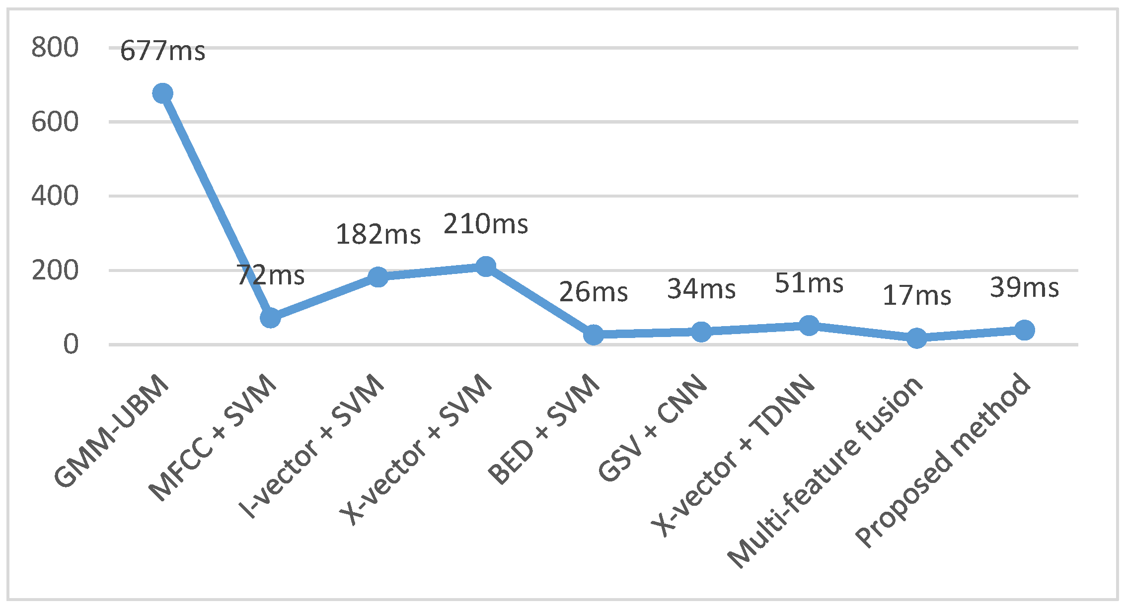
| Method | ACC | Training Time | Inference Time |
|---|---|---|---|
| GMM − UBM | 31.57 ± 11.65% | 2.3 h | 677 ms |
| MFCC + SVM | 70.83 ± 4.88% | 1.3 h | 72 ms |
| I-vector + SVM | 90.33 ± 3.93% | 1.3 h | 182 ms |
| X-vector + SVM | 89.34 ± 4.26% | 1.8 h | 210 ms |
| BED + SVM | 91.61 ± 2.41% | 1.5 h | 26 ms |
| GSV + CNN | 92.14 ± 1.40% | 1.9 h | 34 ms |
| X-vector + TDNN | 95.91 ± 2.76% | 1.8 h | 51 ms |
| Multifeature fusion | 97.42 ± 2.05% | 2.6 h | 17 ms |
| Proposed method | 97.68 ± 0.47% | 1.2 h | 39 ms |
| Model | ACC |
|---|---|
| Without temporal attention mechanism | 97.2% |
| Without spatial attention mechanism | 97.0% |
| Without branch attention mechanism | 97.2% |
| Model with three attention mechanisms | 97.6% |
| Model | ACC |
|---|---|
| Model with ordinary TCN block | 97.4% |
| Model with RD-TCN block | 97.6% |
| Loss Function Setting | Proportional Coefficients () | ACC |
|---|---|---|
| Single loss function | 0, 0, 1 | 96.7% |
| Joint loss function | 0.5, 0.25, 0.25 | 97.1% |
| Joint loss function | 0.25, 0.5, 0.25 | 97.6% |
| Joint loss function | 0.25, 0.25, 0.5 | 97.6% |
| Joint loss function | 0.4, 0.2, 0.4 | 97.3% |
| Joint loss function | 0.2, 0.6, 0.2 | 97.4% |
Disclaimer/Publisher’s Note: The statements, opinions and data contained in all publications are solely those of the individual author(s) and contributor(s) and not of MDPI and/or the editor(s). MDPI and/or the editor(s) disclaim responsibility for any injury to people or property resulting from any ideas, methods, instructions or products referred to in the content. |
© 2023 by the authors. Licensee MDPI, Basel, Switzerland. This article is an open access article distributed under the terms and conditions of the Creative Commons Attribution (CC BY) license (https://creativecommons.org/licenses/by/4.0/).
Share and Cite
Zeng, C.; Feng, S.; Zhu, D.; Wang, Z. Source Acquisition Device Identification from Recorded Audio Based on Spatiotemporal Representation Learning with Multi-Attention Mechanisms. Entropy 2023, 25, 626. https://doi.org/10.3390/e25040626
Zeng C, Feng S, Zhu D, Wang Z. Source Acquisition Device Identification from Recorded Audio Based on Spatiotemporal Representation Learning with Multi-Attention Mechanisms. Entropy. 2023; 25(4):626. https://doi.org/10.3390/e25040626
Chicago/Turabian StyleZeng, Chunyan, Shixiong Feng, Dongliang Zhu, and Zhifeng Wang. 2023. "Source Acquisition Device Identification from Recorded Audio Based on Spatiotemporal Representation Learning with Multi-Attention Mechanisms" Entropy 25, no. 4: 626. https://doi.org/10.3390/e25040626
APA StyleZeng, C., Feng, S., Zhu, D., & Wang, Z. (2023). Source Acquisition Device Identification from Recorded Audio Based on Spatiotemporal Representation Learning with Multi-Attention Mechanisms. Entropy, 25(4), 626. https://doi.org/10.3390/e25040626