
The Metastable State of Fermi–Pasta–Ulam–Tsingou Models


Abstract
1. Introduction
2. Methods
2.1. Models
2.2. Numerical Methods
2.3. Spectral Entropy
3. Phenomena
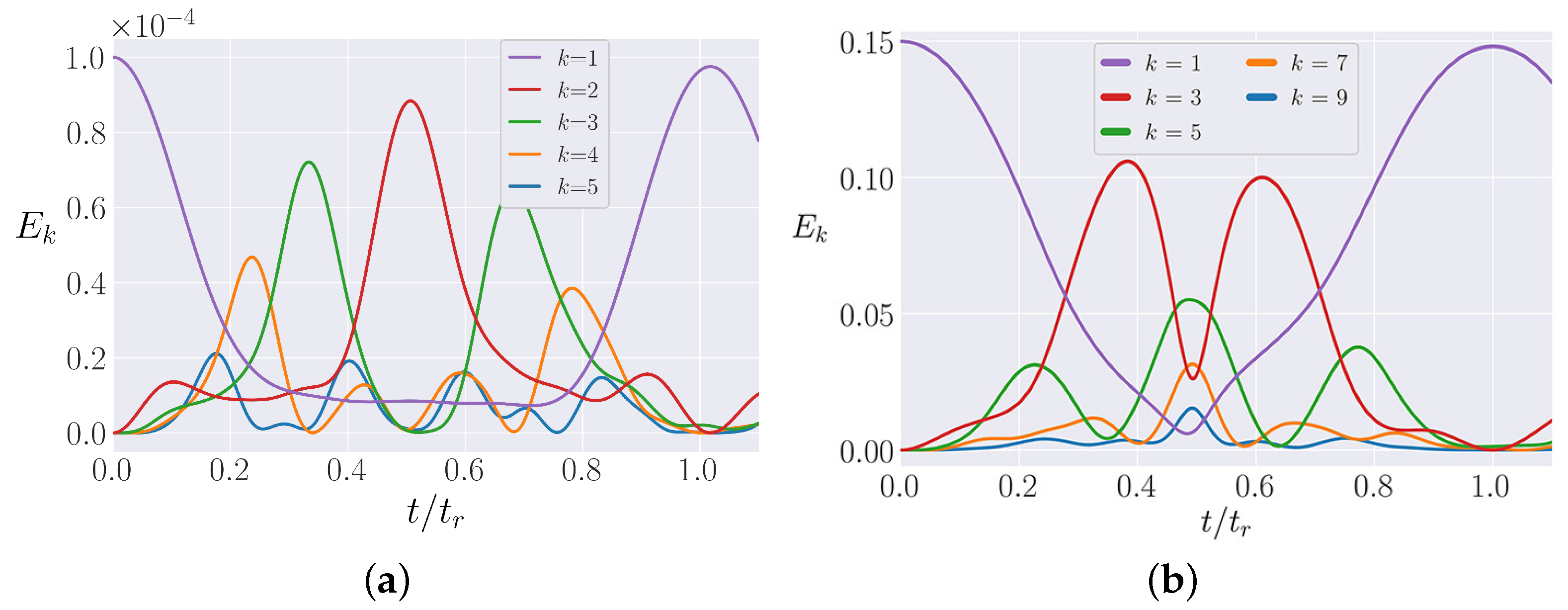
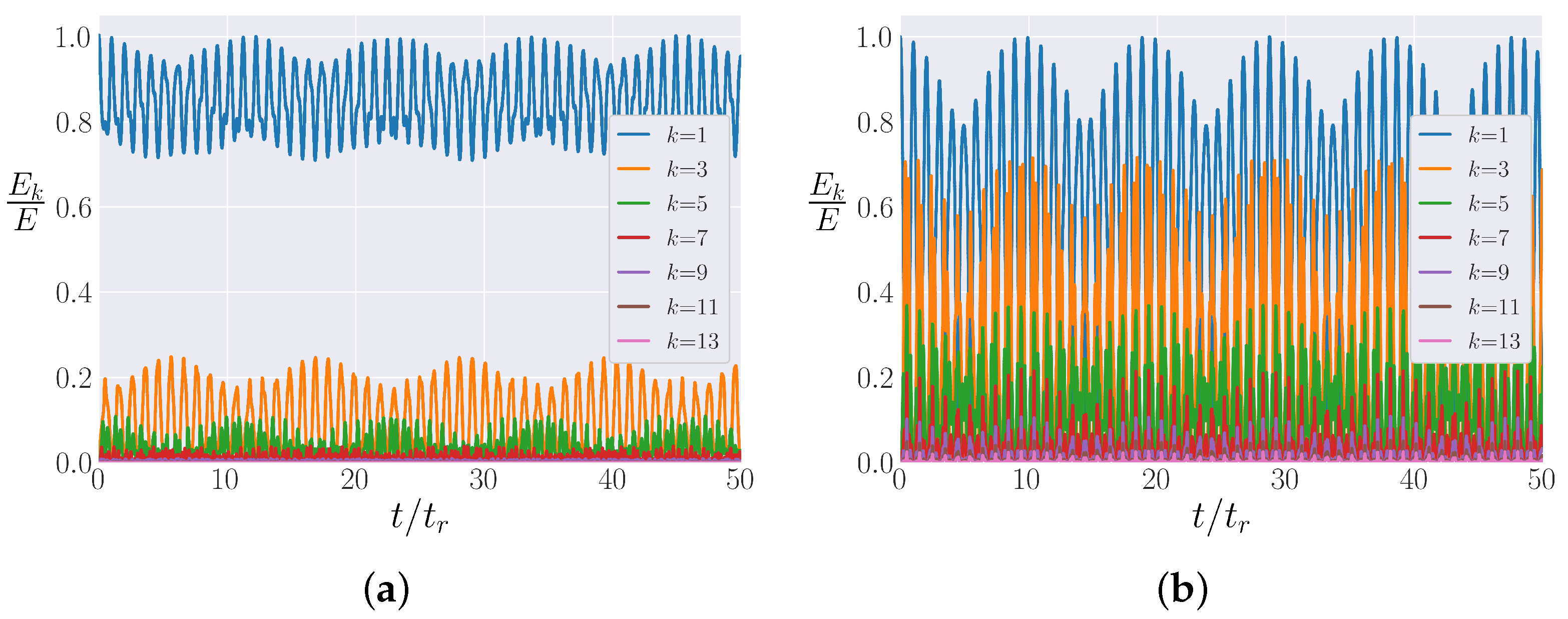
3.1. FPUT Recurrences
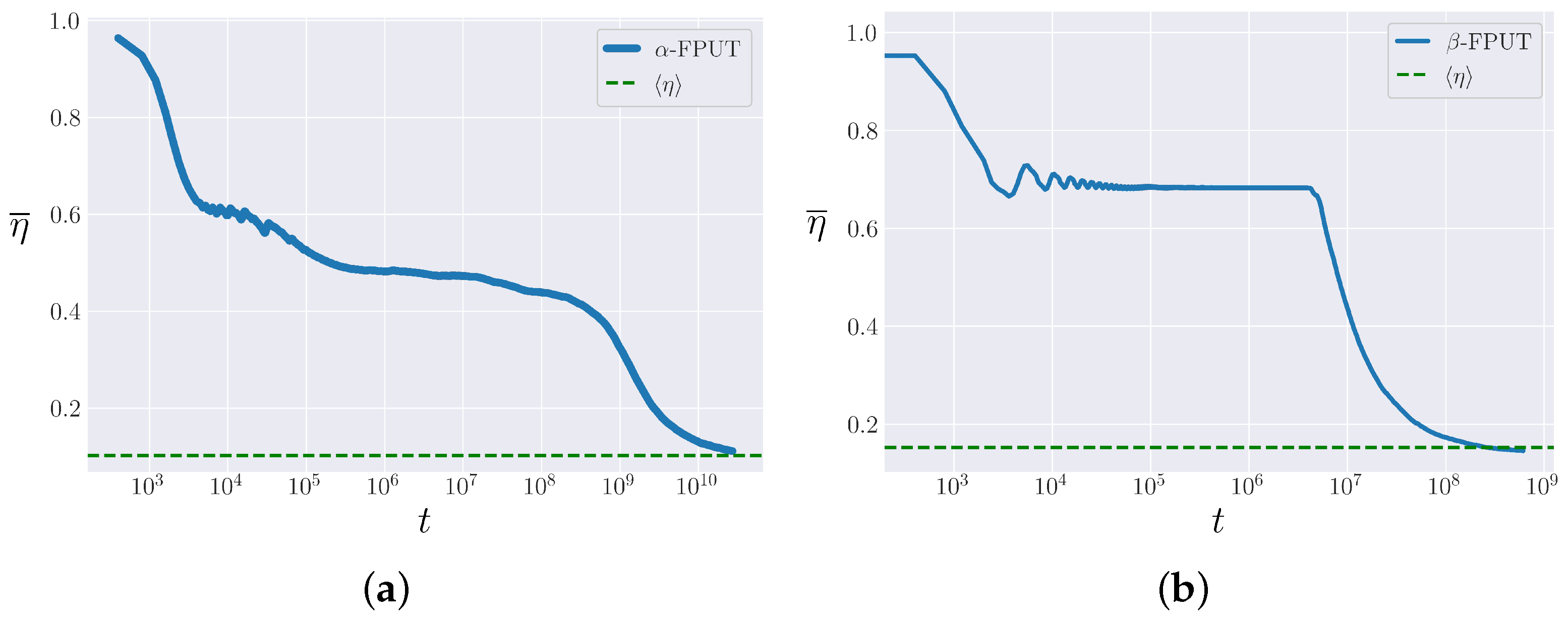
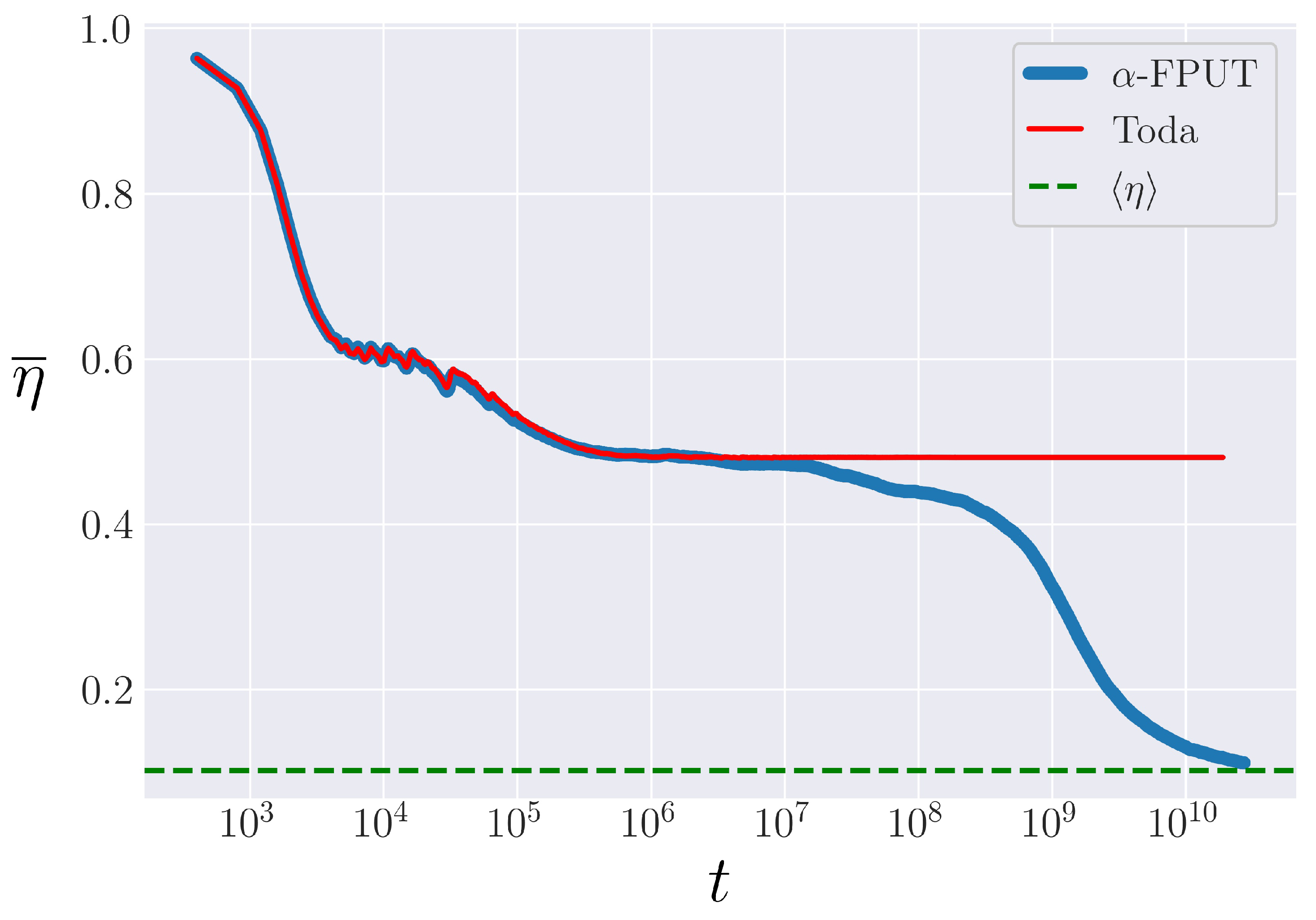
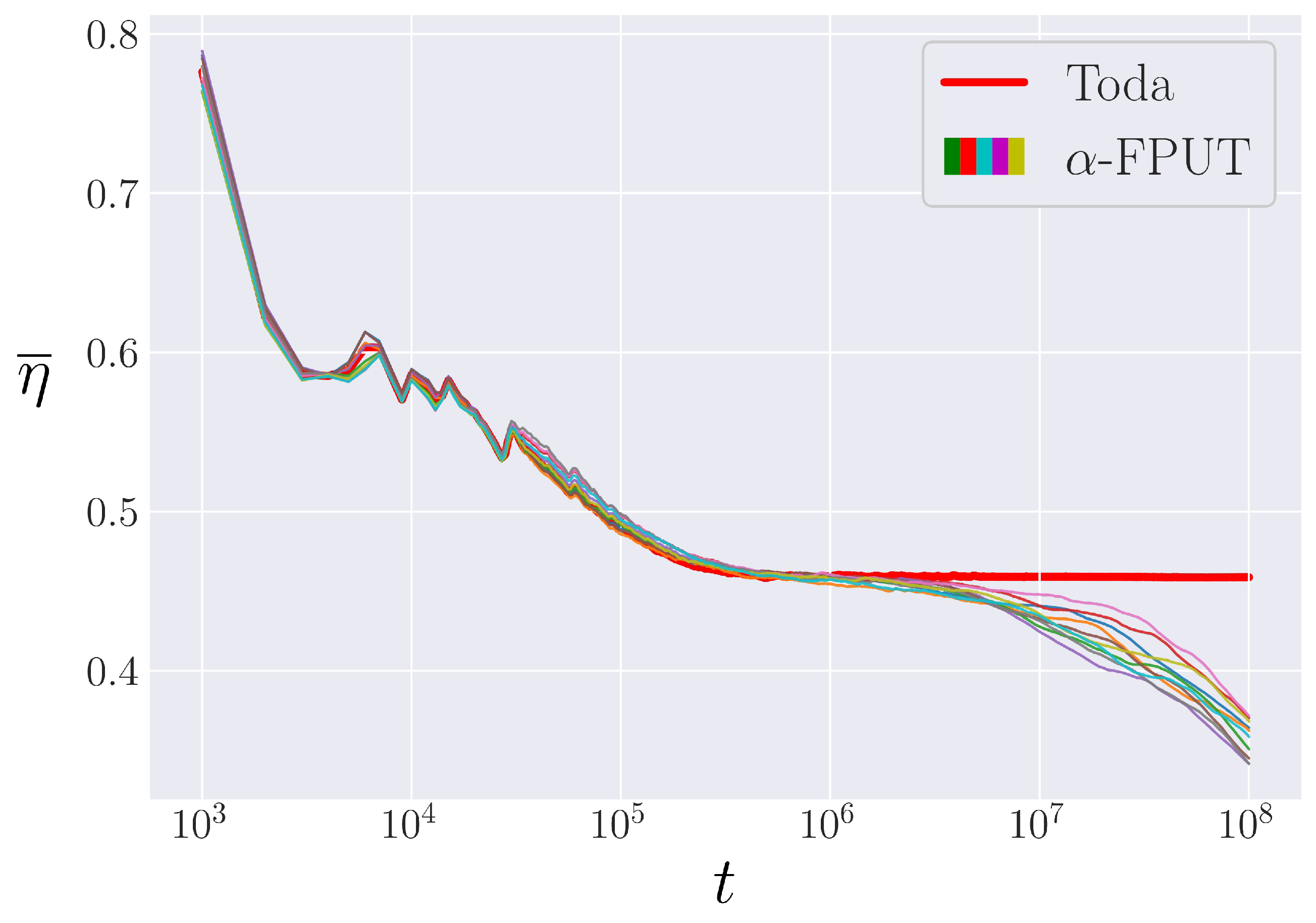
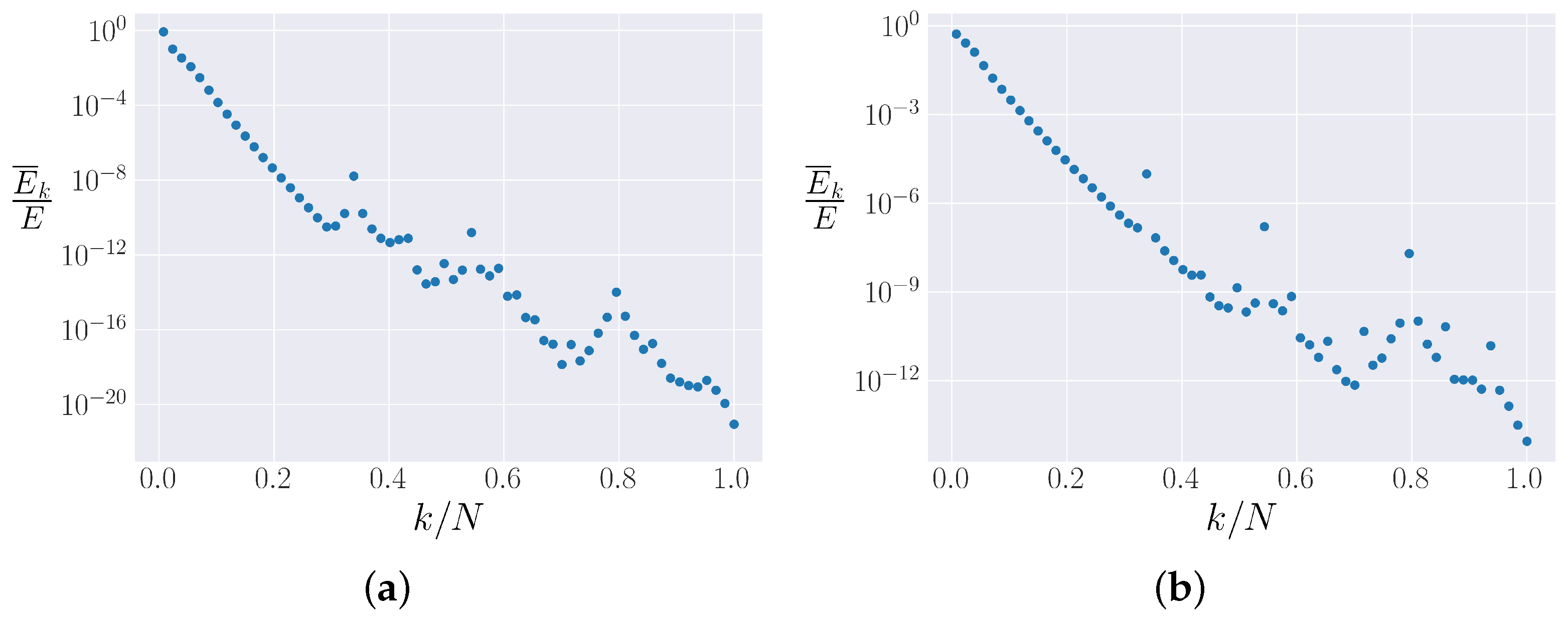
3.2. Metastable State
4. -FPUT Model
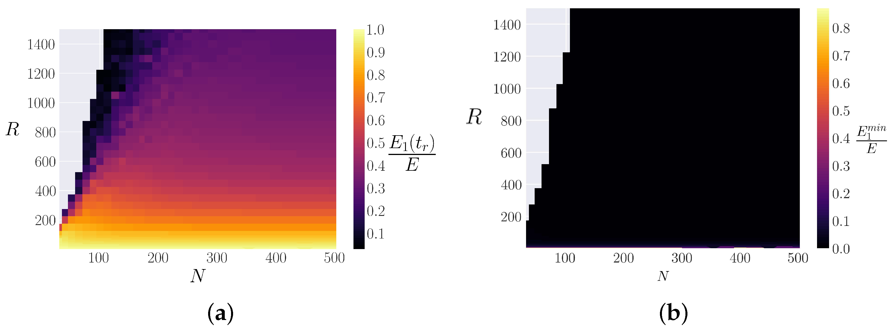
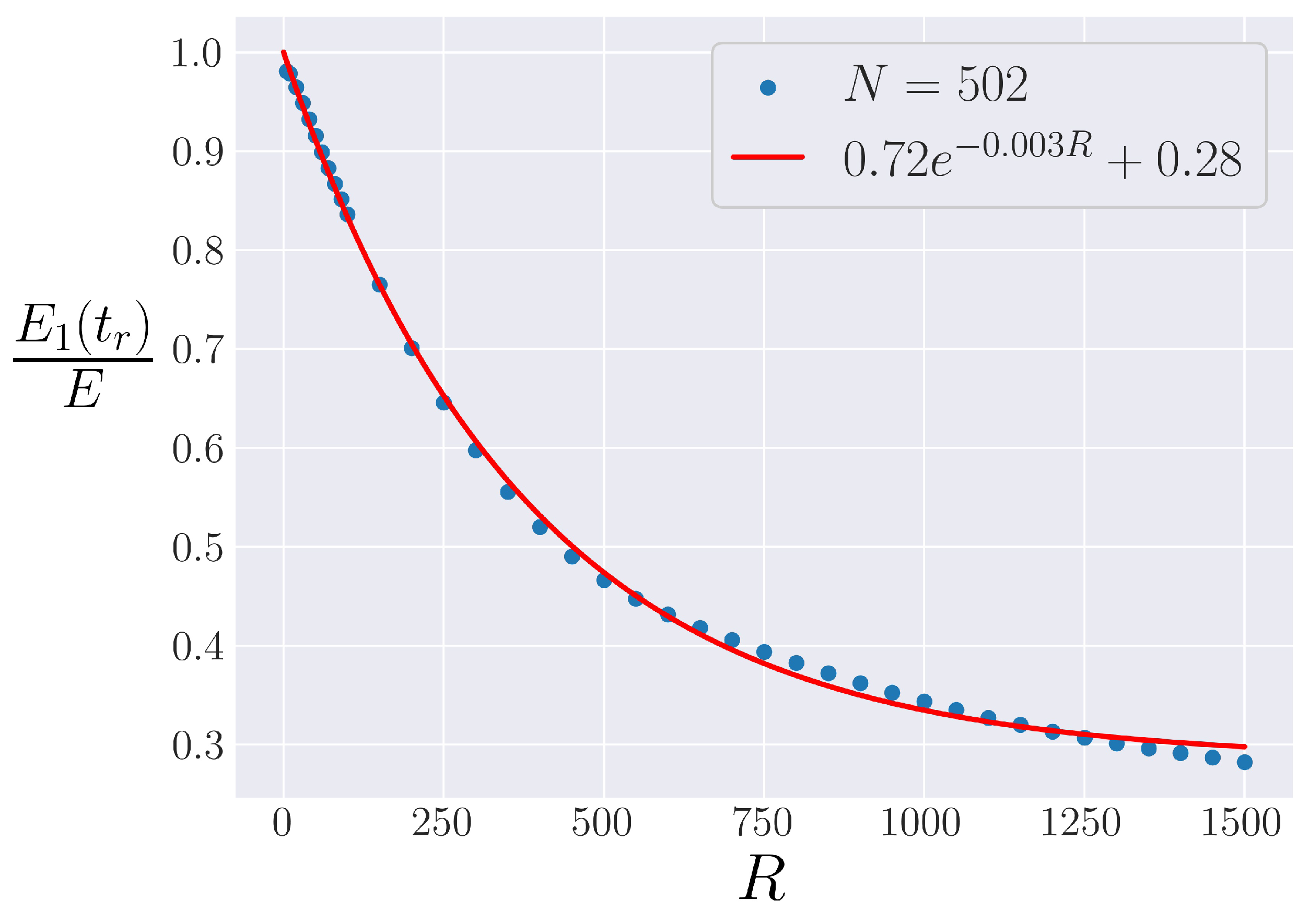
4.1. Strength of FPUT Recurrences
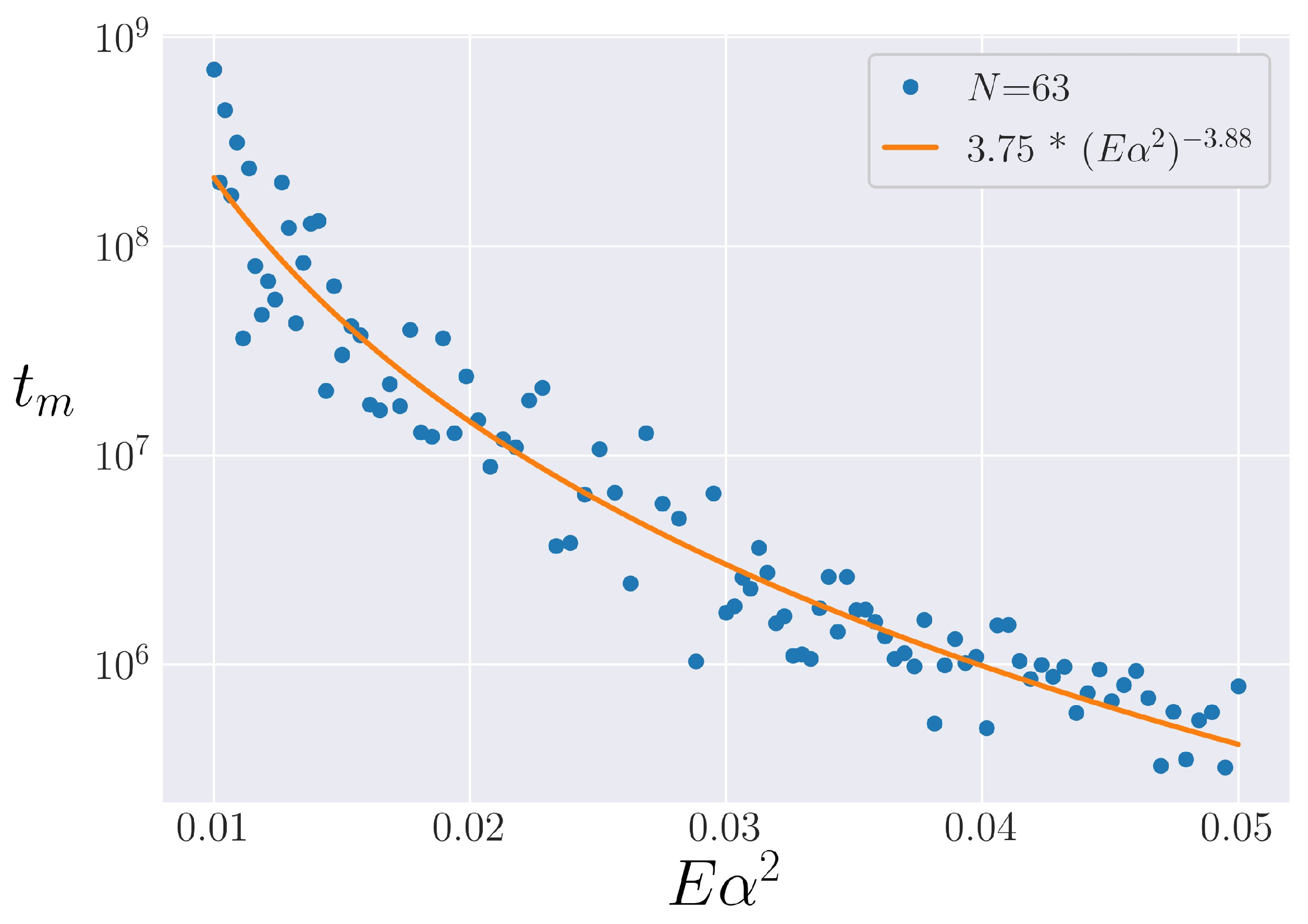
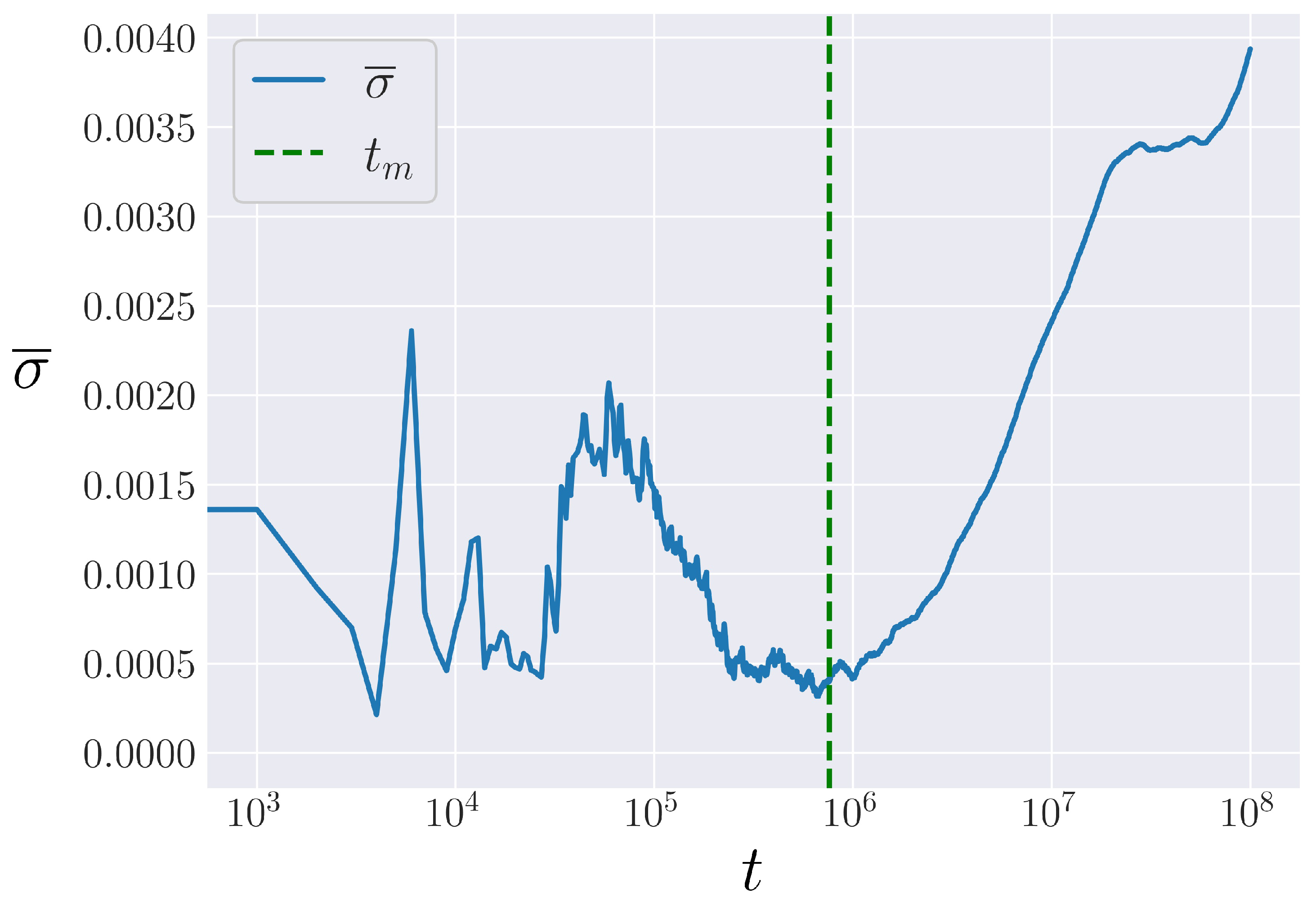
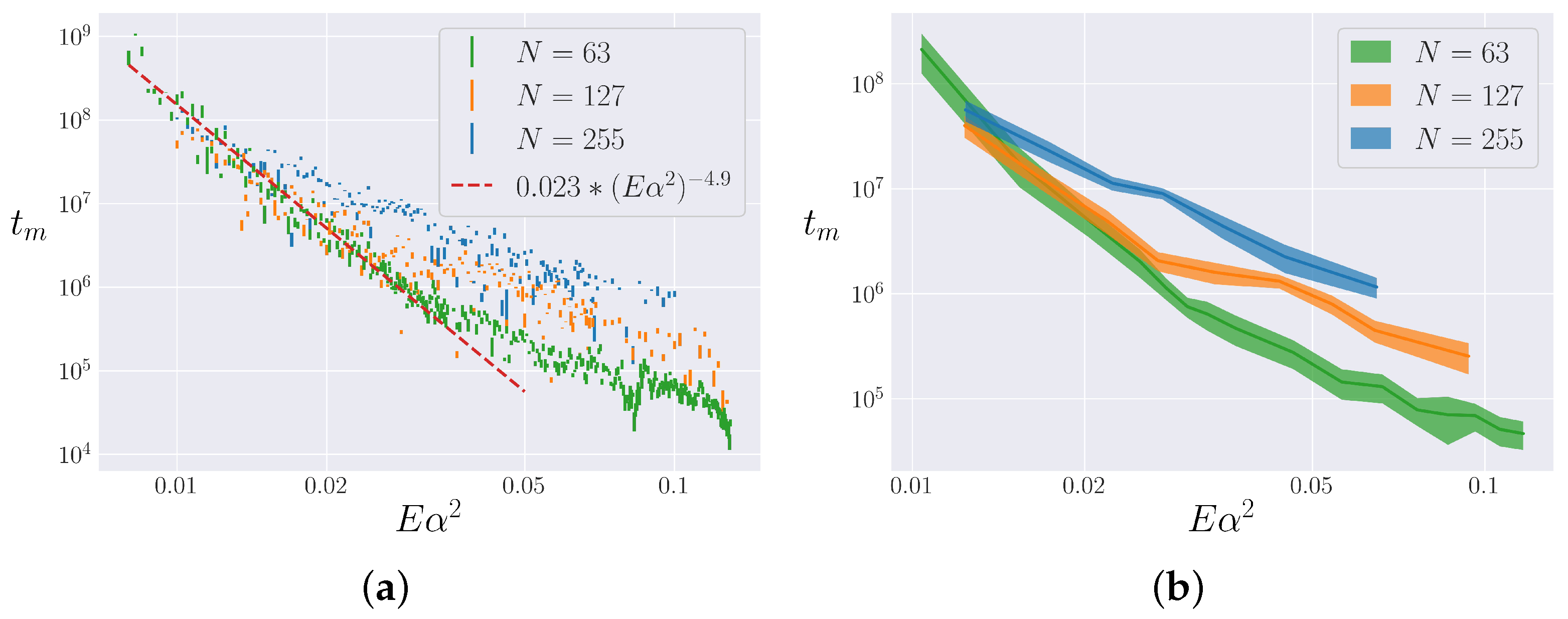
4.2. Lifetime of Metastable State
4.2.1. Procedure
4.2.2. Analysis
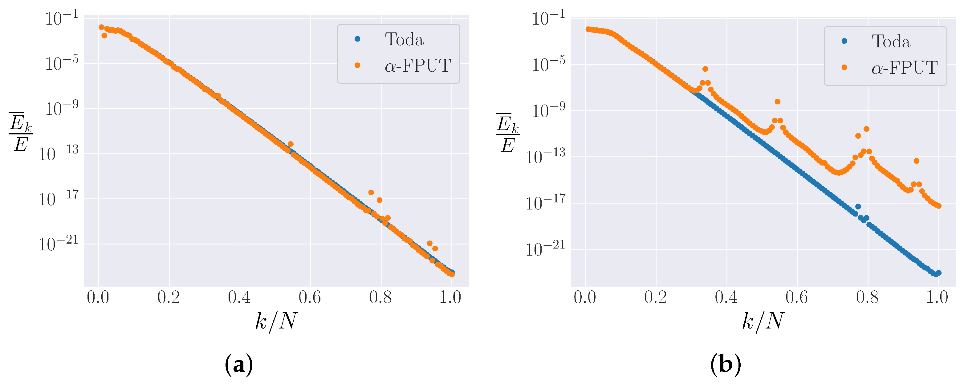
4.3. Spectrum
5. -FPUT Model
5.1. Comparison between and
5.2. Lifetime of Metastable State
6. Conclusions
Author Contributions
Funding
Institutional Review Board Statement
Data Availability Statement
Acknowledgments
Conflicts of Interest
References
- Pathria, R.K.; Beale, P.D. Statistical Mechanics, 3rd ed.; Elsevier: Amsterdam, The Netherlands, 2011. [Google Scholar] [CrossRef]
- Waterson, J.J. On the Physics of media that are composed of free and perfectly elastic molecules in a state of motion. R. Soc. 1851, 5, 604. [Google Scholar] [CrossRef]
- Thornton, S.T.; Rex, A.F. Modern Physics for Scientists and Engineers, 4th ed.; Cengage Learning: Boston, MA, USA, 2013. [Google Scholar]
- Wang, J.; Casati, G.; Benenti, G. Classical Physics and Blackbody Radiation. Phys. Rev. Lett. 2022, 128, 134101. [Google Scholar] [CrossRef]
- Fermi, E.; Pasta, J.R.; Ulam, S.; Tsingou, M. Studies of nonlinear problems, I. In Los Alamos Report; Los Alamos National Lab.(LANL): Los Alamos, NM, USA, 1955. [Google Scholar]
- Zabusky, N.J.; Kruskal, M.D. Interaction of “Solitons” in a Collisionless Plasma and the Recurrence of Initial States. Phys. Rev. Lett. 1965, 15, 240–243. [Google Scholar] [CrossRef]
- Flach, S.; Ivanchenko, M.V.; Kanakov, O.I. q-Breathers and the Fermi-Pasta-Ulam Problem. Phys. Rev. Lett. 2005, 95, 064102. [Google Scholar] [CrossRef]
- Campbell, D.K.; Rosenau, P.; Zaslavsky, G.M. Introduction: The Fermi–Pasta–Ulam problem—The first fifty years. Chaos Interdiscip. J. Nonlinear Sci. 2005, 15, 15101. [Google Scholar] [CrossRef] [PubMed]
- Gallavotti, G. (Ed.) The Fermi-Pasta-Ulam Problem: A Status Report; Number 728 in Lecture Notes in Physics; Springer: New York, NY, USA, 2008. [Google Scholar]
- Berman, G.P.; Izrailev, F.M. The Fermi–Pasta–Ulam problem: Fifty years of progress. Chaos: Interdiscip. J. Nonlinear Sci. 2005, 15, 15104. [Google Scholar] [CrossRef] [PubMed]
- Porter, M.; Zabusky, N.; Hu, B.; Campbell, D. Fermi, Pasta, Ulam and the Birth of Experimental Mathematics. Am. Sci. 2009, 97, 214. [Google Scholar] [CrossRef]
- Weissert, T.P. The Genesis of Simulation in Dynamics: Pursuing the Fermi-Pasta-Ulam Problem; Springer: New York, NY, USA, 1997. [Google Scholar]
- Benettin, G.; Carati, A.; Galgani, L.; Giorgilli, A. The fermi—pasta—ulam problem and the metastability perspective. In The Fermi-Pasta-Ulam Problem; Gallavotti, G., Ed.; Series Title: Lecture Notes in Physics; Springer: Berlin/Heidelberg, Germany, 2008; Volume 728, pp. 151–189. [Google Scholar] [CrossRef]
- Toda, M. Studies of a non-linear lattice. Phys. Rep. 1975, 18, 1–123. [Google Scholar] [CrossRef]
- Sholl, D. Modal coupling in one-dimensional anharmonic lattices. Phys. Lett. A 1990, 149, 253–257. [Google Scholar] [CrossRef]
- Bivins, R.; Metropolis, N.; Pasta, J.R. Nonlinear coupled oscillators: Modal equation approach. J. Comput. Phys. 1973, 12, 65–87. [Google Scholar] [CrossRef]
- Driscoll, C.F.; O’Neil, T.M. Explanation of Instabilities Observed on a Fermi-Pasta-Ulam Lattice. Phys. Rev. Lett. 1976, 37, 69–72. [Google Scholar] [CrossRef]
- Pace, S.D.; Campbell, D.K. Behavior and breakdown of higher-order Fermi-Pasta-Ulam-Tsingou recurrences. Chaos: Interdiscip. J. Nonlinear Sci. 2019, 29, 23132. [Google Scholar] [CrossRef]
- Driscoll, C.; O’Neil, T. Those ubiquitous, but oft unstable, lattice solitons. Rocky Mt. J. Math. 1978, 8, 211–225. [Google Scholar] [CrossRef]
- Danieli, C.; Many Manda, B.; Mithun, T.; Skokos, C. Computational efficiency of numerical integration methods for the tangent dynamics of many-body Hamiltonian systems in one and two spatial dimensions. Math. Eng. 2019, 1, 447–488. [Google Scholar] [CrossRef]
- Yoshida, H. Construction of higher order symplectic integrators. Phys. Lett. A 1990, 150, 262–268. [Google Scholar] [CrossRef]
- Shannon, C.E. A Mathematical Theory of Communication. Bell Syst. Tech. J. 1948, 27, 45. [Google Scholar] [CrossRef]
- Lin, C.; Goedde, C.; Lichter, S. Scaling of the recurrence time in the cubic Fermi-Pasta-Ulam lattice. Phys. Lett. A 1997, 229, 367–374. [Google Scholar] [CrossRef]
- Pace, S.D.; Reiss, K.A.; Campbell, D.K. The β Fermi-Pasta-Ulam-Tsingou recurrence problem. Chaos Interdiscip. J. Nonlinear Sci. 2019, 29, 113107. [Google Scholar] [CrossRef]
- Barreira, L. Poincaré recurrence: Old and new. In Proceedings of the XIVth International Congress on Mathematical Physics, Lisbon, Portugal, 28 July–2 August 2003; World Scientific: Lisbon, Portugal, 2006; pp. 415–422. [Google Scholar] [CrossRef]
- Danshita, I.; Hipolito, R.; Oganesyan, V.; Polkovnikov, A. Quantum damping of Fermi-Pasta-Ulam revivals in ultracold Bose gases. Prog. Theor. Exp. Phys. 2014, 2014, 43103. [Google Scholar] [CrossRef]
- Infeld, E. Quantitive Theory of the Fermi-Pasta-Ulam Recurrence in the Nonlinear Schrödinger Equation. Phys. Rev. Lett. 1981, 47, 717–718. [Google Scholar] [CrossRef]
- Kopidakis, G.; Soukoulis, C.M.; Economou, E.N. Electron-phonon interactions and recurrence phenomena in one-dimensional systems. Phys. Rev. B 1994, 49, 7036–7039. [Google Scholar] [CrossRef] [PubMed]
- Drago, G.; Ridella, S. Some more observations on the superperiod of the non-linear FPU system. Phys. Lett. A 1987, 122, 407–412. [Google Scholar] [CrossRef]
- Flach, S.; Ivanchenko, M.V.; Kanakov, O.I. q-breathers in Fermi-Pasta-Ulam chains: Existence, localization, and stability. Phys. Rev. E 2006, 73, 36618. [Google Scholar] [CrossRef]
- Christodoulidi, H.; Efthymiopoulos, C.; Bountis, T. Energy localization on q-tori, long-term stability, and the interpretation of Fermi-Pasta-Ulam recurrences. Phys. Rev. E 2010, 81, 016210. [Google Scholar] [CrossRef] [PubMed]
- Zabusky, J. Nonlinear Lattice Dynamics and Energy Sharing. J. Phys. Soc. Jpn. 1969, 26, 7. [Google Scholar]
- Fucito, F.; Marchesoni, F.; Marinari, E.; Parisi, G.; Peliti, L.; Ruffo, S.; Vulpiani, A. Approach to equilibrium in a chain of nonlinear oscillators. J. Phys. 1982, 43, 707–713. [Google Scholar] [CrossRef]
- Benettin, G.; Ponno, A. Time-Scales to Equipartition in the Fermi–Pasta–Ulam Problem: Finite-Size Effects and Thermodynamic Limit. J. Stat. Phys. 2011, 144, 793–812. [Google Scholar] [CrossRef]
- Benettin, G.; Christodoulidi, H.; Ponno, A. The Fermi-Pasta-Ulam Problem and Its Underlying Integrable Dynamics. J. Stat. Phys. 2013, 152, 195–212. [Google Scholar] [CrossRef]
- Benettin, G.; Pasquali, S.; Ponno, A. The Fermi–Pasta–Ulam Problem and Its Underlying Integrable Dynamics: An Approach Through Lyapunov Exponents. J. Stat. Phys. 2018, 171, 521–542. [Google Scholar] [CrossRef]
- Danieli, C.; Campbell, D.K.; Flach, S. Intermittent many-body dynamics at equilibrium. Phys. Rev. E 2017, 95, 60202. [Google Scholar] [CrossRef]
- Lin, C.Y.; Cho, S.N.; Goedde, C.G.; Lichter, S. When Is a One-Dimensional Lattice Small? Phys. Rev. Lett. 1999, 82, 4. [Google Scholar] [CrossRef]
- Ford, J. Equipartition of Energy for Nonlinear Systems. J. Math. Phys. 1961, 2, 387–393. [Google Scholar] [CrossRef]
- Ponno, A.; Christodoulidi, H.; Skokos, C.; Flach, S. The two-stage dynamics in the Fermi-Pasta-Ulam problem: From regular to diffusive behavior. Chaos Interdiscip. J. Nonlinear Sci. 2011, 21, 43127. [Google Scholar] [CrossRef] [PubMed]
- Onorato, M.; Vozella, L.; Proment, D.; Lvov, Y.V. Route to thermalization in the α-Fermi–Pasta–Ulam system. Proc. Natl. Acad. Sci. USA 2015, 112, 4208–4213. [Google Scholar] [CrossRef] [PubMed]


Disclaimer/Publisher’s Note: The statements, opinions and data contained in all publications are solely those of the individual author(s) and contributor(s) and not of MDPI and/or the editor(s). MDPI and/or the editor(s) disclaim responsibility for any injury to people or property resulting from any ideas, methods, instructions or products referred to in the content. |
© 2023 by the authors. Licensee MDPI, Basel, Switzerland. This article is an open access article distributed under the terms and conditions of the Creative Commons Attribution (CC BY) license (https://creativecommons.org/licenses/by/4.0/).
Share and Cite
Reiss, K.A.; Campbell, D.K. The Metastable State of Fermi–Pasta–Ulam–Tsingou Models. Entropy 2023, 25, 300. https://doi.org/10.3390/e25020300
Reiss KA, Campbell DK. The Metastable State of Fermi–Pasta–Ulam–Tsingou Models. Entropy. 2023; 25(2):300. https://doi.org/10.3390/e25020300
Chicago/Turabian StyleReiss, Kevin A., and David K. Campbell. 2023. "The Metastable State of Fermi–Pasta–Ulam–Tsingou Models" Entropy 25, no. 2: 300. https://doi.org/10.3390/e25020300
APA StyleReiss, K. A., & Campbell, D. K. (2023). The Metastable State of Fermi–Pasta–Ulam–Tsingou Models. Entropy, 25(2), 300. https://doi.org/10.3390/e25020300