1. Introduction
With the large-scale application of autonomous driving [
1], Intelligent Vehicles [
2], drone light formation show [
3], Internet-of-Things [
4] and other technologies, information technology is deeply integrated into our lives. As the foundation of information technology, wireless communication is easy to be affected by user interference and malicious jamming due to the openness of its channel, which reduces the efficiency of its actual deployment [
5,
6,
7,
8].
Addressing the impact of such issues is crucial in wireless communication systems [
9]. Therefore, making timely and effective spectrum decisions for different jamming patterns is practical in the anti-jamming process of wireless communication systems. Researchers have proposed various anti-jamming methods, including the extensively studied intelligent anti-jamming technology based on machine learning.
Table 1 shows a summary of related research, and mainly introduces the research status of intelligent anti-jamming technology based on federated learning (FL), meta-learning (Mate-L), reinforcement learning (RL), and deep reinforcement learning (DRL). To restore normal communication quickly and stably when the wireless communication system is faced with jamming, researchers use the method based on automatic control [
10,
11] to prevent jamming. To address the issue of local data secrecy during multi-agent anti-jamming communication, researchers employ federated learning (FL) [
12,
13,
14] for anti-jamming purposes. To enable agents to learn how to learn during anti-jamming communication, researchers have utilized meta-learning [
15,
16,
17] for anti-jamming. To facilitate anti-jamming decision-making as the state changes, researchers employ reinforcement learning (RL) [
18,
19,
20] for anti-jamming communication. To mitigate the “curse of dimensionality” problem associated with RL, researchers have extensively investigated the use of DQN [
21,
22,
23] for anti-jamming communication. DQN has shown promise in the field of anti-jamming decision-making due to its ability to make decisions while learning and adapting to new jamming scenarios. Building upon this foundation, scholars worldwide have proposed improved methods such as multi-agent layered Q-learning (MALQL) and UCB-DQN [
23].
The anti-jamming method based on automatic control can quickly and effectively deal with the current jamming and make appropriate anti-jamming actions, but this method cannot accumulate historical experience and cannot effectively predict the state change before anti-jamming. The intelligent anti-jamming communication methods are based on FL sacrifice performance for the sake of data security, and the performance is limited by the communication efficiency between agents. The intelligent anti-jamming communication method based on Meta-L requires high computing power, which is not practical for anti-jamming communication. The intelligent anti-jamming communication method based on RL fails to address the problem of continuous-state space and faces the challenge of the exponential growth of “state-action” pairs, known as the “dimension disaster”. The intelligent anti-jamming communication methods based on DQN have low sampling efficiency for state samples and limited utilization of historical state information, which may result in considerable time required for convergence even in typical or similar jamming scenarios. Furthermore, DQN imposes high requirements on the neural network, and an inappropriate neural network can lead to instability in the intelligent anti-jamming communication system based on DQN.
In our previous work, we mainly studied the intelligent anti-jamming communication technology based on RL [
5,
24] and DQN [
25], improved some technical details, and combined these with UCB technology. However, in this process, we find that both RL and DQN are faced with the dilemma of exploration and utilization, which requires a lot of time to explore the environment, and the ability to explore the environment in the utilization stage is poor. If the interference style is switched at this time, the anti-jamming ability of the system will be more significantly affected. In practice, jammers often enhance the difficulty of jamming by switching jamming patterns or dynamically adapting parameters. Consequently, efficiently utilizing experience from typical or similar scenarios to make effective anti-jamming decisions has become a challenging problem. With the advancement of research on inverse reinforcement learning, the method of imitation learning [
26,
27,
28] can be employed to make timely and effective anti-jamming decisions in the face of typical and similar scenarios. Therefore, we can obtain an efficient spectral decision-making method by analyzing historical samples, and take it as an expert strategy(ES), to form an expert trajectory(ET). Using imitation learning neural network(ILNN), we can obtain a user strategy capable of making efficient decisions, to significantly improve the response speed and robustness of decision-making. Unlike reinforcement learning, which needs to maintain a Q-table or DQN so that each state-action has its corresponding Q-value, the imitation learning method proposed in this paper treats the decision problem as a fitting problem of state-to-action selection probability. ILNN fits the action selection probability in the next time slot according to the state of several past moments. The system selects the anti-jamming action according to the selection probability. Therefore, there is no fear of the curse of dimensionality.
Based on this view, this manuscript proposes the following spectrum anti-jamming method using IL for scenarios where varied conventional jamming appears alternatively:
First, a proposed Expert Trajectory Generation Algorithm (ETGA) serves as the expert strategy. Anti-jamming decision-making is carried out on historical state samples (HSS). To enable the system to stably avoid jamming signals, the expert strategy is generated accordingly.
Next, Imitation Learning Neural Networks are proposed. It takes historical state samples as input and the expert strategy generated by ETGA as expected output. Through network training, a user strategy (US) can be obtained, enabling it to make decisions according to the state of several previous time slots.
Finally, the user strategy is used as a function to obtain anti-jamming decision actions efficiently and sequentially based on the states of multiple previous timeslots in the anti-jamming process.
The remainder of this manuscript is organized as follows:
Section 2 introduces the system model and problem formulation.
Section 3 explains the method.
Section 4 presents the simulation results. Finally,
Section 5 summarizes the conclusions.
2. System Model and Problem Formulation
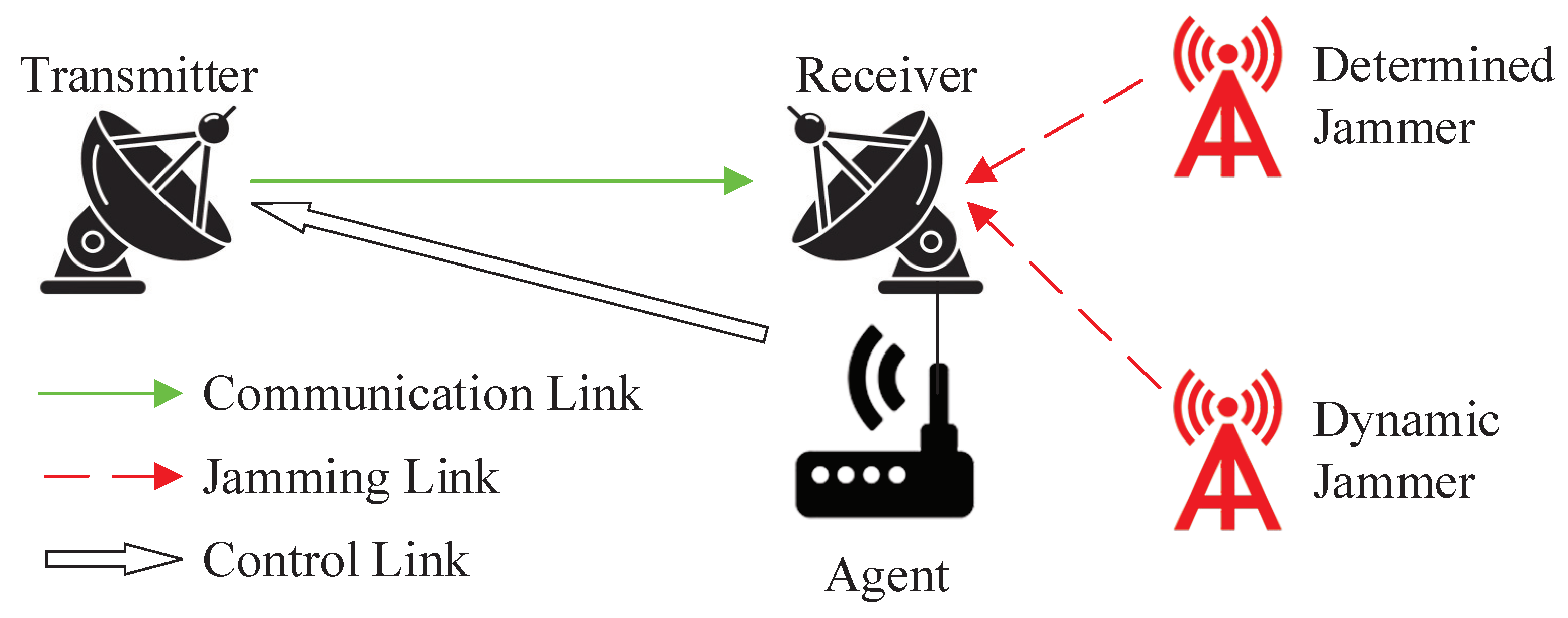
This section presents the system model and problem formulation of this manuscript. The system comprises a transmitter, receiver, agent, and jammer. The problem formulation introduces the reward function and objective function discussed in this manuscript.
2.1. System Model
The system model in this manuscript, depicted in
Figure 1, considers a wireless communication scenario where multiple malicious jammers are present. The transmitter
T sends the signal
while the receiver
R is being maliciously jammed by both the determined jammer and the dynamic jammer. The agent at the receiver perceives the state
, and learns and decides on the anti-jamming action
, and transmits it to the transmitter through an independent control link to modify the communication action [
5].
2.2. Problem Formulation
This subsection outlines the reward function and objective function for this problem. The reward function is dependent on the current state and the chosen action. The objective function aims to minimize the disparity between the reward obtained from the user strategy and the reward achieved from the expert strategy.
2.2.1. Reward Function
The communication band is divided into
N non-overlapping channels, and the state
is represented by a
array where each element corresponds to the strength of the noise plus jamming signal
of each channel:
Similarly, the action a is defined as a
array with only one element being 1 and the others being 0.
The reward
r obtained by selecting action
in state
is given by the following:
where
is the energy threshold for jamming plus noise.
2.2.2. Objective Function
To solve the anti-jamming problem, we use imitation learning to learn from the expert strategy and minimize the difference between the user reward expectation (URE) and the expert reward expectation (ERE) under policy .
IL aims to learn tasks from expert strategy, which can extract information about actions and the surrounding environment, and learn the relationship between states and actions.
For a given expert strategy
, the expert reward expectation can be calculated according to this strategy
. Generally speaking, expert strategy
is often manifested as expert strategy, that is, the action switching process under the expert strategy
. For
m expert strategies
the expert reward expectation
is calculated as follows:
At the same time, for the user who adopts user strategy
, its user reward expectation (URE) can be expressed as follows:
We expect the Agent to minimize the difference between the user reward expectation
and the expert reward expectation
under policy
:
3. Method
This section proposes an anti-jamming method using imitation learning based on the above system model for the system model in
Section 2. First, the process structure of the designed anti-jamming method using imitation learning is given, then the Expert Trajectory Generation Algorithm is given, and finally, the design of imitation learning neural network is given.
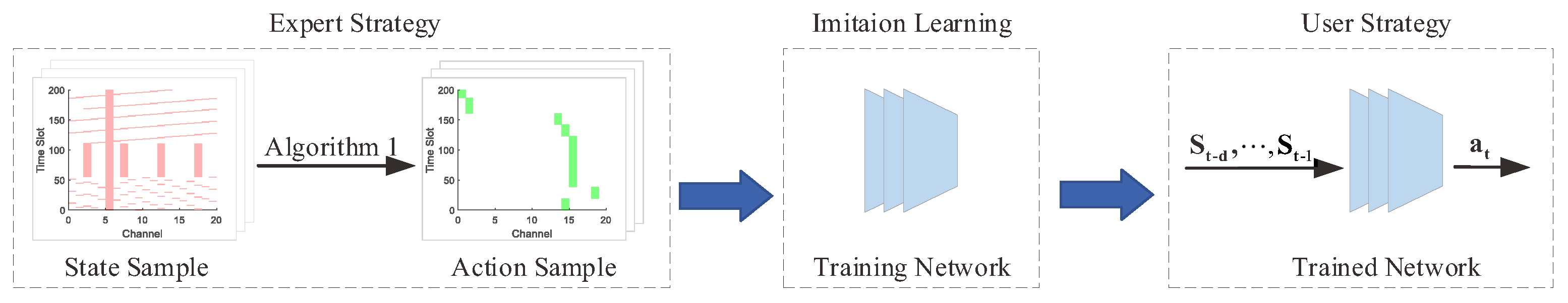
3.1. Process Structure
As illustrated in
Figure 2, the process structure of the designed anti-jamming method using imitation learning is proposed for intelligent spectrum anti-jamming in the scenario described in
Section 2.
The first step is to obtain the state sample
through the perception of the RF environment. The expert strategy
is then generated through the expert strategy, as shown in Algorithm 1,
The expert strategy is generated posteriorly, allowing the algorithm to select the action
based on either the state change before or after the timeslot, maximizing the total communication reward of this trajectory. The resulting expert strategy
can be expressed as
which is an action sequence equal to the length of the training sample
timeslot.
In anti-jamming practice, the network parameters
are adjusted through learning and adjusting to obtain the maximum reward by observing historical jamming information and obtaining the next action through the function
The ILNN is trained to imitate the expert strategy to obtain the user strategy, and the function
is used as the efficient decision function during the process, obtaining the next action
through the following formula:
Implementing this algorithm faces two challenges, which are addressed in the next section:
| Algorithm 1 Expert Trajectory Generation Algorithm (ETGA) |
Input: Time-frequency matrix RF (N*M). Output: Expert selection sequence ESS (1*M). initialize: ESS = zeros(1,M); Consecutive unjammed channel start timeslot S1 = 1; Consecutive unjammed channel end timeslot S2 = TL. while min(ESS) == 0 do J = zeros(N,1) for ii = 1:N do if sum(RF(ii,S1:S2) > 0) == 0 then J(ii) = S2+1; else J(ii) = find(RF(ii,S1:S2) > 0,1)+S1−1 end if end for [M,N] = max(J); ESS(S1:M−1) = N*ones(M−S1,1); S1 = M; end while
|
3.2. Expert Trajectory Generation Algorithm (ETGA)
The Expert Trajectory Generation Algorithm (ETGA) is shown in Algorithm 1. The algorithm selects the trajectory according to the time-frequency state matrix of based on the expert strategy, ensuring no collision with the jamming channel and that the communication signal stays in the same channel as long as possible for stable and sequential communication.
The expert strategy corresponding to the Expert selection sequence (ESS) in Algorithm 1 is
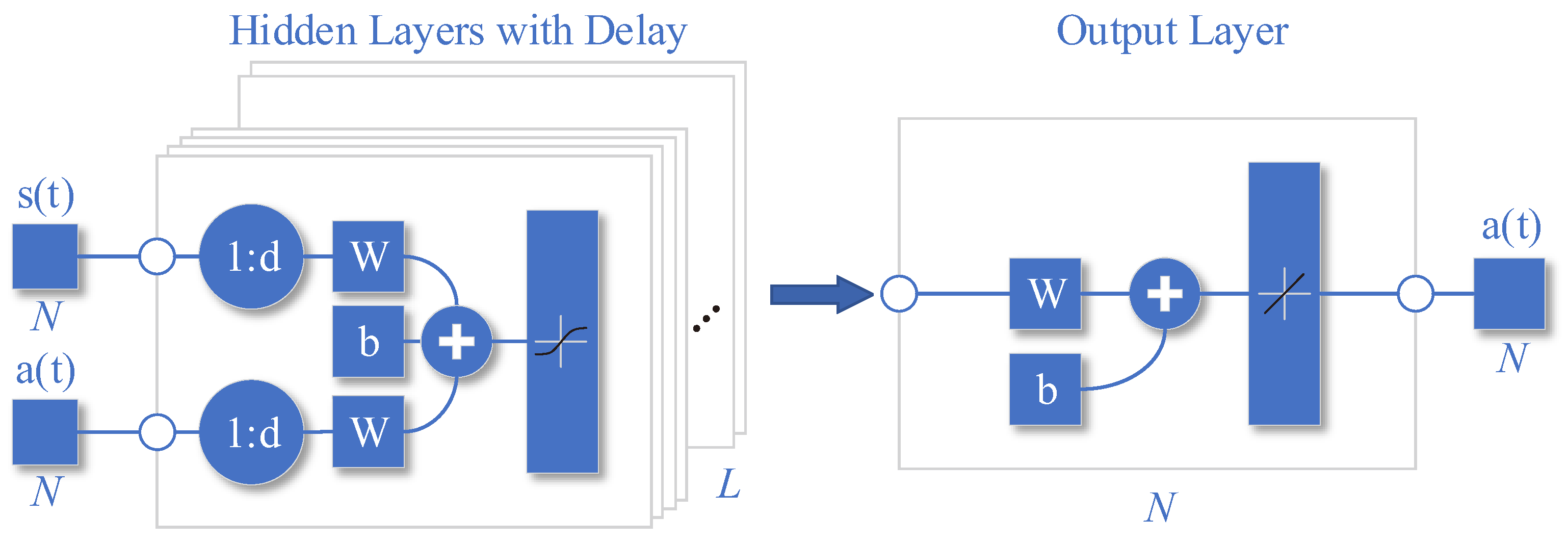
3.3. Imitation Learning Neural Network
As shown in
Figure 3, it is a schematic diagram of the network structure of the trained ILNN. The trained ILNN should predict the next maximum reward action based on the past state and action of the past
timeslots:
Here, the neural network
can be expressed as a mapping from the input state domain
to the output action domain
, that is,
. Considering each hidden layer as a transformation function, the neural network can be expressed as
where
g is the output layer transformation function,
is the
ith hidden layer, and
L is the number of hidden layers, the hidden layer can be expressed as follows:
where
and
to
are the transformation functions of the hidden layer. The transformation function of the hidden layer and the output layer can be broken down into linear transformation and nonlinear transformation. The linear transformation is the product of the weight vector and the input vector plus the bias variable, and the nonlinear transformation is the nonlinear activation. Then
can be expressed as follows:
Here, and are the weight vector and bias variable of the ith layer, respectively.
The specific process of the network structure is expressed in the following:
where
is the hidden layer output matrix,
is the hidden layer historical state weight parameter group,
is the hidden layer historical action weight parameter group, b1 is the hidden layer offset parameter group,
is the output layer weight parameter group, and
is the output layer offset parameter group.
The state input of the network is the concatenation of the state vectors of the past
timeslots, represented as
,
While the action input is the concatenation of the state vectors of the past
timeslots, represented as
,
The activation function used is
,
due to its fully differentiable, antisymmetric, and symmetric center at the origin characteristics, making it a commonly used activation function of the hidden layer.
The network training process is formalized in
where
is the network parameter group, including
,
,
,
,
. The network parameters are adjusted to minimize the gap between the reward of the network strategy and the expert strategy, obtaining the output result
of imitation learning.
3.4. Decision Making
The output
of the ILNN is an
sequential array of decimal numbers. To reduce the influence of error on channel selection and make channels with similar values have similar selection probability,
is used as the selection probability of decision action after exponential compression and normalization, represented by
where
is the selection probability of the anti-jamming action
obtained by channel selection according to
probability.
4. Simulation
This section presents the simulation results of this manuscript from four aspects: jamming settings, simulation settings, performance experiments, and comparative experiments. The jamming settings part introduces a jamming environment where jamming appears in various patterns alternately. The simulation setting introduces the definition of several important concepts in this section. The performance experiments part demonstrates the impact of different numbers of hidden layers in the neural network and sample delays on the anti-jamming performance. The comparative experiments part compares the proposed method in this manuscript with a DQN-based anti-jamming method. However, our source code is unfortunately not available due to the requirements of the organization. We will actively communicate with any researcher who is interested in this paper and send us an email.
4.1. Jamming Setting
In the scenario of this manuscript, the corresponding state samples are as follows. Taking
M timeslots as a sample, each sample is divided into
k parts with long random timeslot lengths and their jamming parameters are randomly generated. Then a jamming sample is given by:
among them, there are
time nodes,
, such that
here,
,
is the SJ,
is the NSJ,
is the CJ,
is the CSJ, and
is the DJ.
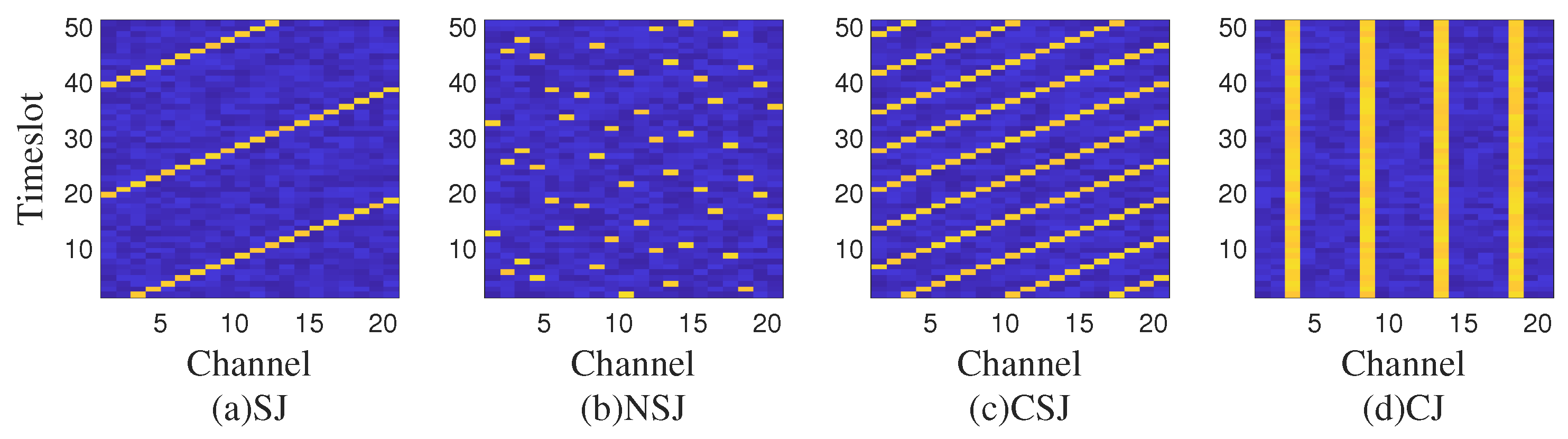
In this manuscript, we consider a scenario where two different malicious jammers are present: the determined jammer and the dynamic jammer. As shown in
Figure 4, they use different jamming techniques, and they jam in the following ways, respectively:
Determined jammer (DJ): The jammer selects a channel for a period of time to continuously jam the channel.
Dynamic jammer: The jammer alternately uses Sweep Jamming (SJ), Nonlinear Sweep Jamming (NSJ), Comb Jamming (CJ), and Comb Sweep Jamming (CSJ).
Among them, for a single channel, the jamming signal is blocking jamming, that is, in the channel where the jamming signal is located, the communication cannot communicate normally. The research focus of the anti-jamming decision problem is to select a channel and transmit power in time and effectively to ensure reliable transmission of wireless communication systems by means of machine learning and neural networks.
Each jamming signal can be represented as follows.
4.1.1. Sweep Jamming
where
is the start channel of the sweep jamming,
is the channel offset of the sweep jamming, that is, the next moment is several channels to the right compared with the previous moment,
is the sweep jamming power.
,
means that on the basis of
, the
th term
is equal to
. In general, in order to traverse all channels,
and
should have no common factors other than 1.
4.1.2. Nonlinear Sweep Jamming
where
is the nonlinear sweep pattern,
is the nonlinear sweep period, and
is the nonlinear sweep jamming power.
4.1.3. Comb Jamming
where
is the comb-jamming starting channel,
is the comb-jamming channel interval, and
is the comb-jamming power.
represents an array starting from
, separated by
, and not exceeding
at most. For example,
,
,
. Then the comb jamming signal
.
4.1.4. Comb Sweep Jamming
where
is the initial frequency of comb sweep jamming,
is the channel shift of comb sweep jamming,
is the channel interval of comb sweep jamming, and
is the power of comb sweep jamming.
4.1.5. Determined Jamming
where
is the jamming channel of fixed-frequency jamming, and
is the fixed-frequency jamming power.
4.2. Simulation Setting
The software and hardware information of the performance experiment is shown in
Table 2. We used MATLAB (2021a) to generate the data, Python (3.8) to perform machine learning, and the data were stored in .mat files. The machine learning library we used was TensorFlow1.14.
The simulation parameters of the performance experiment are shown in
Table 3. Simulation parameters mean that this manuscript considers a multi-channel communication scenario with 20 channels, each with a channel bandwidth of 2 MHz, and takes 1000 timeslot as a communication unit, in which the aforementioned jamming pattern will alternate randomly.
The simulation experiments focus on the collision rate as the main performance metric, specifically examining the performance variations of the proposed approach when the jamming pattern switches, the jamming-to-noise ratio (JNR) changes, and the proportion of jamming signals changes. The key concepts are defined as follows:
Collision rate: The ratio of the number of collisions between the communication signal and the jamming signal in the same timeslot in the same channel to the total number of timeslots.
Jamming-to-noise ratio (JNR): The decibel ratio of the jamming signal strength in a specific time slot and channel to the intensity of the background Gaussian noise signal in that timeslot. Generally, a lower JNR indicates less noticeable jamming, making it more challenging for the ILNN to make decisions and resulting in a higher collision rate.
Proportion of jamming signals: The ratio of the cumulative number of channels occupied by the jamming signal over a certain number of timeslots to the product of the number of timeslots and the number of channels of interest. Generally, a higher proportion of jamming signals indicates fewer available channels and greater difficulty in resisting jamming, resulting in a higher collision rate.
In the performance experiments, the influence of the number of hidden layers and the number of sample delays on network performance is studied. The key concepts are:
Hidden: The number of hidden layers of the ILNN. Generally, a higher number of hidden layers indicates a stronger expressive power of the neural network, smaller fitting errors, but also longer training and execution times.
Delay: The number of past timeslot samples used by the ILNN for decision-making. Generally, a larger number of delays provides more information for the ILNN to make decisions, leading to more informed decisions. However, it also makes it more difficult to converge when the jamming pattern changes, as it is more influenced by the previous pattern.
4.3. Performance Experiment
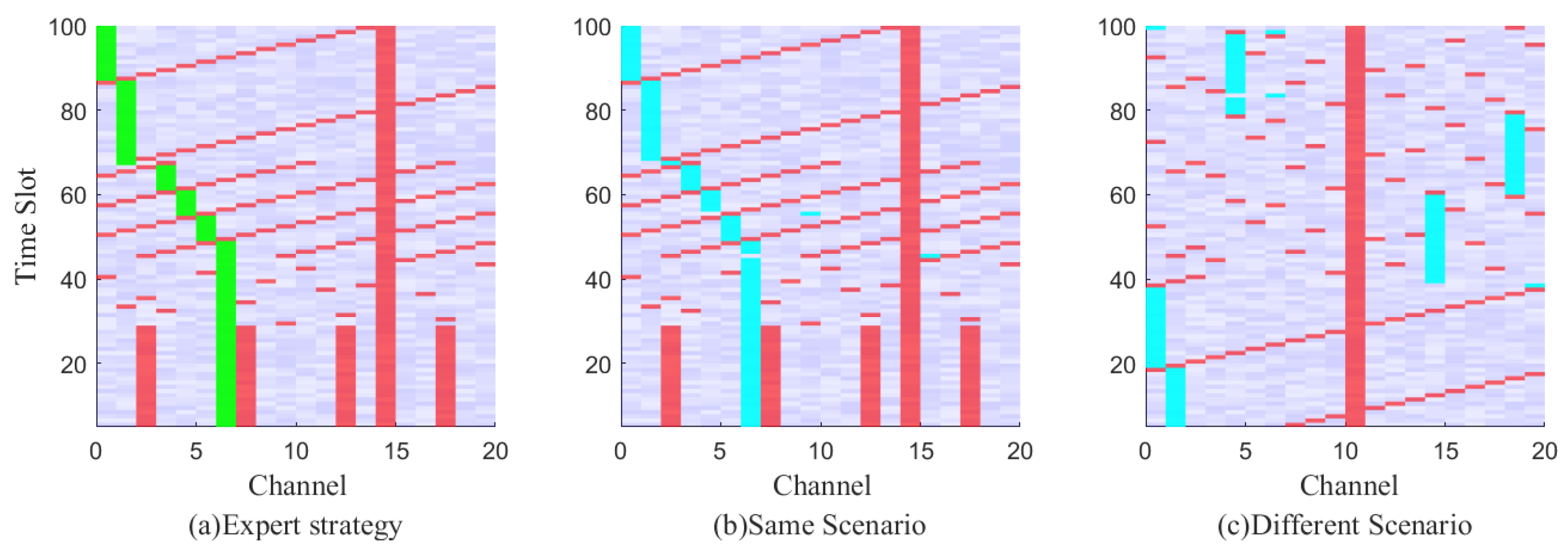
As depicted in
Figure 5, the spectrum anti-jamming process is graphically displayed.
Figure 5a illustrates a schematic diagram of channel selection based on expert strategy. The green block represents the channel selected according to the expert strategy, the red block represents jamming, and the blue-purple block represents the noise background.
Figure 5b shows the channel selection method obtained through real-time decision using the imitation strategy under the same scenario as
Figure 5a, and the blue block represents the channel selected according to real-time decision. In
Figure 5c, the channel selection method obtained through the imitation strategy after a real-time decision is presented in a different scenario from
Figure 4a. The proposed method efficiently solves the decision problem in dynamic jamming scenarios.
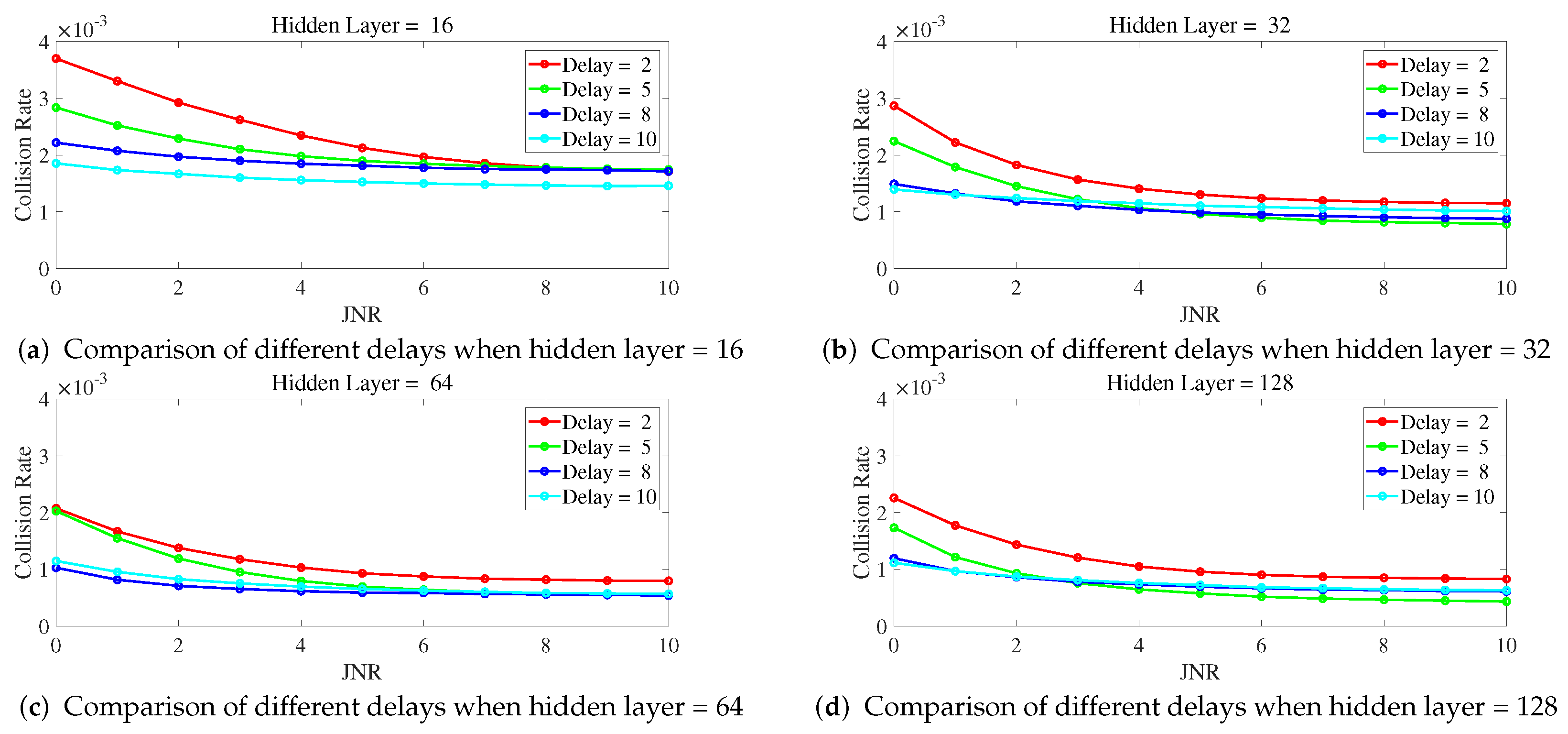
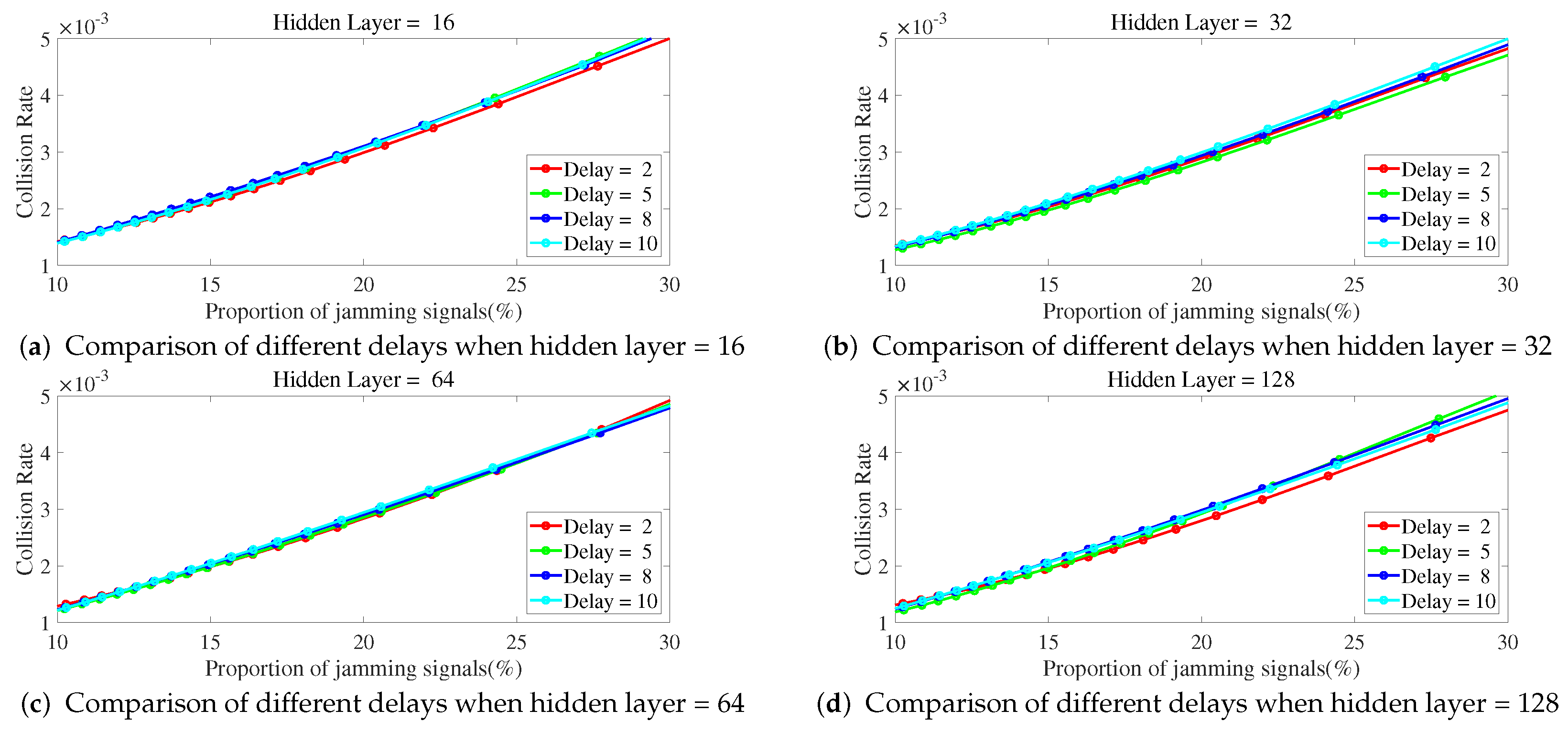
Below is a study on the impact of different parameters of ILNN on anti-jamming performance, with a focus on the number of hidden layers and sample delay in ILNN. Simulations were conducted to observe the collision rate as a function of JNR and the proportion of jamming signals under different ILNN parameters. The network training utilized scaled conjugate gradient which requires less memory and has faster training speed, with a total of 1000 iterations.
Figure 6 illustrates the variation of collision rate as JNR changes for different numbers of hidden layers when a delay is fixed. From
Figure 6, it can be observed that with a fixed delay, a higher number of hidden layers leads to a lower collision rate. In particular, the curve for ILNN with 16 hidden layers shows significantly higher collision rates compared to other curves, indicating inadequate expressive power with 16 hidden layers. On the other hand, the curves for ILNN with 64 and 128 hidden layers exhibit similar trends, and even at a delay of 8, as shown in
Figure 6c, the ILNN with 64 hidden layers demonstrates a lower collision rate. This suggests that the ILNN with 128 hidden layers has excessive expressive power under this condition and, due to limited training iterations, cannot be adequately trained, resulting in similar or even lower anti-jamming performance compared to the ILNN with 64 hidden layers.
Figure 7 shows the variation of collision rate as JNR changes for different delays when the number of hidden layers is fixed. From
Figure 7, it can be observed that with a fixed number of hidden layers, a higher delay leads to a lower collision rate. Specifically, the curves for ILNN with a delay of 2 show noticeably higher collision rates compared to the other curves, indicating that the ILNN with a delay of 2 lacks sufficient historical samples as input for making decisions, leading to inadequate anti-jamming capability. The curves for delay = 8 and delay = 10 are similar, with performance lower than that of delay = 8. This is because the limited training iterations prevent them from being adequately trained.
As shown in
Figure 8 and
Figure 9, the collision rate changes with the proportion of jamming signals. As the proportion of jamming signals increases, the collision rate also increases. As shown in
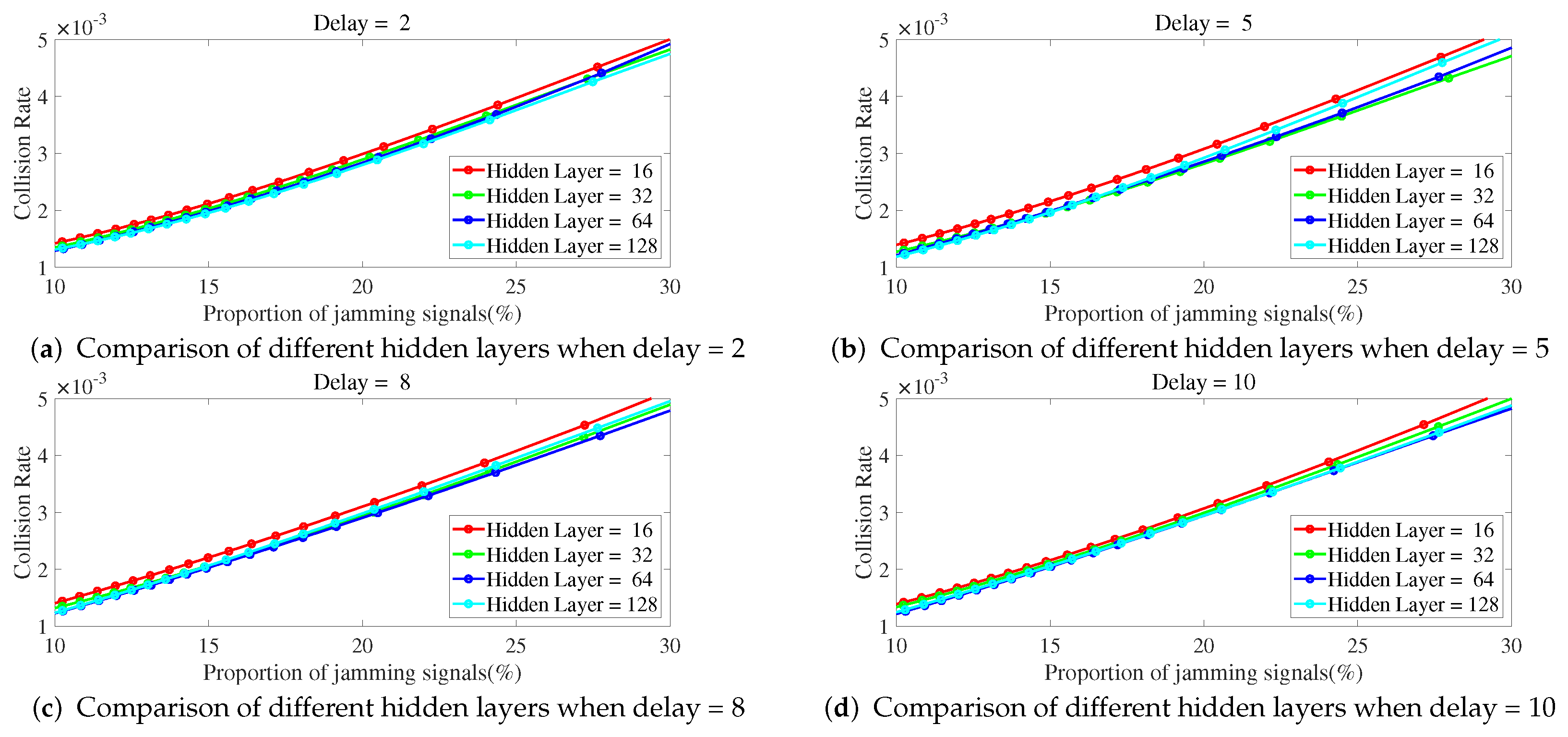
Figure 8, when the delay is fixed, the number of hidden layers is less and the jamming collision rate is higher. The ILNN with 16 hidden layers has the highest jamming collision rate.
As shown in
Figure 9, when the number of hidden layers is fixed, the change of the delay number has little impact on the collision rate when the proportion of jamming signals increases. Therefore, when the proportion of jamming signals increases, it is not feasible to improve the performance of ILNN by only increasing the delay number and participating in more samples of the past time slots without increasing the number of hidden layers of the network.
In summary, increasing the number of hidden layers and delay values can enhance the anti-jamming performance of ILNN when the JNR or proportion of jamming signals increases. However, excessive hidden layers and high delay values do not significantly improve the system’s anti-jamming performance, while also requiring longer training time. Furthermore, higher delay values make the anti-jamming decision more susceptible to the influence of the previous jamming pattern. In the simulation scenario of this manuscript, an ILNN with 128 hidden layers does not show better anti-jamming performance compared to an ILNN with 64 hidden layers. ILNNs with a delay of 8 or 10 do not exhibit better anti-jamming performance compared to an ILNN with a delay of 5. Therefore, in this simulated scenario, an ILNN with 64 hidden layers and a delay of 5 can ensure both anti-jamming performance and a smaller network size. Hence, the comparative experiment in
Section 4.4 selects an ILNN with 64 hidden layers and a delay of 5.
4.4. Comparative Experiments
This subsection presents a comparative analysis between IL-based anti-jamming methods, RL-based anti-jamming methods, and DQN-based anti-jamming methods. It examines the performance curves and the time required for re-stabilization of the three methods when there is a sudden switch in the jamming pattern. Moreover, it investigates the variations in collision rate changes for the three methods as the JNR varies. Additionally, it examines the variations in collision rates for the three methods as the proportion of jamming signals fluctuates.
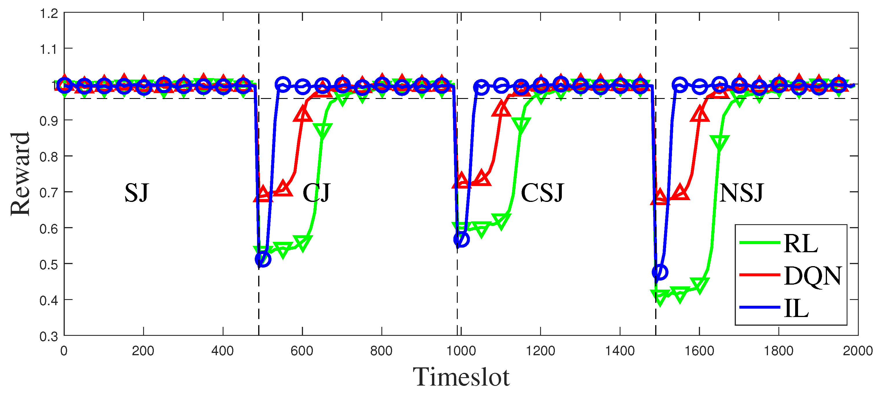
A comparison is made among the proposed methods, RL and DQN.
Figure 10 illustrates the performance transformation curves of IL, converged RL, and converged DQN when faced with sudden switching of jamming patterns. Based on the simulation results, it can be observed that the RL-based and the DQN-based anti-jamming decision methods take a long time to reconverge when the jamming pattern switches, whereas the proposed method can return to a stable state faster despite a sharp performance drop. Apart from the three switching processes depicted in
Figure 10, additional details on the duration of the transitions can be found in
Table 4,
Table 5 and
Table 6. In comparison to RL and DQN, which learn and decide simultaneously as the states change, IL utilizes imitation and generalization from expert strategy that encompass certain jamming-switching processes. Consequently, when the jamming pattern switches, IL demonstrates reduced “decision inertia” toward previous jamming patterns, facilitating more prompt and robust decision-making. Thus, the IL-based approach proposed in this study enables the timely and effective selection of appropriate channels during jamming-type switches, ensuring the reliability and stability of communication systems.
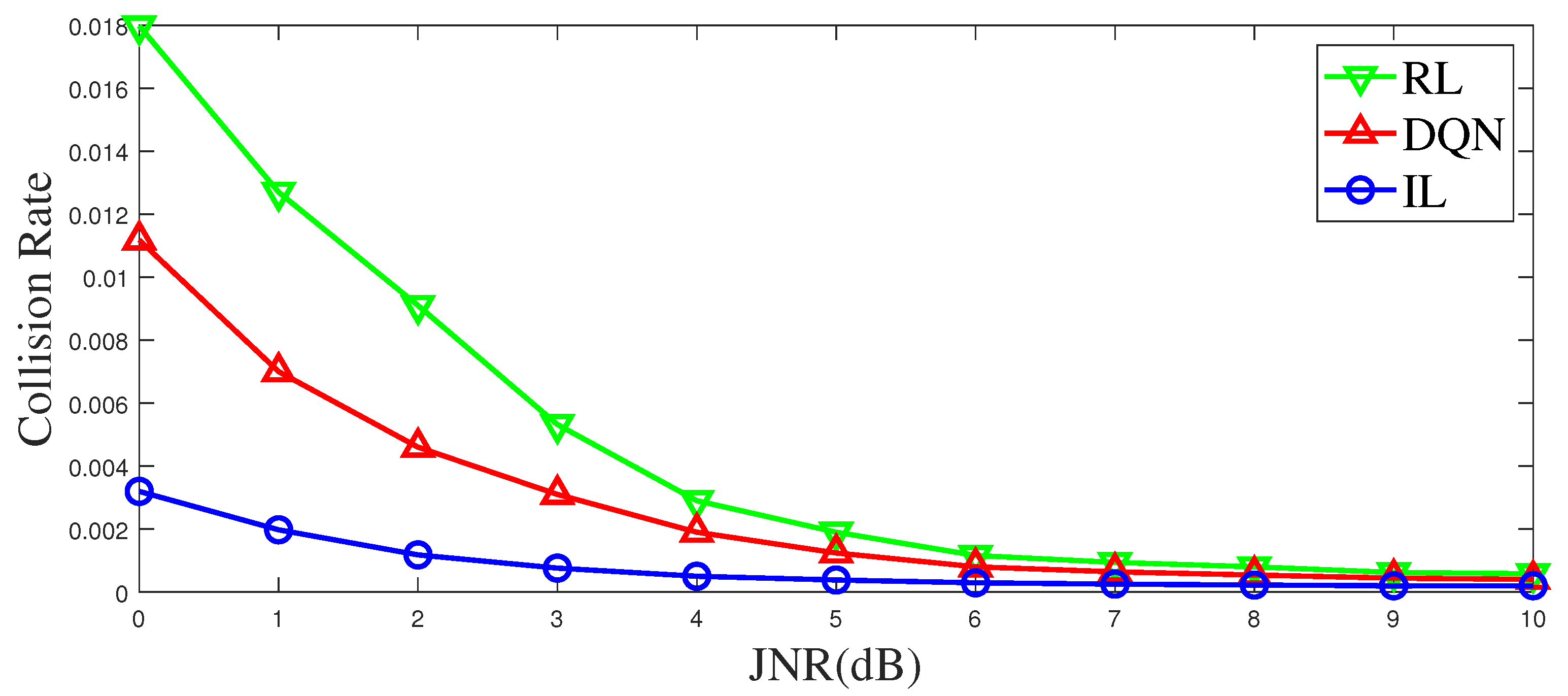
Background noise and channel fading can influence the perception of jamming, which in turn affects the anti-jamming communication. For classical Q-learning, the state space is limited, and the state value is discrete. Generally, a threshold is used to make a decision before learning, but this process causes information loss, affecting learning and decision-making. In this study, the noisy state is directly input to DQN and IL for anti-jamming decisions. For RL, noise affects their sensing of the environment, that is, a large number of misjudgments are generated when it makes a decision on the environment state according to the threshold, which affects the anti-jamming performance of the system. The results are presented in
Figure 11. When considering channel fading and noise, IL has a lower jamming probability than RL and DQN. The IL-based method generalizes the expert strategy from a global perspective, while the RL-based method and the DQN-based methods focus on the change of the current state. So, noise and fading in the IL-based method have an impact on the decision with more overall statistical characteristics, while in the RL-based method and the DQN-based method, noise and fading have an impact on the decision with more individual random characteristics. Therefore, the IL-based method is less affected by noise and fading.
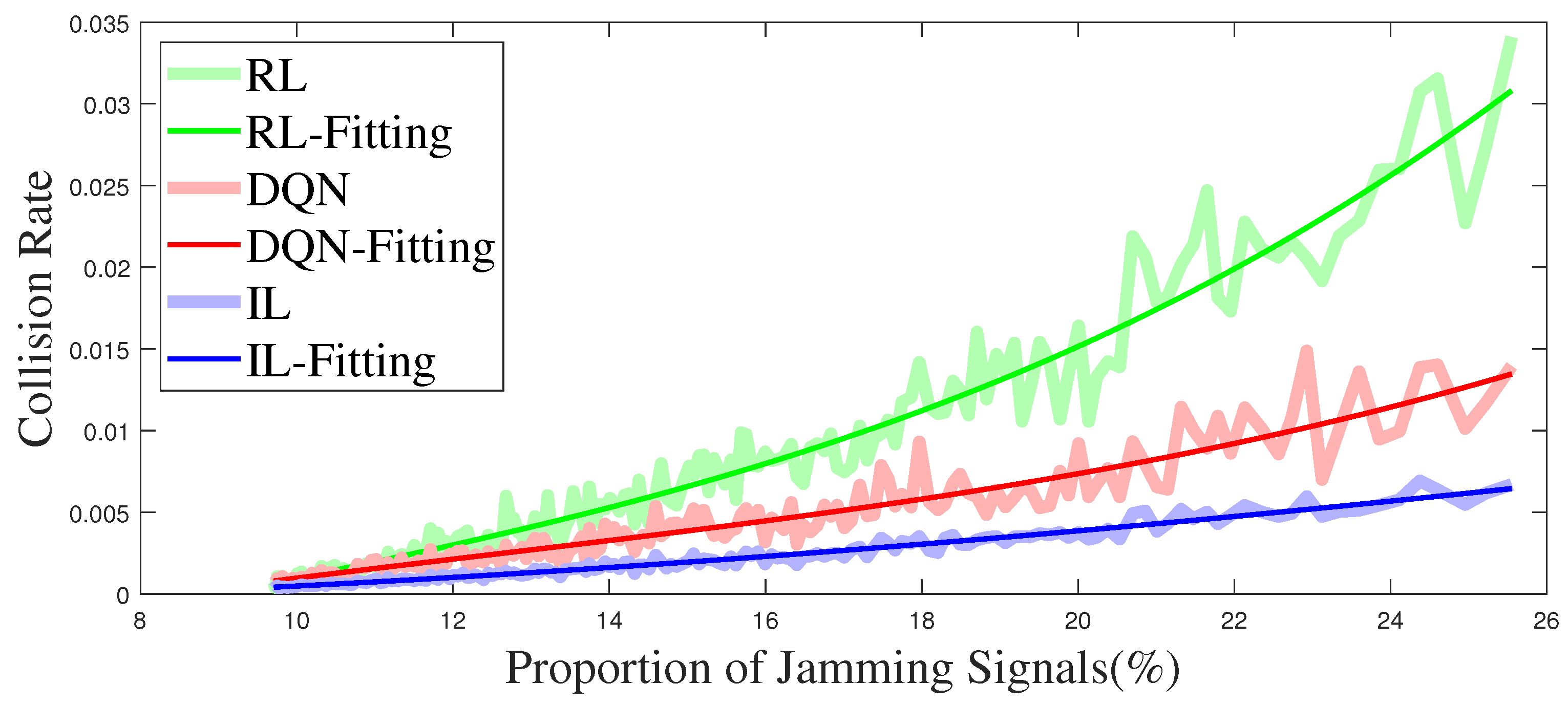
Figure 12 illustrates the relationship between the collision rate and the proportion of jamming signals. The light thick line in the figure is the direct result of the simulation, and the thin line is the curve obtained by fitting. It can be seen from
Figure 12 that the collision rate of the IL anti-jamming method is about 30% lower than that of the DQN-based method and 80% lower than that of the RL-based method under the same proportion of jamming signals. The increase in the proportion of jamming signals means that more channels are jammed, and the RL-based and the DQN-based methods have fewer decision choices in the learning process, making the decision more difficult. However, the training method based on IL has different parameters and expert strategy under different jamming patterns, the influence of an increasing proportion of jamming signals is minimal.
The aforementioned experiments demonstrate that the IL-based anti-jamming method exhibits faster re-stabilization during sudden changes in jamming patterns when compared to the RL-based method and the DQN-based anti-jamming method. Moreover, the IL-based approach shows reduced susceptibility to background noise and channel fading, enabling prompt and effective multi-channel decisions in response to variations in the environment. Additionally, when faced with increasing proportions of jamming signals, the IL-based method proves more efficient in avoiding collisions compared to RL and DQN.
5. Conclusions
The proposed anti-jamming method based on imitation learning generates expert trajectories from historical samples, which are then imitated using ILNN. Users can obtain anti-jamming strategies from the trained ILNN for anti-jamming decision-making. This method enables timely and effective multi-channel decisions in response to changes in the jamming environment. Compared to the DQN-based anti-jamming method, this method exhibits faster convergence when faced with sudden switches in jamming patterns. It is less affected by background noise and channel fading, resulting in a lower collision rate when the proportion of jamming signals increases.
However, this method has limited generalization capability and limited ability to handle jamming patterns beyond those contained in the training samples. Further research and improvement can be conducted by incorporating deep reinforcement learning. The combination of imitation learning, which learns from historical information, and deep reinforcement learning, which adapts to real-time changes in the current environment, can be explored. Additionally, as the number of hidden layers in ILNN increases, its expressive power is enhanced but requires more training time. Moreover, there is a threat of adversarial samples to ILNN. Adversaries can significantly impact the anti-jamming decision-making of ILNN at minimal cost. Targeted optimization can be applied to ILNN by leveraging adversarial training techniques in adversarial machine learning.
In future work, we will consider combining imitation learning with deep reinforcement learning to make more robust intelligent anti-jamming communication decisions, aiming at the problem of poor adaptability when facing new scenarios. Aiming at the problem that imitation learning requires a high number of historical samples, it was considered to combine it with the generative adversarial network, so that the system could train an excellent enough ILNN with limited historical samples.
The advantage of imitation learning lies in obtaining a posteriori optimal trajectory through the analysis of historical samples, and obtaining a better experience for anti-jamming by imitating the posteriori optimal trajectory. Its disadvantage lies in requiring more historical samples for the analysis of posteriori optimal trajectory. Deep reinforcement learning, on the other hand, focuses on solving the problem of the moment, can quickly learn from a new environment, and can perform as it learns. Our initial idea is to trust the results of deep reinforcement learning more when there are fewer historical samples or historical experience has a low anti-jamming reference value to the current scene, and trust the results of imitation learning more when there are enough state experience samples collected for imitation learning. Through such a combination, the system can obtain both the flexibility of deep reinforcement learning and the high accuracy of imitation learning. In the process of combining IL and DQN, we need to increase the storage space complexity and the computational complexity of each timeslot, but we can obtain an anti-jamming communication method with higher accuracy and fewer timeslots. The combined system will converge faster and the convergence value will be higher.
Author Contributions
Conceptualization, Z.Z., Y.N. and W.Z.; Methodology, Z.Z., Y.N. and W.Z.; Software, Z.Z. and B.W.; Validation, Z.Z., Y.N. and B.W.; Formal analysis, Z.Z., B.W. and W.Z.; Resources, Z.Z. and Y.N.; Data curation, B.W.; Writing—original draft, Z.Z.; Writing—review and editing, Z.Z., Y.N. and W.Z.; Supervision, Y.N. All authors have read and agreed to the published version of the manuscript.
Funding
This research was funded by The National Natural Science Foundation of China grant number U19B2014.
Data Availability Statement
The data presented in this study are not available due to privacy.
Conflicts of Interest
The authors declare no conflict of interest.
References
- Chen, L.; Li, Y.; Huang, C.; Li, B.; Xing, Y.; Tian, D.; Li, L.; Hu, Z.; Na, X.; Li, Z.; et al. Milestones in Autonomous Driving and Intelligent Vehicles: Survey of Surveys. IEEE Trans. Intell. Veh. 2023, 8, 1046–1056. [Google Scholar] [CrossRef]
- Gao, Y.; Tong, W.; Wu, E.Q.; Chen, W.; Zhu, G.; Wang, F. Chat with ChatGPT on Interactive Engines for Intelligent Driving. IEEE Trans. Intell. Veh. 2023, 8, 1–3. [Google Scholar] [CrossRef]
- Nar, D.; Kotecha, R. Optimal waypoint assignment for designing drone light show formations. Results Control Optim. 2022, 9, 100174. [Google Scholar] [CrossRef]
- Ye, Z.; Wei, Y.; Li, J.; Yan, G.; Wang, L. A distributed pavement monitoring system based on Internet of Things. J. Traffic Transp. Eng. (Engl. Ed.) 2022, 9, 305–317. [Google Scholar] [CrossRef]
- Zhou, Q.; Niu, Y.; Xiang, P.; Li, Y. Intra-Domain Knowledge Reuse Assisted Reinforcement Learning for Fast Anti-Jamming Communication. IEEE Trans. Inf. Forensics Secur. 2023, 18, 4707–4720. [Google Scholar] [CrossRef]
- Ruby, R.; Yang, H.; Wu, K. Anti-Jamming Strategy for Federated Learning in Internet of Medical Things: A Game Approach. IEEE J. Biomed. Health Inform. 2023, 27, 888–899. [Google Scholar] [CrossRef]
- Nguyen, T.; Nguyen, K. Pilot-partitioning Protocol and Anti-jamming Methods in Distributed Massive MIMO systems. IEEE Trans. Cogn. Commun. Netw. 2023, 9, 1211–1225. [Google Scholar] [CrossRef]
- Im, H.; Lee, S. Anti-Jamming Games in Multi-Band Wireless Ad Hoc Networks. IEEE Trans. Inf. Forensics Secur. 2023, 18, 872–887. [Google Scholar] [CrossRef]
- Liu, X.; Xu, Y.; Jia, L.; Wu, Q.; Anpalagan, A. Anti-jamming communications using spectrum waterfall: A deep reinforcement learning approach. IEEE Commun. Lett. 2018, 22, 998–1001. [Google Scholar] [CrossRef]
- Polak, L.; Milos, J. LTE and LoRa in the 2.4 GHz Band: Adjacent Channel Interference Issues. In Proceedings of the 30th International Conference Radioelektronika (RADIOELEKTRONIKA), Bratislava, Slovakia, 15–16 April 2020. [Google Scholar]
- Polak, L.; Milos, J. Performance analysis of LoRa in the 2.4 GHz ISM band: Coexistence issues with Wi-Fi. Telecommun. Syst. 2020, 74, 299–309. [Google Scholar] [CrossRef]
- Sharma, H.; Kumar, N.; Tekchandani, R. Mitigating Jamming Attack in 5G Heterogeneous Networks: A Federated Deep Reinforcement Learning Approach. IEEE Trans. Veh. Technol. 2023, 72, 2439–2452. [Google Scholar] [CrossRef]
- Wang, T.; Li, Y.; Wu, Y.; Tony, Q. Secrecy driven Federated Learning via Cooperative Jamming: An Approach of Latency Minimization. IEEE Trans. Emerg. Top. Comput. 2022, 10, 1687–1703. [Google Scholar] [CrossRef]
- Nishat, I.; Nguyen, H.; Inshil, D.; Kijoon, C. AFRL: Adaptive federated reinforcement learning for intelligent jamming defense in FANET. J. Commun. Netw. 2020, 22, 244–258. [Google Scholar]
- Yuan, Y.; Zheng, G.; Wong, K.; Ottersten, B.; Luo, Z. Transfer Learning and Meta Learning-Based Fast Downlink Beamforming Adaptation. IEEE Trans. Wirel. Commun. 2021, 20, 1742–1755. [Google Scholar] [CrossRef]
- Zhu, X.; Li, S. MGML: Momentum Group Meta-Learning for Few-Shot Image Classification. Neurocomputing 2022, 514, 351–361. [Google Scholar] [CrossRef]
- Liu, M.; Liu, Z.; Lu, W.; Chen, Y.; Gao, X.; Zhao, N. Distributed Few-Shot Learning for Intelligent Recognition of Communication Jamming. IEEE J. Sel. Top. Signal Process. 2022, 16, 395–405. [Google Scholar] [CrossRef]
- Zhou, Q.; Li, Y.; Niu, Y. Intelligent anti-jamming communication for wireless sensor networks: A multi-agent reinforcement learning approach. IEEE Open J. Commun. Soc. 2021, 2, 775–784. [Google Scholar] [CrossRef]
- Yin, Z.; Lin, Y.; Zhang, Y.; Qian, Y.; Shu, F.; Li, J. Collaborative multiagent reinforcement learning aided resource allocation for uav anti-jamming communication. IEEE Internet Things J. 2022, 9, 23995–24008. [Google Scholar] [CrossRef]
- Pourranjbar, A.; Kaddoum, G.; Aghababaiyan, K. Deceiving-based anti-jamming against single-tone and multitone reactive jammers. IEEE Trans. Commun. 2022, 70, 6133–6148. [Google Scholar] [CrossRef]
- Liu, X.; Xu, Y.; Cheng, Y.; Li, Y.; Zhao, L.; Zhang, X. A heterogeneous information fusion deep reinforcement learning for intelligent frequency selection of hf communication. China Commun. 2018, 15, 73–84. [Google Scholar] [CrossRef]
- Yao, Y.; Zhao, J.; Li, Z.; Cheng, X.; Wu, L. Jamming and eavesdropping defense scheme based on deep reinforcement learning in autonomous vehicle networks. IEEE Trans. Inf. Forensics Secur. 2023, 18, 1211–1224. [Google Scholar] [CrossRef]
- Li, H.; Zhang, S.; Fang, Z.; Qiu, Q. Ucb-dqn based joint beamforming and power control for software defined uav swarm network. J. Phys. Conf. Ser. 2023, 2224, 012101. [Google Scholar] [CrossRef]
- Niu, Y.; Zhou, Z.; Pu, Z.; Wan, B. Anti-Jamming Communication Using Slotted Cross Q Learning. Electronics 2023, 12, 2879. [Google Scholar] [CrossRef]
- Ding, H.; Zhou, Q.; Niu, Y.; Xiang, P.; Zhou, Z. A discounted-UCB1-tuned plus Q-learning based anti-jamming routing algorithm for wireless mesh networks. Electron. Lett. 2023, 59, 12895. [Google Scholar] [CrossRef]
- Zeng, P.; Liu, A.; Zhu, C.; Wang, T.; Zhang, S. Trust-based multi-agent imitation learning for green edge computing in smart cities. IEEE Trans. Green Commun. Networkingy 2022, 6, 1635–1648. [Google Scholar] [CrossRef]
- Xiao, Y.; Sun, Z.; Shi, G.; Niyato, D. Imitation learning-based implicit semantic-aware communication networks: Multi-layer representation and collaborative reasoning. IEEE J. Sel. Areas Commun. 2023, 41, 639–658. [Google Scholar] [CrossRef]
- Huang, S.; Zhang, Z.; Wang, S.; Wang, R.; Huang, K. Accelerating federated edge learning via topology optimization. IEEE Internet Things J. 2023, 10, 2056–2070. [Google Scholar] [CrossRef]
Figure 2.
Method process structure.
Figure 2.
Method process structure.
Figure 3.
Imitation Learning Neural Network.
Figure 3.
Imitation Learning Neural Network.
Figure 4.
Time-frequency waterfall figure of the spectrum anti-jamming process.
Figure 4.
Time-frequency waterfall figure of the spectrum anti-jamming process.
Figure 5.
Time-frequency waterfall figure of the spectrum anti-jamming process. The red block represents the jamming signal, the lavender is the background noise, the green block is the communication trajectory selected according to the expert strategy, and the blue block is the user communication trajectory selected after imitation learning.
Figure 6.
The delay is fixed, and the collision rate cha nges curve with JNR under different hidden layers.
Figure 6.
The delay is fixed, and the collision rate cha nges curve with JNR under different hidden layers.
Figure 7.
The hidden layers is fixed, and the collision rate changes curve with JNR under different delay.
Figure 7.
The hidden layers is fixed, and the collision rate changes curve with JNR under different delay.
Figure 8.
The delay is fixed, and the collision rate changes curve with the proportion of jamming signals under different hidden layers.
Figure 8.
The delay is fixed, and the collision rate changes curve with the proportion of jamming signals under different hidden layers.
Figure 9.
The hidden layers are fixed, and the collision rate changes curve with the proportion of jamming signals under different delays.
Figure 9.
The hidden layers are fixed, and the collision rate changes curve with the proportion of jamming signals under different delays.
Figure 10.
Comparison of anti-jamming performance among RL, DQN and IL when jamming pattern is switched.
Figure 10.
Comparison of anti-jamming performance among RL, DQN and IL when jamming pattern is switched.
Figure 11.
The collision rate varies with the JNR of jamming signals.
Figure 11.
The collision rate varies with the JNR of jamming signals.
Figure 12.
The collision rate varies with the proportion of jamming signals.
Figure 12.
The collision rate varies with the proportion of jamming signals.
Table 1.
Summary of Related Research.
Table 1.
Summary of Related Research.
| Reference | Year | Research Area | Technical Scheme | Method | Weakness |
|---|
| [10] | 2020 | LTE & LoRa | Automated Laboratory
Measurement | Automatic Control
Method | Historical experience
is underutilized |
| [11] | 2020 | IoT | Automated Measurement |
| [12] | 2023 | 5G | FDRL | FL | Performance is
sacrificed for security |
| [13] | 2022 | Secrecy-driven FL | FL |
| [14] | 2022 | FANET | AFRL |
| [15] | 2021 | Beamforming | Meta Learning | Meta-L | High computing
power requirements |
| [16] | 2022 | Image Classification | MGML |
| [17] | 2020 | Jamming Recognition | Meta Learning |
| [18] | 2021 | Wireless sensor networks | JMAA | RL | Curse of dimensionality;
Unable to cope with
continuous-state Spaces |
| [19] | 2022 | UAV Anti-Jamming
Communication | CMRL |
| [20] | 2022 | Deceiving-based
anti-jamming methods | Reinforcement Learning |
| [21] | 2018 | Frequency Selection
of HF Communication | Deep Reinforcement Learning | DRL | Low sampling efficiency;
Unsteadiness |
| [22] | 2023 | Autonomous
Vehicle Networks | Deep Reinforcement Learning |
| [23] | 2022 | UAV Swarm Network | UCB-DQN |
Table 2.
Hardware and Software.
Table 2.
Hardware and Software.
| Parameters
| Value |
|---|
| CPU | i7-12700K |
| GPU | RTX-3060Ti |
| Data Generation Environment | MATLAB (2021a) |
| Machine Learning Environment | Python (3.8) |
| Data Storage Format | .mat |
| Algorithms Library | TensorFlow 1.14 |
Table 3.
Simulation Parameters.
Table 3.
Simulation Parameters.
| Parameters | Value |
|---|
| Layers | 16, 32, 64, 128 |
| Delay | 2, 5, 8, 10 |
| Length of Timeslot | 1 ms |
| Channel Bandwidth | 2 MHz |
| Number of Channels | 20 |
| Number of Timeslots for one communication unit | 1000 |
Table 4.
Duration of restabilization after jamming pattern switch of RL.
Table 4.
Duration of restabilization after jamming pattern switch of RL.
| | After | CJ | SJ | CSJ | NSJ |
|---|
| Before | |
|---|
| CJ | 0 | 225.49 | 219.41 | 246.92 |
| SJ | 239.46 | 0 | 233.14 | 243.27 |
| CSJ | 256.71 | 202.22 | 0 | 250.06 |
| NSJ | 251.79 | 206.98 | 230.69 | 0 |
Table 5.
Duration of restabilization after jamming pattern switch of DQN.
Table 5.
Duration of restabilization after jamming pattern switch of DQN.
| | After | CJ | SJ | CSJ | NSJ |
|---|
| Before | |
|---|
| CJ | 0 | 120.06 | 115.81 | 145.27 |
| SJ | 125.85 | 0 | 124.08 | 152.43 |
| CSJ | 143.91 | 96.34 | 0 | 142.46 |
| NSJ | 138.91 | 91.97 | 135.01 | 0 |
Table 6.
Duration of restabilization after jamming pattern switch of IL.
Table 6.
Duration of restabilization after jamming pattern switch of IL.
| | After | CJ | SJ | CSJ | NSJ |
|---|
| Before | |
|---|
| CJ | 0 | 63.75 | 58.25 | 39.58 |
| SJ | 47.97 | 0 | 57.96 | 46.51 |
| CSJ | 45.63 | 31.15 | 0 | 45.99 |
| NSJ | 57.71 | 34.19 | 62.40 | 0 |
| Disclaimer/Publisher’s Note: The statements, opinions and data contained in all publications are solely those of the individual author(s) and contributor(s) and not of MDPI and/or the editor(s). MDPI and/or the editor(s) disclaim responsibility for any injury to people or property resulting from any ideas, methods, instructions or products referred to in the content. |
© 2023 by the authors. Licensee MDPI, Basel, Switzerland. This article is an open access article distributed under the terms and conditions of the Creative Commons Attribution (CC BY) license (https://creativecommons.org/licenses/by/4.0/).


