
Denoising Non-Stationary Signals via Dynamic Multivariate Complex Wavelet Thresholding


Abstract
1. Introduction
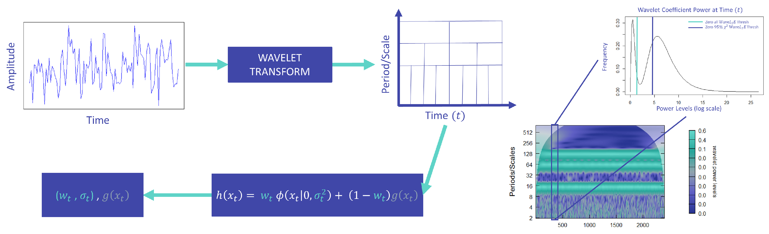
2. Methods
2.1. Wavelets
2.1.1. CWT
2.2. Threshold
2.3. Dynamic Threshold
- Calculate the wavelet transform of the observed time series and recover the squared wavelet coefficients.
- Apply the and at each time point, solving for the estimates of the criterion.
- Threshold the wavelet coefficients based on the estimates.
- Calculate the inverse transform of the denoised time series or solve for the pure signal using the recovered estimates.
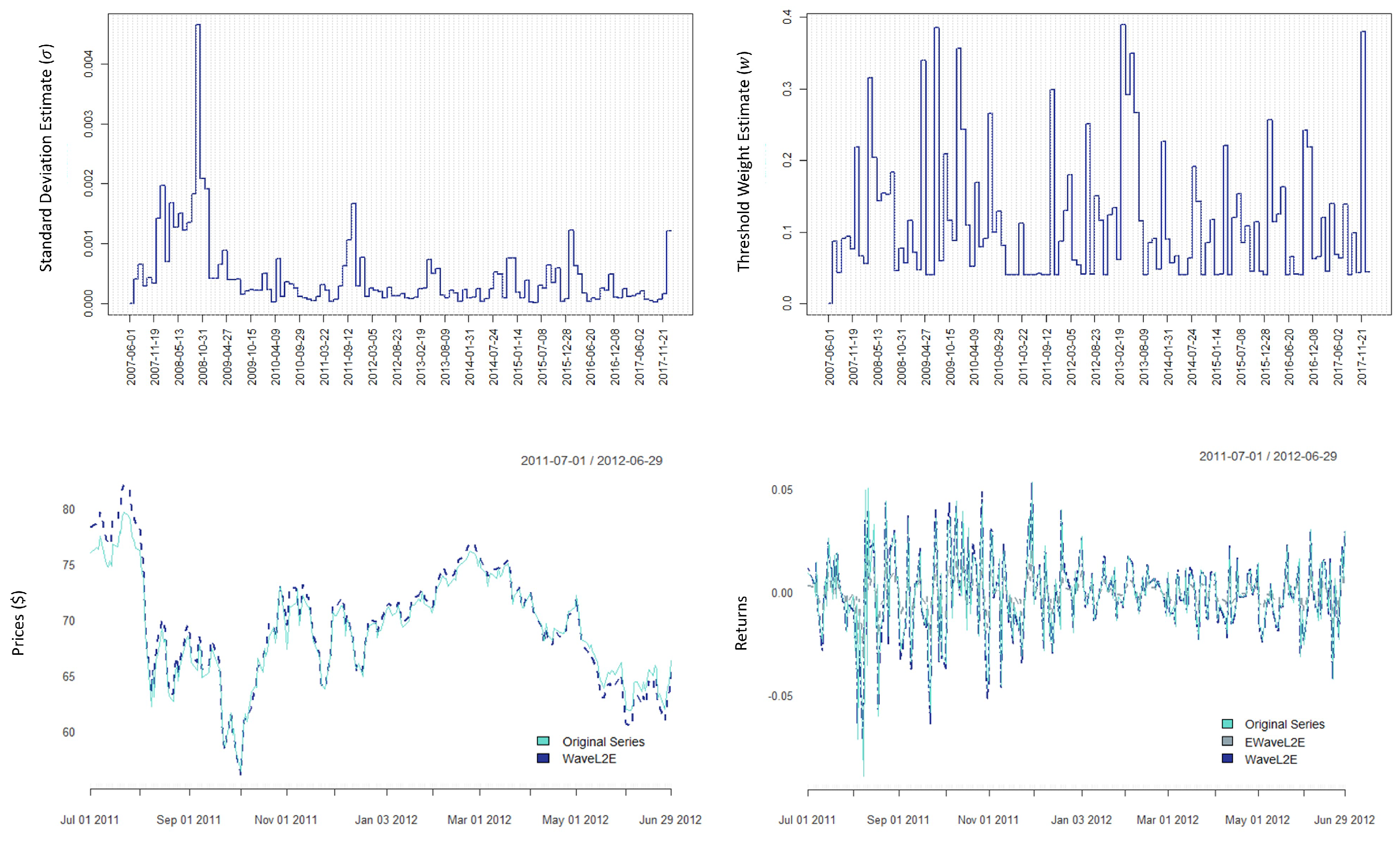
3. Results and Comparative Analysis
3.1. Inter-Scale and Intra-Scale
3.2. Comparative Analysis
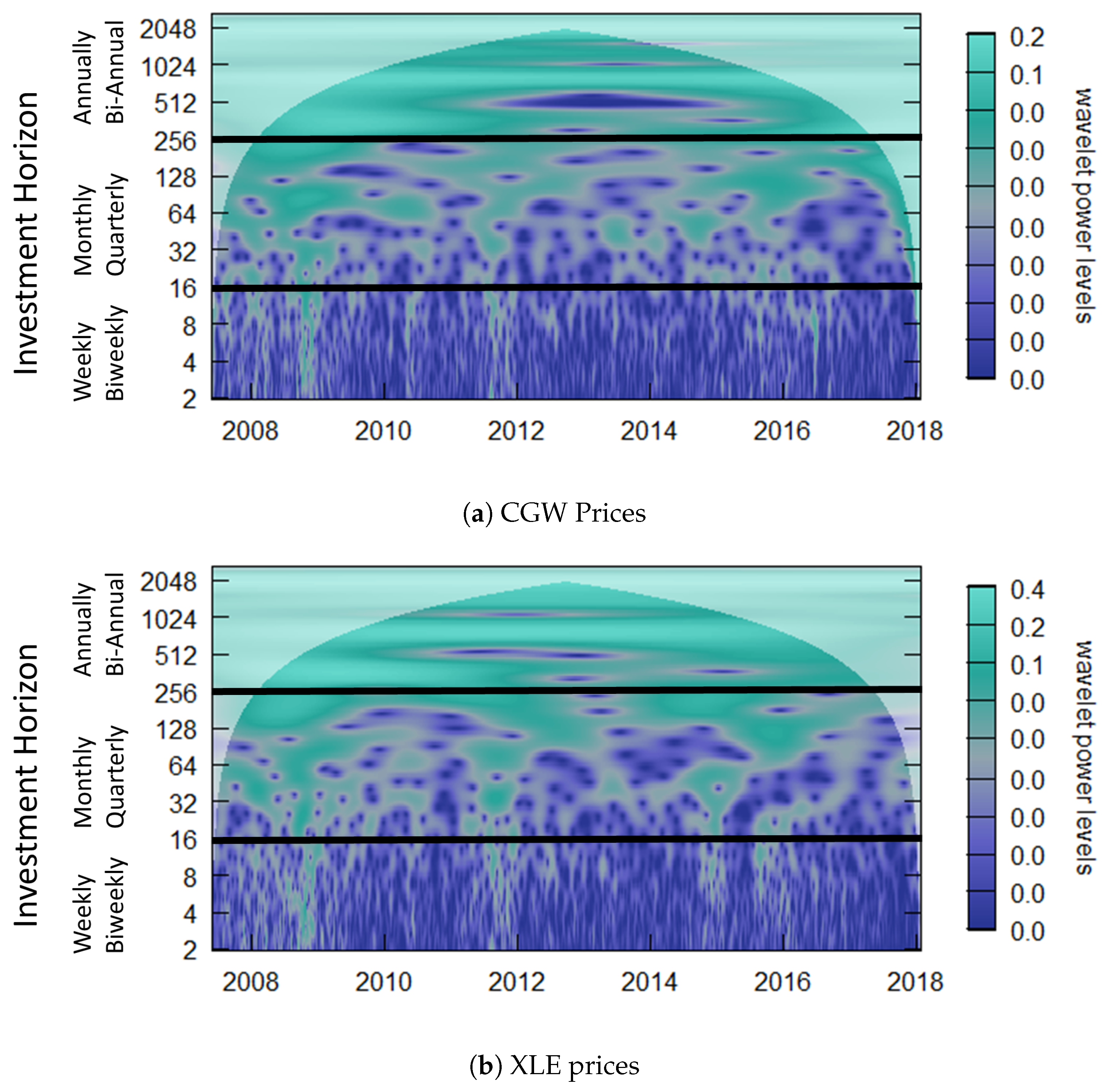
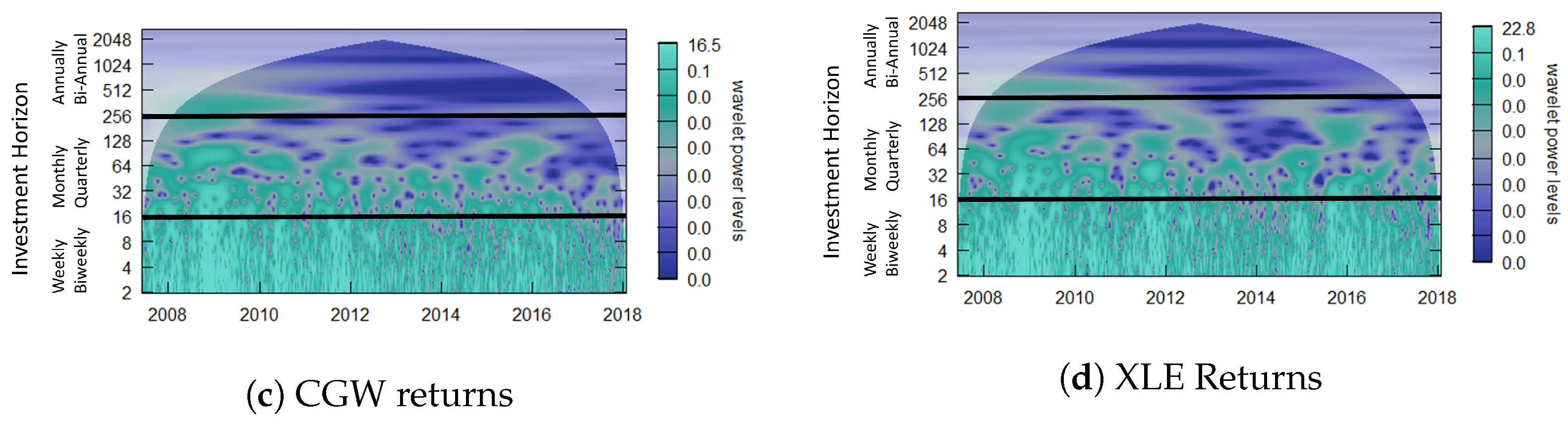
4. Motivating Example: Water–Energy Nexus
5. Conclusions
Author Contributions
Funding
Data Availability Statement
Conflicts of Interest
Abbreviations
| CGW | Global Water Fund |
| CWT | Continuous Wavelet Transform |
| ETF | Exchange Traded Fund |
| GS | Gold Standard |
| ISE | Integrated Squared Error |
| Integrated Squared Error Estimation Criterion | |
| PSA | Percentage of Significant Area |
| PTV | Percentage of Total Volume |
| RMSE | Root-Mean-Squared Error |
| SNR | Signal-to-Noise Ratio |
| WSC | Wavelet-Squared Coherence |
| XLE | Energy Select Sector |
Appendix A
References
- Rostan, P.; Rostan, A. The versatility of spectrum analysis for forecasting financial time series. J. Forecast. 2018, 37, 327–339. [Google Scholar] [CrossRef]
- Wang, G.J.; Xie, C.; Chen, S. Multiscale correlation networks analysis of the US stock market: A wavelet analysis. J. Econ. Interact. Coord. 2017, 12, 561–594. [Google Scholar] [CrossRef]
- Ftiti, Z.; Jawadi, F.; Louhichi, W. Modelling the relationship between future energy intraday volatility and trading volume with wavelet. Appl. Econ. 2017, 49, 1981–1993. [Google Scholar] [CrossRef]
- Kumar, S.; Pathak, R.; Tiwari, A.K.; Yoon, S.M. Are exchange rates interdependent? Evidence using wavelet analysis. Appl. Econ. 2017, 49, 3231–3245. [Google Scholar] [CrossRef]
- Chaudhuri, S.; Lo, A. Spectral Portfolio Theory; Technical report; MIT Sloan School of Management: Cambridge, MA, USA, 2016. [Google Scholar] [CrossRef]
- Nicolis, O.; Mateu, J.; Contreras-Reyes, J.E. Wavelet-Based Entropy Measures to Characterize Two-Dimensional Fractional Brownian Fields. Entropy 2020, 22, 196. [Google Scholar] [CrossRef]
- In, F.; Kim, S. An Introduction to Wavelet Theory in Finance: A Wavelet Multiscale Approach; World Scientific: Singapore, 2012; p. 204. [Google Scholar]
- Reményi, N.; Vidakovic, B. Bayesian nonparametric regression using complex wavelets. arXiv 2018, arXiv:1803.02532. [Google Scholar]
- Barber, S.; Nason, G.P. Real nonparametric regression using complex wavelets. J. R. Statist. Soc. B 2004, 66, 927–939. [Google Scholar] [CrossRef]
- Johnstone, I.M.; Silverman, B.W. Empirical Bayes selection of wavelet thresholds. Ann. Stat. 2005, 33, 1700–1752. [Google Scholar] [CrossRef]
- Donoho, D.L.; Johnstone, I.M. Adapting to Unknown Smoothness via Wavelet Shrinkage. J. Am. Stat. Assoc. 1995, 90, 1200–1224. [Google Scholar] [CrossRef]
- Xiao, F.; Zhang, Y. A Comparative Study on Thresholding Methods in Wavelet-based Image Denoising. Procedia Eng. 2011, 15, 3998–4003. [Google Scholar] [CrossRef]
- Cai, T.T.; Zhou, H.H. A data-driven block thresholding approach to wavelet estimation. Ann. Stat. 2009, 37, 569–595. [Google Scholar] [CrossRef]
- He, C.; Xing, J.; Li, J.; Yang, Q.; Wang, R. A New Wavelet Threshold Determination Method Considering Interscale Correlation in Signal Denoising. Math. Probl. Eng. 2015, 2015, 280251. [Google Scholar] [CrossRef]
- Aguiar-Conraria, L.; Soares, M.J.; Aguiar-Conraria, L. The Continuous Wavelet Transform: Moving beyond uni- and bivariate analysis. J. Econ. Surv. 2014, 28, 344–375. [Google Scholar] [CrossRef]
- Scott, D.W. Parametric statistical modeling by minimum integrated square error. Technometrics 2001, 43, 274–285. [Google Scholar] [CrossRef]
- Scott, A. Denoising by Wavelet Thresholding Using Multivariate Minimum Distance Partial Density Estimation. Ph.D. Thesis, Rice University, Houston, TX, USA, 2006. [Google Scholar]
- Raath, K. Dynamic Multivariate Wavelet Signal Extraction and Forecasting with Applications to Finance. Ph.D. Thesis, Rice University, Houston, TX, USA, 2020. [Google Scholar]
- Raath, K.C.; Ensor, K.B. Time-varying wavelet-based applications for evaluating the Water-Energy Nexus. Front. Energy Res. 2020, 8, 118. [Google Scholar] [CrossRef]
- Raath, K.C.; Ensor, K.B. Wavelet-L2E Stochastic Volatility Models: An Application to the Water-Energy Nexus. Sankhya B 2020, 85, 150–176. [Google Scholar] [CrossRef]
- Torrence, C.; Compo, G.P.; Torrence, C.; Compo, G.P. A Practical Guide to Wavelet Analysis. Bull. Am. Meteorol. Soc. 1998, 79, 61–78. [Google Scholar] [CrossRef]
- Aguiar-Conraria, L.; Azevedo, N.; Soares, M.J. Using wavelets to decompose the time–frequency effects of monetary policy. Physica A 2008, 387, 2863–2878. [Google Scholar] [CrossRef]
- Reboredo, J.C.; Rivera-Castro, M.A.; Ugolini, A. Wavelet-based test of co-movement and causality between oil and renewable energy stock prices. Energy Econ. 2017, 61, 241–252. [Google Scholar] [CrossRef]
- Lilly, J.; Olhede, S. Higher-Order Properties of Analytic Wavelets. IEEE Trans. Signal Process. 2009, 57, 146–160. [Google Scholar] [CrossRef]
- Addison, P.S. The Illustrated Wavelet Transform Handbook: Introductory Theory and Applications in Science, Engineering, Medicine and Finance, 2nd ed.; CRC Press: Boca Raton, FL, USA, 2017. [Google Scholar] [CrossRef]
- Gay, D.M. Usage Summary for Selected Optimization Routines; Technical report; AT&T Bell Laboratories: Murray Hill, NJ, USA, 1990. [Google Scholar]
- Ferrer, R.; Jammazi, R.; Bolós, V.J.; Benítez, R. Interactions between financial stress and economic activity for the U.S.: A time- and frequency-varying analysis using wavelets. Phys. A Stat. Mech. Its Appl. 2018, 492, 446–462. [Google Scholar] [CrossRef]
- Xu, Y.; Weaver, J.B.; Healy, D.M.; Lu, J. Wavelet Transform Domain Filters: A Spatially Selective Noise Filtration Technique. IEEE Trans. Image Process. 1994, 3, 747–758. [Google Scholar] [CrossRef] [PubMed]
- Wand, M.P.M.P.; Jones, M.C.M.C. Kernel Smoothing; Chapman & Hall: London, UK, 1995; p. 212. [Google Scholar]


| Analysis | ||
|---|---|---|
| Static PTV | 20.48% | 7.80% |
| Static PSA | 94.10% | 54.59% |
| Dynamic PTV | 57.77% | 50.79% |
| Dynamic PSA | 99.84% | 99.64% |
| Analysis | WShrink (H) | WShrink (S) | EBayes | ||
|---|---|---|---|---|---|
| Static RMSE | 0.1120 | 0.2205 | 0.0734 | 0.0775 | 0.1271 |
| Dynamic RMSE | 0.1120 | 0.2205 | 0.0734 | 0.0931 | 0.0963 |
| Analysis | WShrink (H) | WShrink (S) | EBayes | ||
|---|---|---|---|---|---|
| Static RMSE | 0.2740 | 0.2939 | 0.2430 | 0.1844 | 0.2682 |
| Dynamic RMSE | 0.2740 | 0.2939 | 0.2430 | 0.2535 | 0.2547 |
| Analysis | ||
|---|---|---|
| Static PTV | 20.54% | 7.03% |
| Static PSA | 87.44% | 55.81% |
| Dynamic PTV | 75.17% | 70.81% |
| Dynamic PSA | 99.93% | 99.86% |
| Signal | WShrink (H) | WShrink (S) | EBayes | |||
|---|---|---|---|---|---|---|
| hisine | 0.7069 | 0.7069 | 0.7116 | 0.3443 | 0.3425 * | 0.3832 |
| losine | 0.1457 | 0.2813 | 0.1301 * | 0.3196 | 0.3201 | 0.3642 |
| linchirp | 0.3145 | 0.4520 | 0.2203 * | 0.3296 | 0.3257 | 0.4026 |
| twochirp | 0.9662 | 0.9728 | 0.9315 | 0.4897 | 0.4835 * | 0.5543 |
| quadchirp | 0.5694 | 0.6232 | 0.4812 | 0.3416 * | 0.3543 | 0.4018 |
| mishmash1 | 1.1166 | 1.1635 | 1.0778 | 0.6493 | 0.6478 * | 0.7096 |
| mishmash2 | 1.3406 | 1.3620 | 1.2559 | 0.8034 * | 0.9486 | 0.9420 |
| mishmash3 | 0.9354 | 1.0594 | 0.6603 | 0.5919 | 0.5899 * | 0.6702 |
| Signal | WShrink (H) | WShrink (S) | EBayes | |||
|---|---|---|---|---|---|---|
| hisine | 0.7068 | 0.7068 | 0.7076 | 0.1371 | 0.1359 * | 0.1619 |
| losine | 0.0810 | 0.1339 | 0.0559 * | 0.1248 | 0.1207 | 0.1830 |
| linchirp | 0.1378 | 0.2498 | 0.0925 * | 0.1295 | 0.1929 | 0.1804 |
| twochirp | 0.9668 | 0.9727 | 0.9127 | 0.2145 * | 0.2389 | 0.2901 |
| quadchirp | 0.3507 | 0.5088 | 0.1744 | 0.1541 * | 0.2338 | 0.2791 |
| mishmash1 | 1.1156 | 1.1637 | 1.0772 | 0.2693 * | 0.3241 | 0.3078 |
| mishmash2 | 1.3386 | 1.3618 | 1.2360 | 0.5202 * | 0.6562 | 0.5630 |
| mishmash3 | 0.7803 | 0.9463 | 0.4679 | 0.2525 * | 0.2567 | 0.3467 |
Disclaimer/Publisher’s Note: The statements, opinions and data contained in all publications are solely those of the individual author(s) and contributor(s) and not of MDPI and/or the editor(s). MDPI and/or the editor(s) disclaim responsibility for any injury to people or property resulting from any ideas, methods, instructions or products referred to in the content. |
© 2023 by the authors. Licensee MDPI, Basel, Switzerland. This article is an open access article distributed under the terms and conditions of the Creative Commons Attribution (CC BY) license (https://creativecommons.org/licenses/by/4.0/).
Share and Cite
Raath, K.C.; Ensor, K.B.; Crivello, A.; Scott, D.W. Denoising Non-Stationary Signals via Dynamic Multivariate Complex Wavelet Thresholding. Entropy 2023, 25, 1546. https://doi.org/10.3390/e25111546
Raath KC, Ensor KB, Crivello A, Scott DW. Denoising Non-Stationary Signals via Dynamic Multivariate Complex Wavelet Thresholding. Entropy. 2023; 25(11):1546. https://doi.org/10.3390/e25111546
Chicago/Turabian StyleRaath, Kim C., Katherine B. Ensor, Alena Crivello, and David W. Scott. 2023. "Denoising Non-Stationary Signals via Dynamic Multivariate Complex Wavelet Thresholding" Entropy 25, no. 11: 1546. https://doi.org/10.3390/e25111546
APA StyleRaath, K. C., Ensor, K. B., Crivello, A., & Scott, D. W. (2023). Denoising Non-Stationary Signals via Dynamic Multivariate Complex Wavelet Thresholding. Entropy, 25(11), 1546. https://doi.org/10.3390/e25111546