

Denoising Vanilla Autoencoder for RGB and GS Images with Gaussian Noise
 ,
,  , , ,
, , ,  , , ,
, , ,
Abstract
:1. Introduction
2. Background Work
2.1. Spatial Domain Filtering
- Mean Filter: For each pixel, there are samples with a similar neighborhood to the pixel’s neighborhood, and the pixel value is updated according to the weighted average of the samples [13].
- Median Filter: The use of this filter is that the central pixel of a neighborhood is replaced by the median value of the corresponding window [14].
- Fuzzy Methods: This type of filter is different from those mentioned above since it is mainly constituted by fuzzy rules with which it is possible to preserve the edges and fine details in an image. Fuzzy rules are used to derive suitable weights for neighboring samples by considering local gradients and angle deviations. Finally, directional processing is used with which it improves the precision of the same filter [15].
2.2. Transform Domain Filtering
2.3. Artificial Intelligence
Autoencoders
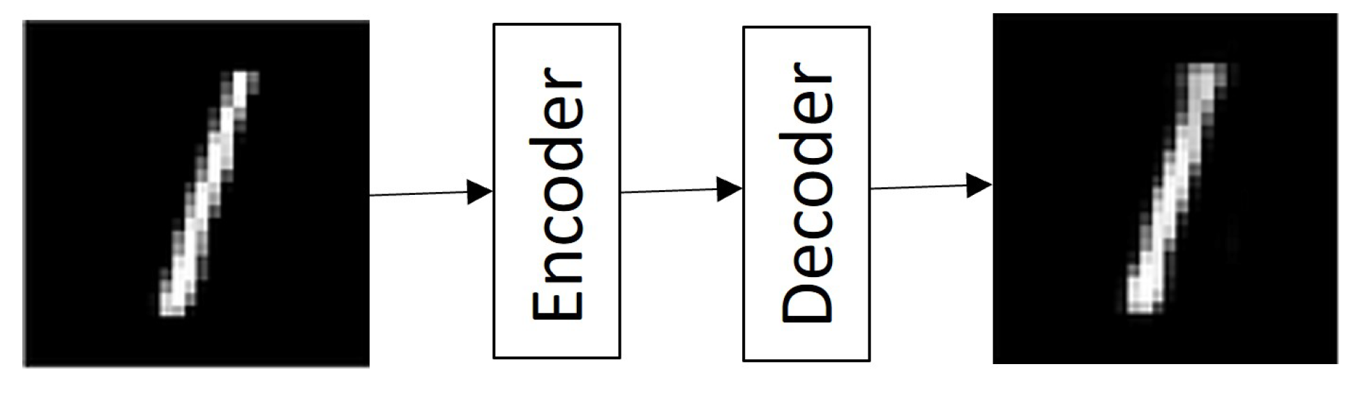
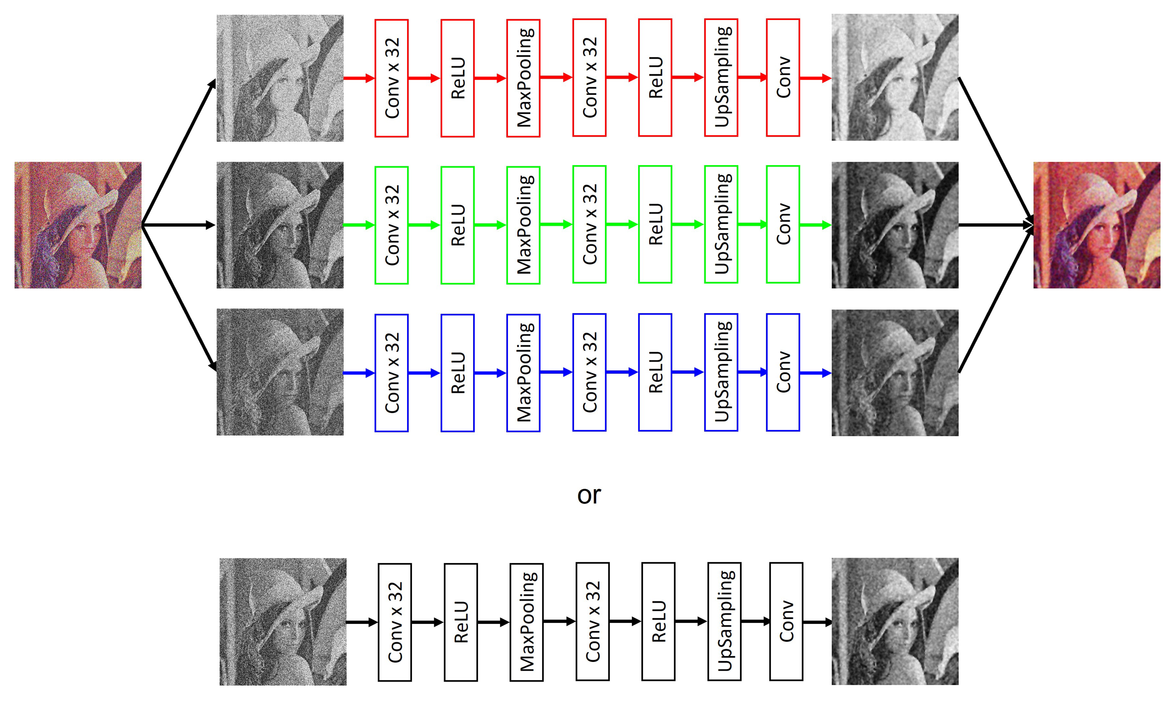
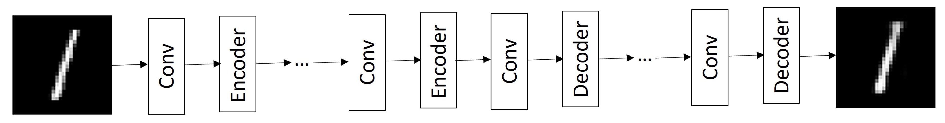
- The Vanilla Autoencoder (VA) comprises only three layers: the encoding layer, in charge of reducing the dimensions of the input information; the hidden layer, better known as latent space, in which are the representations of all characteristics learned by the network; and the decoding layer, which is in charge of restoring the information to its original input dimensions, as shown in Figure 1 [23].
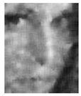
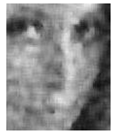
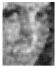
- The Denoising Autoencoder (DA) is a robust modification of Conv AE that changes the input data preparation. The information the autoencoder is trained in is divided into two groups: original and corrupted. In order for the autoencoder to learn to denoise an image, the corrupted information is sent to the input of the network to be processed. Once the information is in the output, it is compared with the original [25]. This type of autoencoder is capable of generating clean images from noisy images, ignoring the type of noise present as well as the density in which the image was affected.
3. Proposed Model
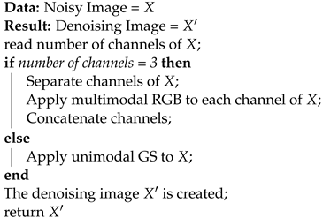
| Algorithm 1: Process image using DVA. |
 |
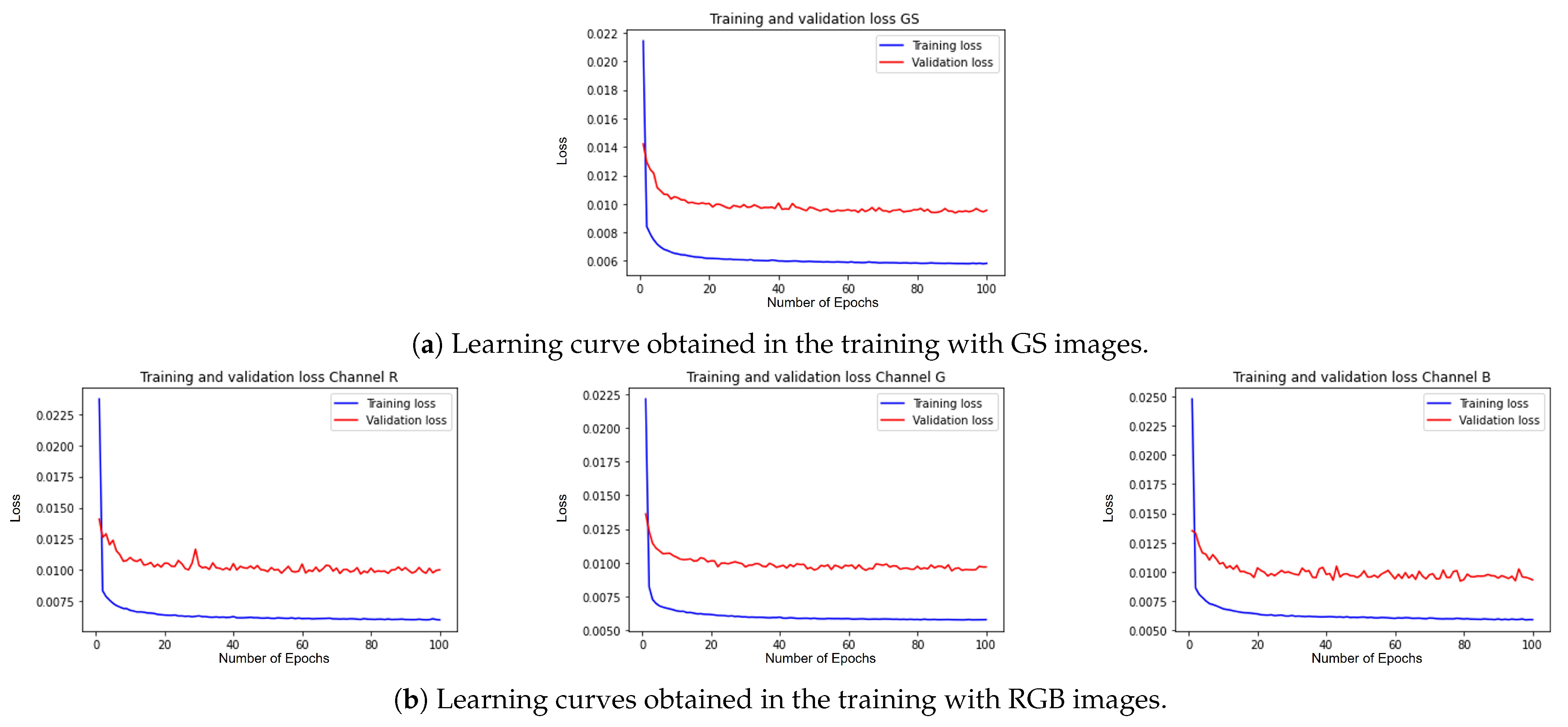
Network Training
4. Experimental Results
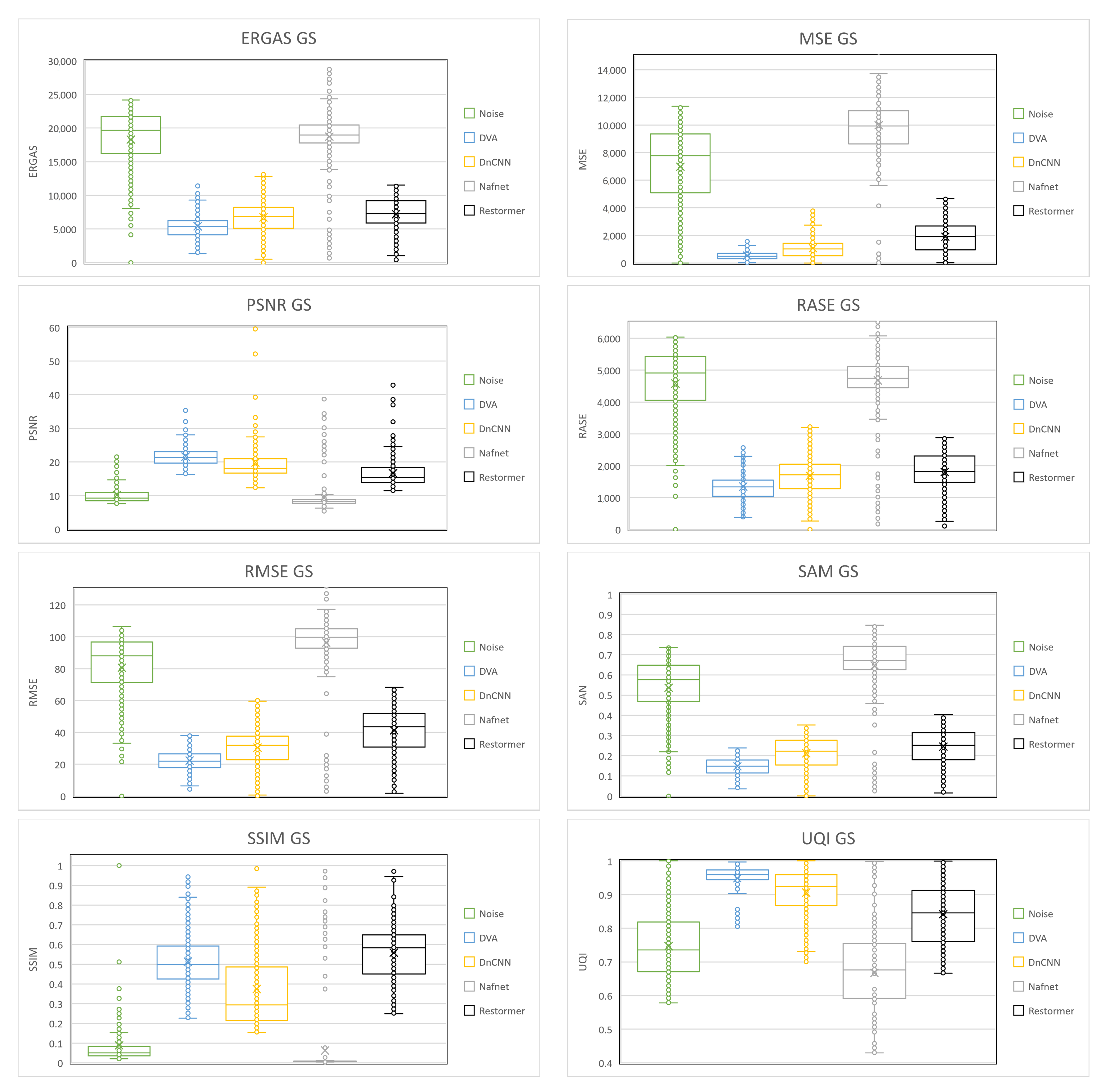
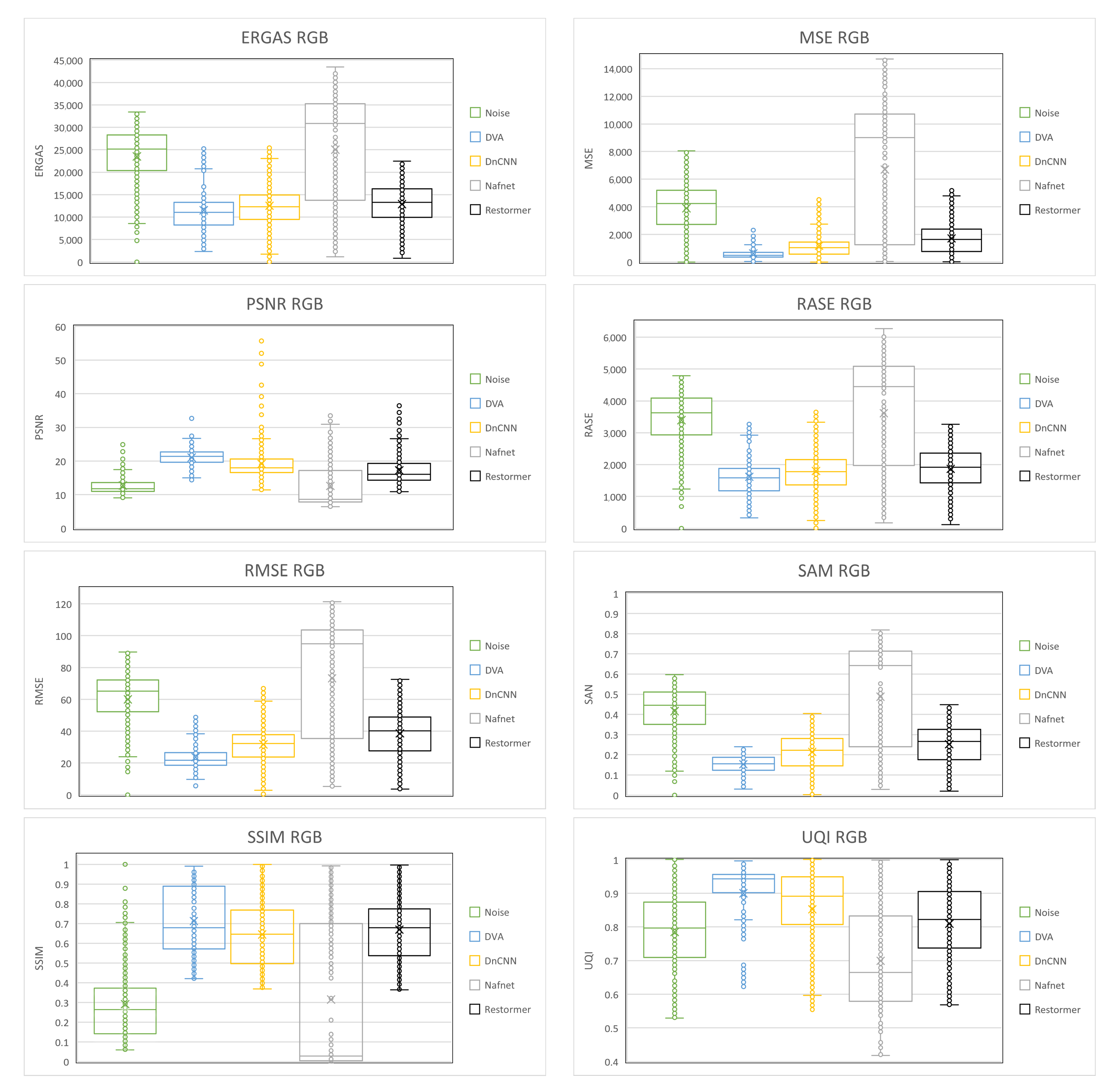
- Mean Square Error (MSE): Calculate the mean of the differences between the original images and the processed images squared.where x and y are the images to compare, is the coordinates of the pixel, and M and N are the size of the images.
- Root Mean Squared Error (RMSE): Commonly used to compare the difference between the original images and the processed images by directly computing the variation in pixel values [27].
- Erreur Relative Globale Adimensionnelle de Synthèse (ERGAS): Used to compute the quality of the processed images in terms of normalized average error of each band of processed image [28].where is the ratio of pixel between hue and light, n is the number of bands, and is the mean of the ith band.
- Peak Signal-to-Noise Ratio (PSNR): A widely used metric that is computed by the number of gray levels in the image divided by the corresponding pixels in the original images and the processed images [29].where b is the number of the bits in the image.
- Relative Average Spectral Error (RASE): Characterizes the average performance of a method in the considered spectral bands [30].where is the mean radiance of the n spectral bands, and represents ith band of the image.
- Spectral Angle Mapper (SAM): Computes the spectral angle between the pixel, the vector of the original images, and the processed images [31].
- Structural Similarity Index (SSIM): Used to compare the local patterns of pixel intensities between the original images and the processed images [32].where and are the mean of the images, respectively; is the covariance between the images to compare; and are two variables to stabilize the division with low denominators; L is the dynamic range of the pixel values; ; and .
- Universal Quality Image Index (UQI): Used to calculate the amount of transformation of relevant data from the original images into the processed images [33].
5. Conclusions
Author Contributions
Funding
Institutional Review Board Statement
Informed Consent Statement
Data Availability Statement
Acknowledgments
Conflicts of Interest
References
- Limshuebchuey, A.; Duangsoithong, R.; Saejia, M. Comparison of Image Denoising using Traditional Filter and Deep Learning Methods. In Proceedings of the 2020 17th International Conference on Electrical Engineering/Electronics, Computer, Telecommunications and Information Technology (ECTI-CON), Online, 24–27 June 2020; pp. 193–196. [Google Scholar]
- Ajay, K.B.; Brijendra, K.J. A Review Paper: Noise Models in Digital Image Processing. Comput. Res. Repos. 2015, 6, 63–75. [Google Scholar]
- Verma, R.; Ali, J. A comparative study of various types of image noise and efficient noise removal techniques. Int. J. Adv. Res. Comput. Sci. Softw. Eng. 2013, 3, 617–622. [Google Scholar]
- Tian, C.; Fei, L.; Zheng, W.; Xu, Y.; Zuo, W.; Lin, C.W. Deep Learning on Image Denoising: An Overview; Elsevier: Amsterdam, The Netherlands, 2020; pp. 1–39. [Google Scholar]
- Liu, W.; Wang, Z.; Liu, X.; Zeng, N.; Liu, Y.; Alsaadi, F.E. A survey of deep neural network architectures and their applications. Neurocomputing 2017, 234, 11–26. [Google Scholar] [CrossRef]
- Agarwal, S.; Agarwal, A.; Deshmukh, M. Denoising Images with Varying Noises Using Autoencoders. In Proceedings of the Computer Vision and Image Processing: 4th International Conference, CVIP 2019, Jaipur, India, 27–29 September 2019; Volume 1148, pp. 3–14. [Google Scholar]
- Dong, L.F.; Gan, Y.Z.; Mao, X.L. Learning Deep Representations Using Convolutional Auto-Encoders with Symmetric Skip Connections. In Proceedings of the 2018 IEEE International Conference on Acoustics, Speech and Signal Processing (ICASSP), Calgary, AB, Canada, 15–20 April 2018; pp. 3006–3010. [Google Scholar]
- Holden, D.; Saito, J.; Komura, T. Learning Motion Manifolds with Convolutional Autoencoders. Assoc. Comput. Mach. 2015, 18, 1–4. [Google Scholar] [CrossRef]
- Zhang, K.; Zuo, W.; Chen, Y. Beyond a Gaussian Denoiser: Residual Learning of Deep CNN for Image Denoising. IEEE Trans. Image Process. 2017, 26, 3142–3155. [Google Scholar] [CrossRef]
- Chen, L.; Chu, X.; Zhang, X.; Sun, J. Simple Baselines for Image Restoration. arXiv 2022, arXiv:2204.04676v4. [Google Scholar]
- Zamir, S.W.; Arora, A.; Khan, S. Restormer: Efficient Transformer for High-Resolution Image Restoration. arXiv 2021, arXiv:2111.09881. [Google Scholar]
- Xiaojun, C.; Ren, P.; Xu, P. A Comprehensive Survey of Scene Graphs: Generation and Application. IEEE Trans. Pattern Anal. Mach. Intell. 2022, 45, 22359232. [Google Scholar]
- Steffen, S.; Adrian, S.; Kendra, B. Image Processing of Multi-Phase Images Obtained via X-ray Microtomography: A Review; American Geophysical Union: Washington, DC, USA, 2014. [Google Scholar]
- Balafar, M.; Ramli, M. Review of brain mri image segmentation methods. Artif. Intell. 2010, 33, 261–274. [Google Scholar] [CrossRef]
- Mario, V.; Francesco, M.; Giovanni, A. Adaptive Image Contrast Enhancement by Computing Distances into a 4-Dimensional Fuzzy Unit Hypercube; IEEE: Washington, DC, USA, 2017; pp. 26922–26931. [Google Scholar]
- Diwakar, M.; Kumar, M. A review on ct image noise and its denoising. Biomed. Process. Control 2017, 42, 73–88. [Google Scholar] [CrossRef]
- Chollet, F. Deep Learning with Python; Simon & Schuster: New York, NY, USA, 2018; p. 384. [Google Scholar]
- Zhang, L.; Chang, X.; Liu, J.; Luo, M.; Li, Z.; Yao, L.; Hauptmann, A. TN-ZSTAD: Transferable Network for Zero-Shot Temporal Activity Detection; IEEE: Washington, DC, USA, 2023; pp. 3848–3861. [Google Scholar]
- Aurelien, G. Hands-On Machine Learning with Scikit-Learn and TensorFlow Concepts; O’Reilly Media, Inc.: Sebastopol, CA, USA, 2017; p. 856. [Google Scholar]
- Gulli, A. Deep Learning with Keras; Packt Publishing Ltd.: Birmingham, UK, 2017; p. 318. [Google Scholar]
- Karatsiolis, S.; Schizas, C. Conditional Generative Denoising Autoencoder; IEEE: Washington, DC, USA, 2020; pp. 4117–4129. [Google Scholar]
- Majumdar, A. Blind Denoising Autoencoder. IEEE Trans. Neural Netw. Learn. Syst. 2019, 30, 312–317. [Google Scholar] [CrossRef] [PubMed]
- Hinton, G.E.; Salakhutdinov, R.R. Reducing the dimensionality of data with neural networks. Science 2006, 313, 504–507. [Google Scholar] [CrossRef] [PubMed]
- Leonard, M. Deep Learning Nanodegree Foundation Course; LectureNotes in Autoencoders; Udacity: Emeryville, CA, USA, 2018. [Google Scholar]
- Vincent, P.; Larochelle, H.; Bengio, Y. Extracting and composing robust features with denoising autoencoders. In Proceedings of the 25th International Conference on Machine Learning, Helsinki, Finland, 5–9 July 2008; pp. 1096–1103. [Google Scholar]
- Bojan, T. “1 Million Faces”. Kaggle. Available online: https://www.kaggle.com/competitions/deepfake-detection-challenge/discussion/121173 (accessed on 20 February 2023).
- Zoran, L.F. Quality Evaluation of Multiresolution Remote Sensing Image Fusion. UPB Sci. Bull. 2009, 71, 38–52. [Google Scholar]
- Du, Q.; Younan, N.H.; King, R. On the performance evaluation of pan-sharpening techniques. IEEE Remote Sens. 2007, 4, 518–522. [Google Scholar] [CrossRef]
- Naidu, V.P.S. Discrete Cosine Transform-based Image Fusion. Navig. Signal Process. 2010, 60, 33–45. [Google Scholar]
- Shailesh, P.; Rajesh, T. Implementation and comparative quantitative assessment of different multispectral image pansharpening approaches. Signal Image Process. Int. J. 2015, 35–48. [Google Scholar] [CrossRef]
- Alparone, L.; Wald, L.; Chanussot, J. Comparison of Pansharpening Algorithms: Outcome of the 2006 GRS-S Data-Fusion Contest. IEEE Trans. Geosci. Remote Sens. 2007, 45, 3012–3021. [Google Scholar] [CrossRef]
- Wang, Z.; Bovik, A.C.; Sheikh, H.R. Image Quality Assessment from Error Visibility to Structural Similarity. IEEE Trans. Image Process. 2004, 13, 600–612. [Google Scholar] [CrossRef] [PubMed]
- Alparone, L.; Aiazzi, B.; Baronti, S. Multispectral and Panchromatic Data Fusion Assessment Without Reference. Photogramm. Eng. Remote Sens. 2008, 74, 193–200. [Google Scholar] [CrossRef]
- Zhang, K.; Ren, W.; Luo, W. Deep Image Deblurring: A Survey; Springer: Berlin/Heidelberg, Germany, 2022; pp. 2103–2130. [Google Scholar]
- Hoßfeld, T.; Heegaard, P.E.; Varela, M. Qoe beyond the Mos: An In-Depth Look at Qoe via Better Metrics and Their Relation to Mos; Springer: Berlin/Heidelberg, Germany, 2016. [Google Scholar]
- Yan, C.; Chang, X.; Li, Z. ZeroNAS: Differentiable Generative Adversarial Networks Search for Zero-Shot Learning; IEEE: Washington, DC, USA, 2022; pp. 9733–9740. [Google Scholar]


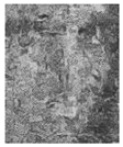
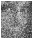
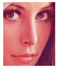
Original GS Image | ||||||
|---|---|---|---|---|---|---|
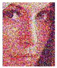
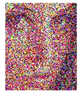
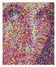
| Noisy Images | ||||||
 | 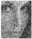 | 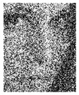 | 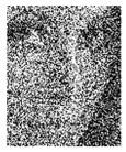 | 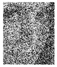 | 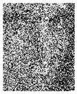 |  |
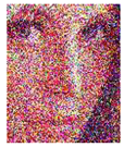
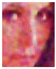
| DVA results | ||||||
 |  |  |  |  |  |  |
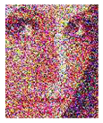
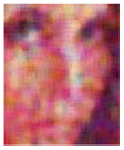
| DnCNN results | ||||||
 |  |  |  |  |  |  |
| Restormer results | ||||||
 |  |  |  |  |  |  |
| Nafnet results | ||||||
 |  |  |  |  |  |  |
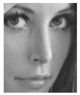
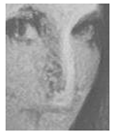
Original RGB Image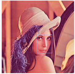 | ||||||
|---|---|---|---|---|---|---|
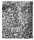
| Noisy Images | ||||||
 |  |  |  |  |  |  |
| DVA results | ||||||
 |  |  |  |  |  |  |
| DnCNN results | ||||||
 |  |  |  |  |  |  |
| Restormer results | ||||||
 |  |  |  |  |  |  |
| Nafnet results | ||||||
 |  |  |  |  |  |  |
| GS Image | Density | Noisy Image | DVA | DnCNN | Restormer | Nafnet |
|---|---|---|---|---|---|---|
| Airplane GS | 0 | inf | 26.545 | 71.197 | 36.987 | 32.961 |
| 0.10 | 11.859 | 23.729 | 22.305 | 22.137 | 10.312 | |
| 0.15 | 10.610 | 23.014 | 20.097 | 20.818 | 7.995 | |
| 0.20 | 9.841 | 22.378 | 18.705 | 20.128 | 8.717 | |
| 0.30 | 8.896 | 20.938 | 16.859 | 19.132 | 9.407 | |
| 0.40 | 8.338 | 20.474 | 15.833 | 18.476 | 8.043 | |
| 0.50 | 7.959 | 19.312 | 15.109 | 17.937 | 7.823 | |
| Baboon GS | 0 | inf | 17.478 | 33.966 | 26.414 | 10.021 |
| 0.10 | 11.298 | 19.010 | 20.203 | 17.560 | 8.926 | |
| 0.15 | 10.221 | 18.103 | 19.277 | 16.634 | 9.159 | |
| 0.20 | 9.592 | 18.596 | 18.676 | 16.003 | 8.892 | |
| 0.30 | 8.824 | 18.222 | 17.654 | 15.294 | 8.761 | |
| 0.40 | 8.377 | 17.913 | 16.975 | 14.827 | 8.840 | |
| 0.50 | 8.066 | 17.702 | 16.480 | 14.476 | 8.861 | |
| Barbara GS | 0 | inf | 23.640 | 39.198 | 32.285 | 8.417 |
| 0.10 | 11.469 | 21.795 | 21.669 | 17.472 | 8.846 | |
| 0.15 | 10.336 | 21.309 | 20.191 | 16.120 | 9.119 | |
| 0.20 | 9.673 | 20.119 | 19.171 | 15.245 | 8.514 | |
| 0.30 | 8.837 | 20.160 | 17.726 | 14.150 | 8.054 | |
| 0.40 | 8.330 | 19.672 | 16.762 | 13.450 | 8.051 | |
| 0.50 | 8.029 | 18.975 | 16.241 | 13.083 | 8.124 | |
| Cablecar GS | 0 | inf | 25.853 | 67.160 | 36.974 | 31.302 |
| 0.10 | 12.069 | 22.686 | 20.751 | 17.113 | 7.295 | |
| 0.15 | 10.800 | 22.084 | 19.047 | 15.690 | 6.993 | |
| 0.20 | 9.951 | 21.032 | 17.636 | 14.640 | 7.270 | |
| 0.30 | 8.910 | 20.558 | 15.981 | 13.406 | 7.123 | |
| 0.40 | 8.290 | 19.643 | 14.945 | 12.686 | 6.887 | |
| 0.50 | 7.872 | 18.765 | 14.216 | 12.198 | 6.826 | |
| Goldhill GS | 0 | inf | 27.997 | 52.056 | 39.720 | 33.700 |
| 0.10 | 11.595 | 24.867 | 22.684 | 17.541 | 7.818 | |
| 0.15 | 10.450 | 23.896 | 20.744 | 15.958 | 8.031 | |
| 0.20 | 9.722 | 23.346 | 19.390 | 14.898 | 7.954 | |
| 0.30 | 8.857 | 22.313 | 17.686 | 13.676 | 7.718 | |
| 0.40 | 8.335 | 21.505 | 16.637 | 12.948 | 7.716 | |
| 0.50 | 7.971 | 20.774 | 15.874 | 12.460 | 7.640 | |
| Lenna GS | 0 | inf | 30.196 | 72.566 | 38.527 | 35.414 |
| 0.10 | 11.383 | 24.344 | 23.652 | 18.997 | 8.645 | |
| 0.15 | 10.284 | 23.743 | 21.720 | 17.578 | 9.051 | |
| 0.20 | 9.619 | 22.941 | 20.332 | 16.749 | 8.815 | |
| 0.30 | 8.825 | 21.901 | 18.565 | 15.609 | 8.394 | |
| 0.40 | 8.350 | 21.074 | 17.501 | 14.968 | 8.531 | |
| 0.50 | 8.049 | 20.650 | 16.899 | 14.571 | 8.566 | |
| Mondrian GS | 0 | inf | 20.117 | 59.524 | 31.921 | 30.121 |
| 0.10 | 12.534 | 19.672 | 18.876 | 16.526 | 5.621 | |
| 0.15 | 11.070 | 20.003 | 17.094 | 14.994 | 5.678 | |
| 0.20 | 10.075 | 19.170 | 15.790 | 13.970 | 5.581 | |
| 0.30 | 8.842 | 18.086 | 14.121 | 12.713 | 5.426 | |
| 0.40 | 8.094 | 16.578 | 13.068 | 11.969 | 5.475 | |
| 0.50 | 7.581 | 16.204 | 12.323 | 11.446 | 5.447 | |
| Peppers GS | 0 | inf | 25.598 | 62.046 | 38.161 | 34.348 |
| 0.10 | 11.479 | 24.303 | 23.371 | 18.504 | 8.340 | |
| 0.15 | 10.353 | 23.010 | 21.187 | 16.975 | 8.754 | |
| 0.20 | 9.667 | 22.402 | 19.909 | 16.064 | 8.560 | |
| 0.30 | 8.829 | 21.752 | 18.033 | 14.940 | 8.160 | |
| 0.40 | 8.363 | 21.193 | 17.149 | 14.347 | 8.159 | |
| 0.50 | 8.023 | 20.383 | 16.363 | 13.838 | 8.258 |
| RGB Image | Density | Noisy Image | DVA | DnCNN | Restormer | Nafnet |
|---|---|---|---|---|---|---|
| Airplane RGB | 0 | inf | 26.215 | 55.638 | 36.502 | 32.961 |
| 0.10 | 14.576 | 24.082 | 22.852 | 23.812 | 10.312 | |
| 0.15 | 13.342 | 23.365 | 20.843 | 22.569 | 7.995 | |
| 0.20 | 12.526 | 22.461 | 19.449 | 21.548 | 8.717 | |
| 0.30 | 11.525 | 21.899 | 17.694 | 20.237 | 9.407 | |
| 0.40 | 10.922 | 21.228 | 16.665 | 19.421 | 8.043 | |
| 0.50 | 10.503 | 19.762 | 15.926 | 18.798 | 7.823 | |
| Baboon RGB | 0 | inf | 21.614 | 25.291 | 23.442 | 10.021 |
| 0.10 | 14.043 | 19.171 | 19.781 | 17.699 | 8.926 | |
| 0.15 | 12.981 | 18.895 | 18.917 | 16.758 | 9.159 | |
| 0.20 | 12.314 | 18.704 | 18.245 | 16.122 | 8.892 | |
| 0.30 | 11.488 | 18.475 | 17.324 | 15.377 | 8.761 | |
| 0.40 | 10.961 | 18.144 | 16.665 | 14.828 | 8.840 | |
| 0.50 | 10.653 | 17.850 | 16.297 | 14.521 | 8.861 | |
| Barbara RGB | 0 | inf | 27.412 | 39.115 | 31.285 | 29.037 |
| 0.10 | 14.269 | 21.742 | 21.857 | 18.259 | 16.990 | |
| 0.15 | 13.134 | 21.271 | 20.416 | 17.002 | 8.152 | |
| 0.20 | 12.425 | 21.059 | 19.426 | 16.145 | 8.285 | |
| 0.30 | 11.553 | 20.518 | 18.128 | 15.050 | 7.846 | |
| 0.40 | 11.033 | 20.157 | 17.285 | 14.348 | 7.867 | |
| 0.50 | 10.663 | 19.707 | 16.726 | 13.854 | 8.348 | |
| Cablecar RGB | 0 | inf | 22.794 | 52.131 | 34.426 | 30.961 |
| 0.10 | 14.652 | 21.977 | 20.843 | 18.035 | 10.152 | |
| 0.15 | 13.293 | 21.563 | 18.983 | 16.419 | 7.520 | |
| 0.20 | 12.411 | 20.120 | 17.758 | 15.419 | 7.403 | |
| 0.30 | 11.284 | 20.164 | 16.115 | 14.106 | 6.997 | |
| 0.40 | 10.612 | 19.757 | 15.146 | 13.304 | 6.878 | |
| 0.50 | 10.143 | 19.036 | 14.452 | 12.725 | 6.985 | |
| Goldhill RGB | 0 | inf | 32.649 | 51.974 | 36.456 | 32.535 |
| 0.10 | 14.323 | 23.988 | 22.748 | 19.003 | 8.023 | |
| 0.15 | 13.149 | 23.362 | 20.968 | 17.287 | 8.134 | |
| 0.20 | 12.392 | 23.037 | 19.680 | 16.187 | 7.666 | |
| 0.30 | 11.501 | 22.456 | 18.193 | 14.890 | 7.438 | |
| 0.40 | 10.927 | 21.856 | 17.201 | 14.020 | 7.585 | |
| 0.50 | 10.558 | 21.181 | 16.556 | 13.482 | 7.853 | |
| Lenna RGB | 0 | inf | 28.446 | 33.758 | 32.538 | 31.828 |
| 0.10 | 14.368 | 23.799 | 23.141 | 21.068 | 21.847 | |
| 0.15 | 13.249 | 23.332 | 21.434 | 19.475 | 10.198 | |
| 0.20 | 12.496 | 22.966 | 20.143 | 18.344 | 8.230 | |
| 0.30 | 11.611 | 22.467 | 18.691 | 17.022 | 8.185 | |
| 0.40 | 11.084 | 21.703 | 17.758 | 16.191 | 8.164 | |
| 0.50 | 10.707 | 21.152 | 17.063 | 15.629 | 8.189 | |
| Mondrian RGB | 0 | inf | 17.688 | 36.324 | 29.113 | 28.609 |
| 0.10 | 14.728 | 16.729 | 17.404 | 16.621 | 15.873 | |
| 0.15 | 13.072 | 16.465 | 15.700 | 14.978 | 14.440 | |
| 0.20 | 11.976 | 15.927 | 14.560 | 13.850 | 13.526 | |
| 0.30 | 10.568 | 15.098 | 13.054 | 12.432 | 12.291 | |
| 0.40 | 9.690 | 14.841 | 12.086 | 11.545 | 11.420 | |
| 0.50 | 9.070 | 15.039 | 11.391 | 10.917 | 10.330 | |
| Peppers RGB | 0 | inf | 33.057 | 48.801 | 34.615 | 32.112 |
| 0.10 | 14.519 | 24.496 | 22.653 | 19.361 | 19.103 | |
| 0.15 | 13.324 | 23.756 | 20.752 | 17.669 | 17.418 | |
| 0.20 | 12.540 | 23.349 | 19.468 | 16.594 | 16.102 | |
| 0.30 | 11.565 | 22.606 | 17.837 | 15.310 | 7.490 | |
| 0.40 | 10.974 | 21.553 | 16.868 | 14.491 | 7.657 | |
| 0.50 | 10.569 | 20.784 | 16.179 | 13.942 | 7.667 |
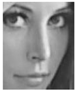
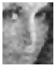
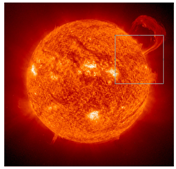 |  | ||||
| Sun 2100 × 2034 | |||||
 |  | 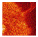 |  |  |  |
 |  |  |  |  |  |
| ERGAS = 5169.806 | ERGAS = 10,965.422 | ERGAS = 13,395.159 | ERGAS = 15,276.500 | ERGAS = 17,736.873 | ERGAS = 18,296.674 |
| MSE = 21.131 | MSE = 124.536 | MSE = 249.594 | MSE = 380.183 | MSE = 567.533 | MSE = 699.633 |
| PSNR = 34.882 | PSNR = 27.178 | PSNR = 24.158 | PSNR = 22.331 | PSNR = 20.591 | PSNR = 19.682 |
| RASE = 0 | RASE = 1498.244 | RASE = 1902.722 | RASE = 2190.058 | RASE = 2530.487 | RASE = 2639.515 |
| RMSE = 4.597 | RMSE = 11.160 | RMSE = 15.799 | RMSE = 19.498 | RMSE = 23.823 | RMSE = 26.451 |
| SAM = 0.072 | SAM = 0.273 | SAM = 0.390 | SAM = 0.448 | SAM = 0.489 | SAM = 0.523 |
| SSIM = 0.994 | SSIM = 0.964 | SSIM = 0.926 | SSIM = 0.896 | SSIM = 0.867 | SSIM = 0.842 |
| UQI = 0.782 | UQI = 0.558 | UQI = 0.512 | UQI = 0.499 | UQI = 0.490 | UQI = 0.484 |
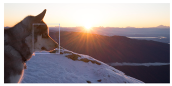
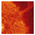
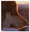
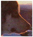
| Dog 6000 × 2908 | |||||
 |  |  |  |  |  |
 |  |  |  |  |  |
| ERGAS = 5624.483 | ERGAS = 11,456.096 | ERGAS = 10,623.462 | ERGAS = 10,393.671 | ERGAS = 9919.464 | ERGAS = 10,406.266 |
| MSE = 217.856 | MSE = 362.834 | MSE = 441.465 | MSE = 566.388 | MSE = 610.187 | MSE = 763.037 |
| PSNR = 24.749 | PSNR = 22.534 | PSNR = 21.682 | PSNR = 20.6 | PSNR = 20.276 | PSNR = 19.305 |
| RASE = 806.958 | RASE = 1652.544 | RASE = 1530.997 | RASE = 1496.294 | RASE = 1427.232 | RASE = 1496.917 |
| RMSE = 14.76 | RMSE = 19.048 | RMSE = 21.011 | RMSE = 23.799 | RMSE = 24.702 | RMSE = 27.623 |
| SAM = 0.022 | SAM = 0.078 | SAM = 0.089 | SAM = 0.099 | SAM = 0.113 | SAM = 0.131 |
| SSIM = 0.936 | SSIM = 0.773 | SSIM = 0.711 | SSIM = 0.665 | SSIM = 0.623 | SSIM = 0.588 |
| UQI = 0.986 | UQI = 0.936 | UQI = 0.948 | UQI = 0.953 | UQI = 0.956 | UQI = 0.951 |
Disclaimer/Publisher’s Note: The statements, opinions and data contained in all publications are solely those of the individual author(s) and contributor(s) and not of MDPI and/or the editor(s). MDPI and/or the editor(s) disclaim responsibility for any injury to people or property resulting from any ideas, methods, instructions or products referred to in the content. |
© 2023 by the authors. Licensee MDPI, Basel, Switzerland. This article is an open access article distributed under the terms and conditions of the Creative Commons Attribution (CC BY) license (https://creativecommons.org/licenses/by/4.0/).
Share and Cite
Miranda-González, A.A.; Rosales-Silva, A.J.; Mújica-Vargas, D.; Escamilla-Ambrosio, P.J.; Gallegos-Funes, F.J.; Vianney-Kinani, J.M.; Velázquez-Lozada, E.; Pérez-Hernández, L.M.; Lozano-Vázquez, L.V. Denoising Vanilla Autoencoder for RGB and GS Images with Gaussian Noise. Entropy 2023, 25, 1467. https://doi.org/10.3390/e25101467
Miranda-González AA, Rosales-Silva AJ, Mújica-Vargas D, Escamilla-Ambrosio PJ, Gallegos-Funes FJ, Vianney-Kinani JM, Velázquez-Lozada E, Pérez-Hernández LM, Lozano-Vázquez LV. Denoising Vanilla Autoencoder for RGB and GS Images with Gaussian Noise. Entropy. 2023; 25(10):1467. https://doi.org/10.3390/e25101467
Chicago/Turabian StyleMiranda-González, Armando Adrián, Alberto Jorge Rosales-Silva, Dante Mújica-Vargas, Ponciano Jorge Escamilla-Ambrosio, Francisco Javier Gallegos-Funes, Jean Marie Vianney-Kinani, Erick Velázquez-Lozada, Luis Manuel Pérez-Hernández, and Lucero Verónica Lozano-Vázquez. 2023. "Denoising Vanilla Autoencoder for RGB and GS Images with Gaussian Noise" Entropy 25, no. 10: 1467. https://doi.org/10.3390/e25101467
APA StyleMiranda-González, A. A., Rosales-Silva, A. J., Mújica-Vargas, D., Escamilla-Ambrosio, P. J., Gallegos-Funes, F. J., Vianney-Kinani, J. M., Velázquez-Lozada, E., Pérez-Hernández, L. M., & Lozano-Vázquez, L. V. (2023). Denoising Vanilla Autoencoder for RGB and GS Images with Gaussian Noise. Entropy, 25(10), 1467. https://doi.org/10.3390/e25101467