
Chaos and Thermalization in the Spin-Boson Dicke Model

 , , , , and
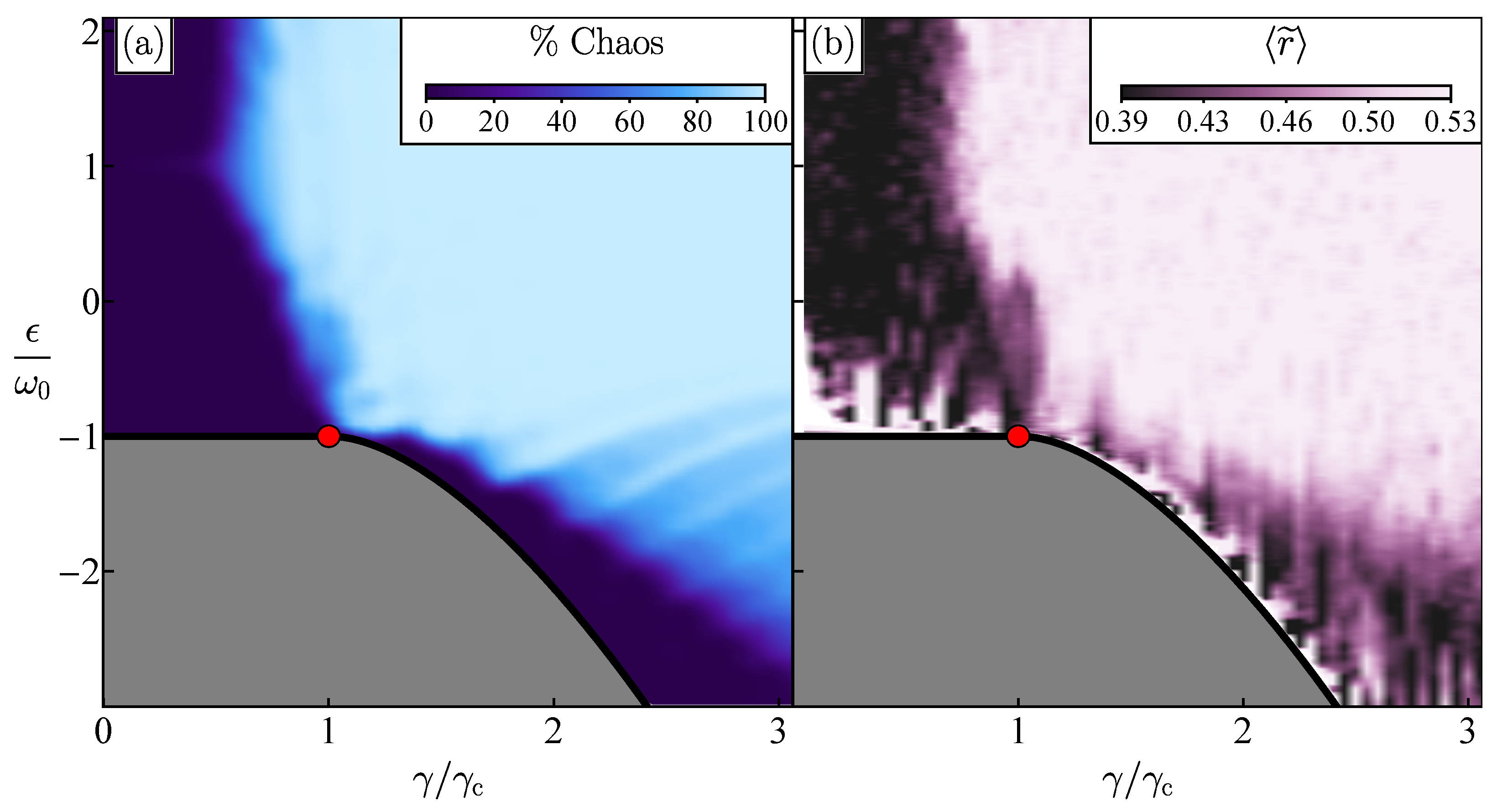
Abstract
1. Introduction
if one selects a state “at random” from an energy shell and determines, as a function of time, the probability that it lies in a “typical” subspace of the shell, the time average of this probability is liable to be much closer to the statistical expectation than is its instantaneous value, the more so the less degenerate the spectrum of the Hamiltonian.
even an initial energy eigenstate will exhibit a constant value for the observable which is very close to that predicted by the statistical theory,
2. Dicke Model
3. Chaos in the Dicke Model
4. Thermalization in the Dicke Model
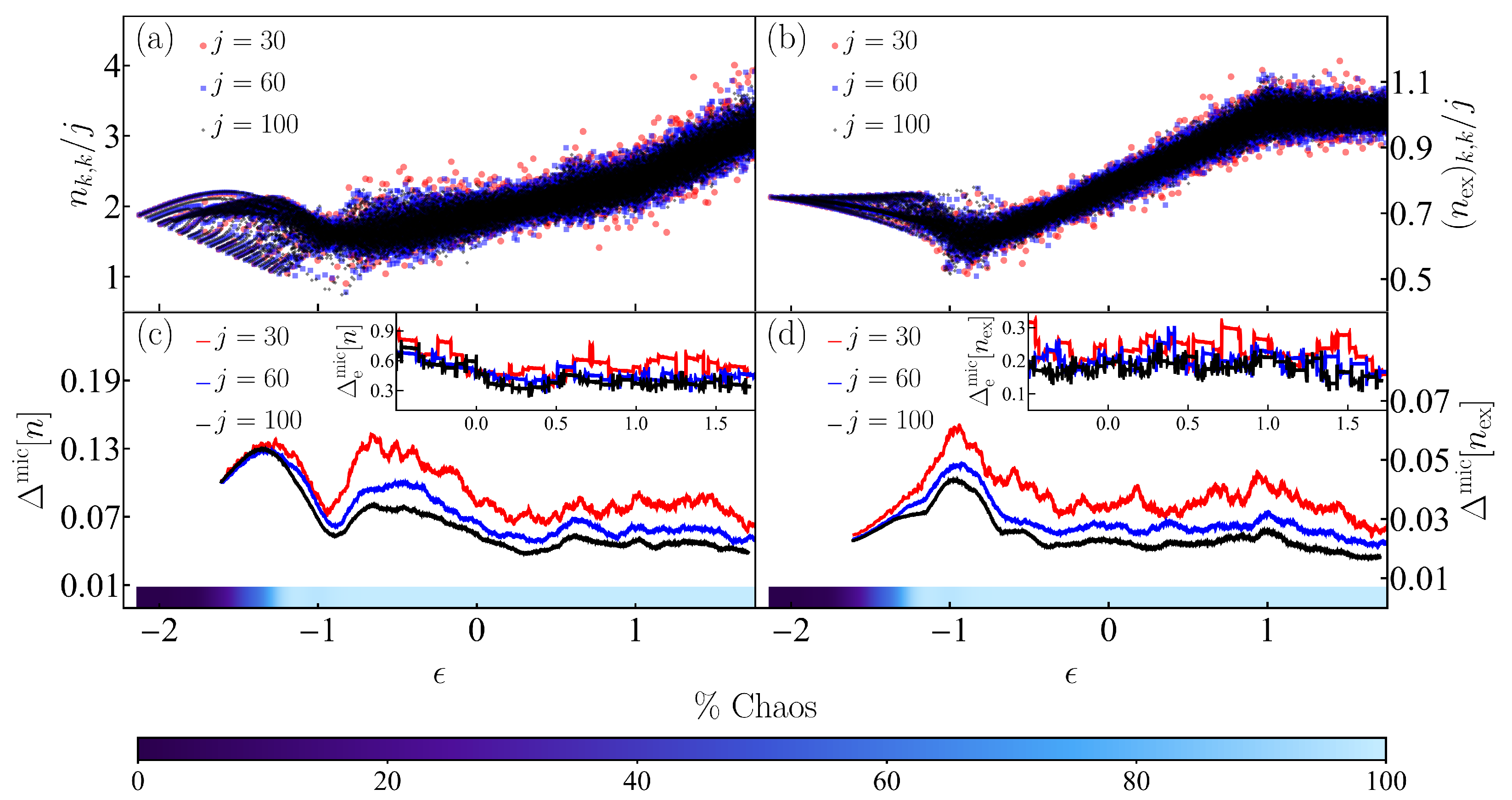
4.1. Diagonal ETH
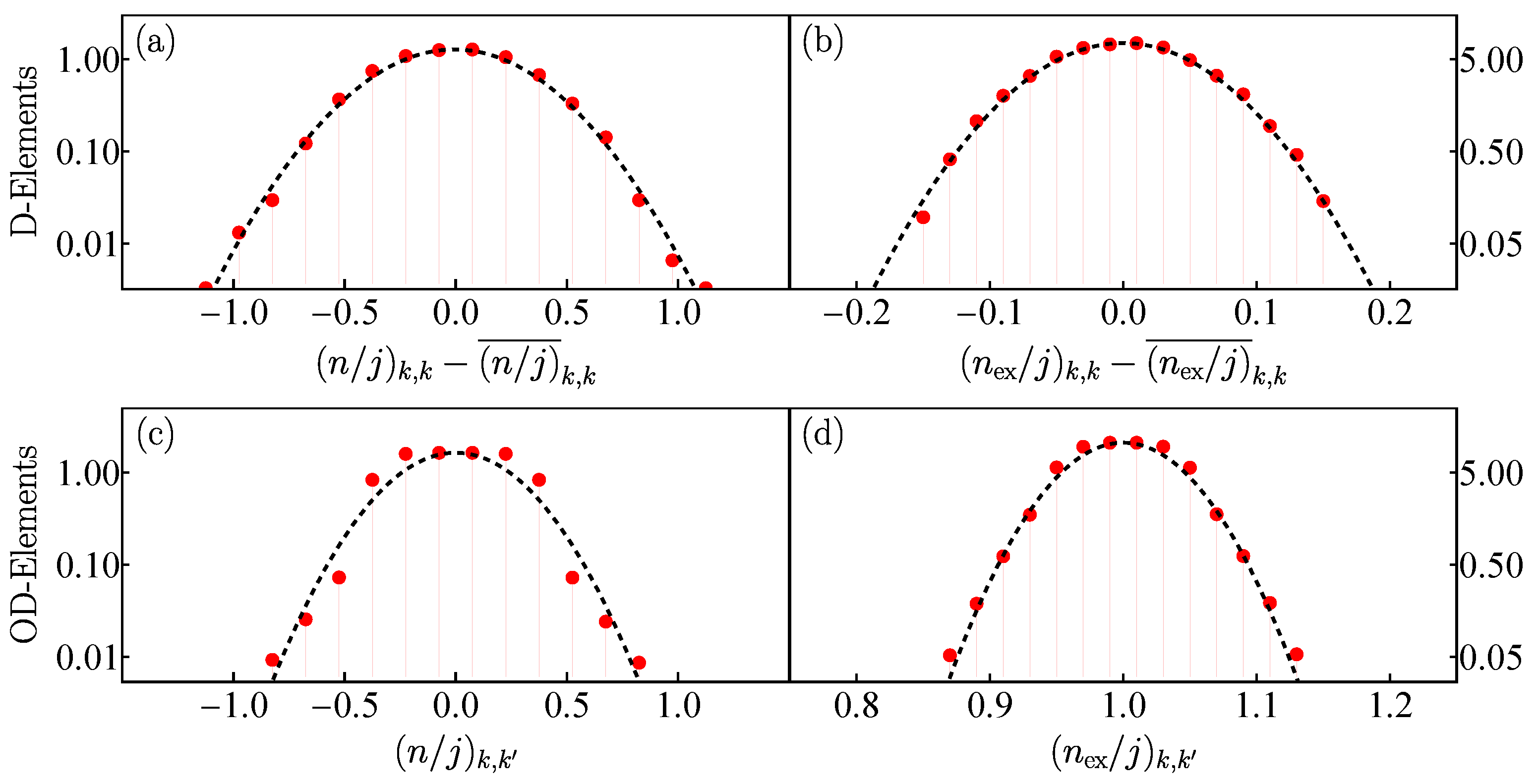
4.2. Off-Diagonal ETH
5. Entropies of the Eigenstates of the Dicke Model
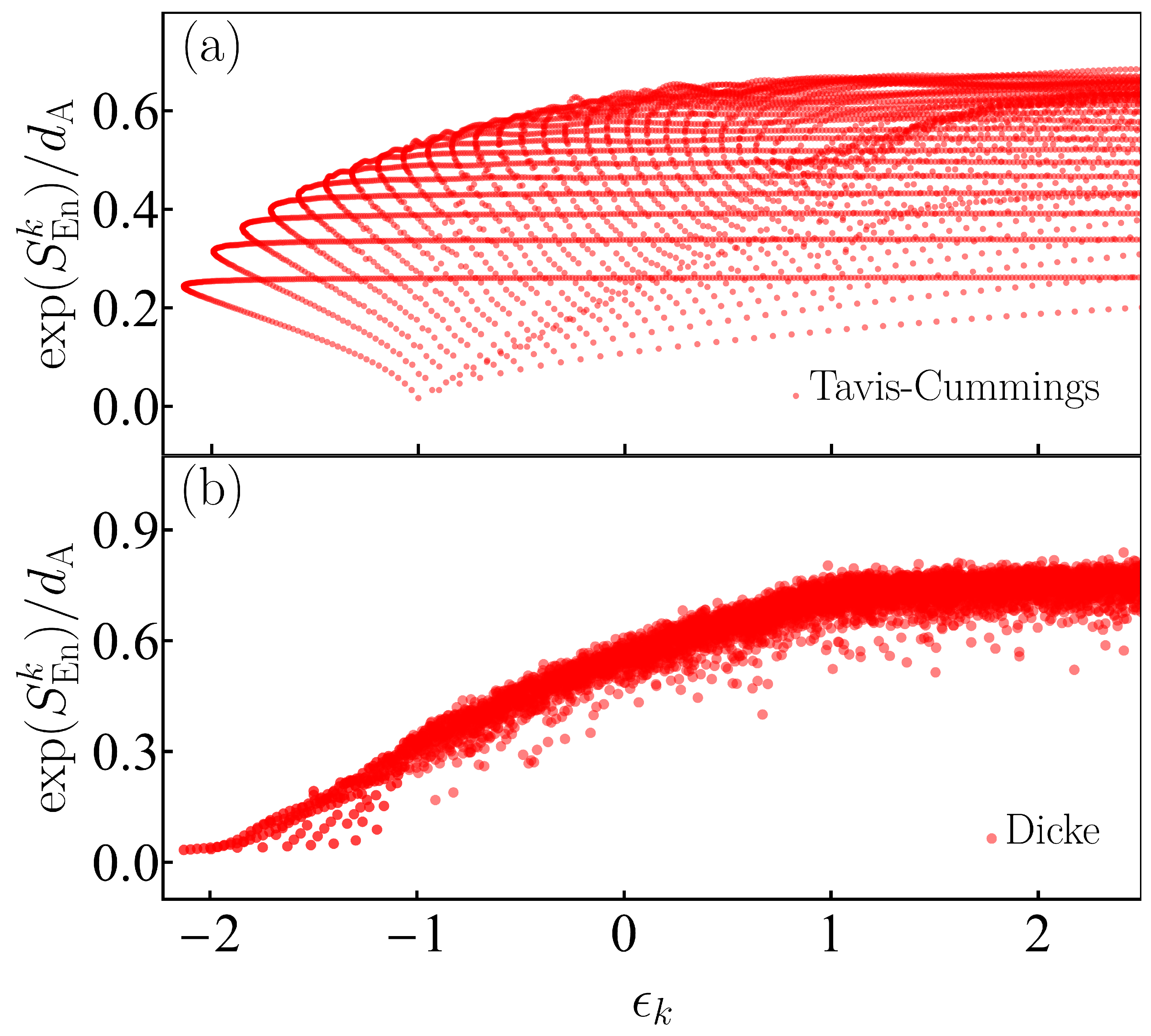
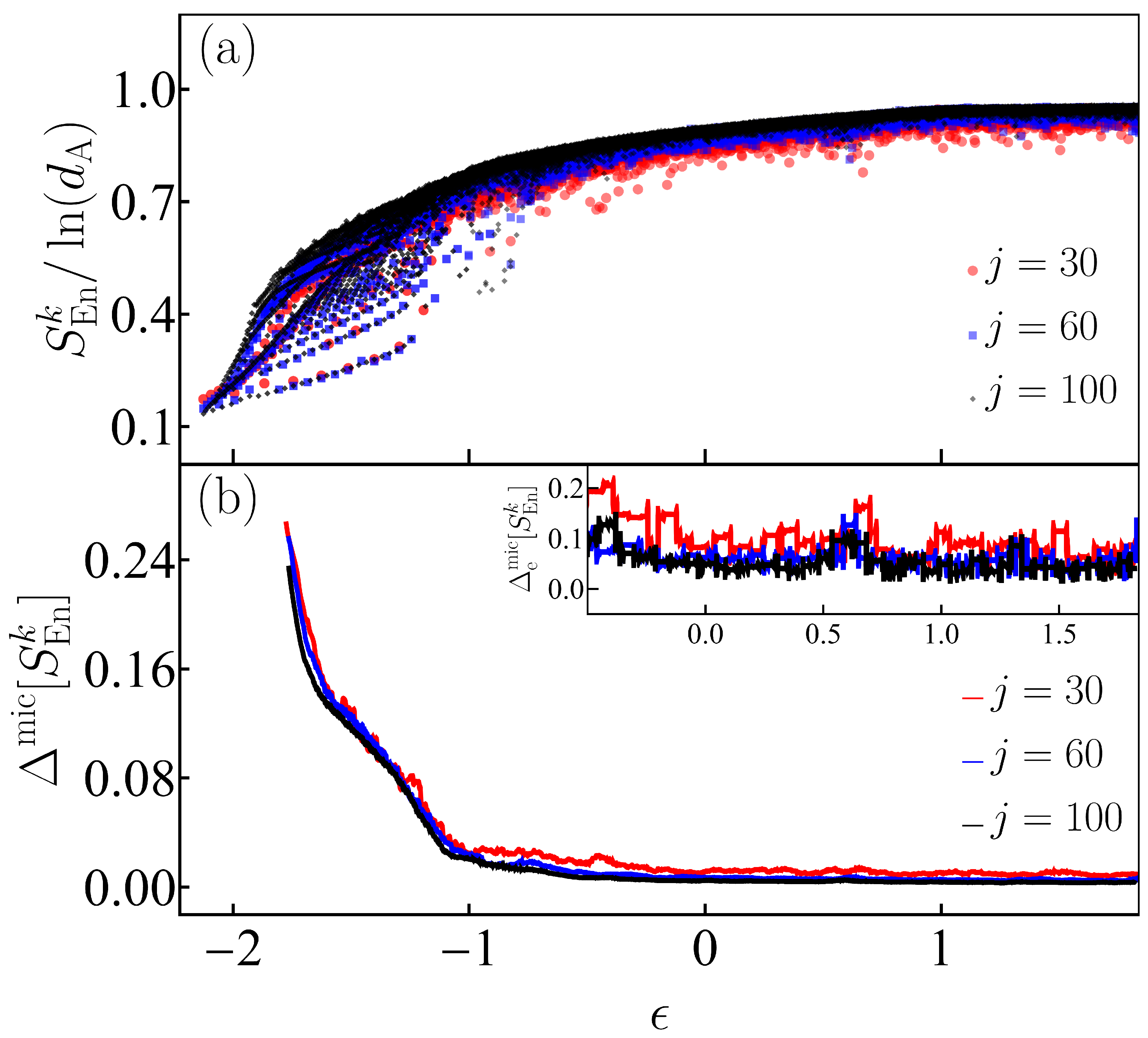
5.1. Results for the Entanglement Entropy
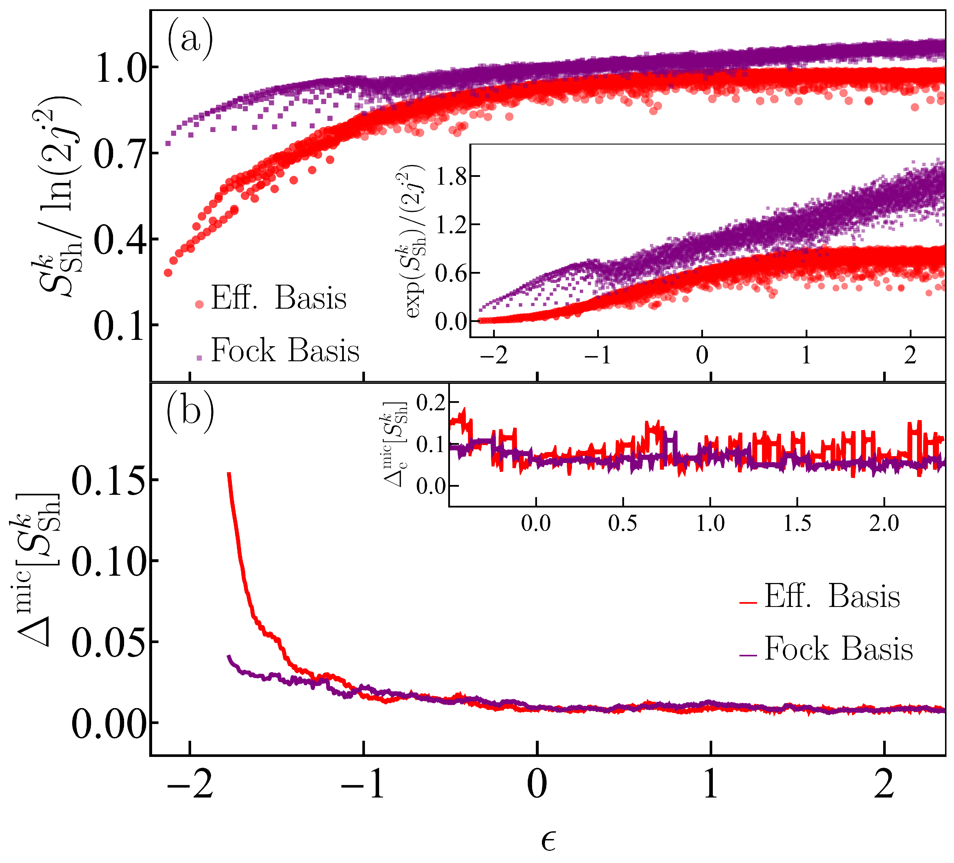
5.2. Results for the Shannon Entropy
6. Conclusions
Author Contributions
Funding
Institutional Review Board Statement
Data Availability Statement
Acknowledgments
Conflicts of Interest
Abbreviations
| ETH | eigenstate thermalization hypothesis |
| RMT | random matrix theory |
| OTOC | out-of-time-ordered correlator |
Appendix A. Diagonalization Bases
Appendix A.1. Fock Basis
Appendix A.2. Efficient Basis
Appendix A.3. Mapping from Efficient Basis to Fock Basis
Appendix B. Classical Limit of the Dicke Model
Appendix C. Quantum Entanglement
Appendix D. Integrable Dicke Model: Tavis–Cummings Model
References
- Von Neumann, J. Beweis des Ergodensatzes und des H-Theorems in der neuen Mechanik. Zeitschrift für Physik 1929, 57, 30–70. [Google Scholar] [CrossRef]
- Von Neumann, J. Proof of the ergodic theorem and the H-theorem in quantum mechanics. Eur. Phys. J. H 2010, 35, 201–237. [Google Scholar] [CrossRef]
- Goldstein, S.; Lebowitz, J.L.; Tumulka, R.; Zanghì, N. Long-time behavior of macroscopic quantum systems. Eur. Phys. J. H 2010, 35, 173–200. [Google Scholar] [CrossRef]
- Goldstein, S.; Lebowitz, J.L.; Mastrodonato, C.; Tumulka, R.; Zanghì, N. Normal typicality and von Neumann’s quantum ergodic theorem. Proc. R. Soc. A Math. Phys. Eng. Sci. 2010, 466, 3203–3224. [Google Scholar] [CrossRef]
- Pechukas, P. Remarks on “quantum chaos”. J. Phys. Chem. 1984, 88, 4823. [Google Scholar] [CrossRef]
- Bocchieri, P.; Loinger, A. Ergodic Theorem in Quantum Mechanics. Phys. Rev. 1958, 111, 668–670. [Google Scholar] [CrossRef]
- Pechukas, P. Sharpening an inequality in quantum ergodic theory. J. Math. Phys. 1984, 25, 532–534. [Google Scholar] [CrossRef]
- Jensen, R.V.; Shankar, R. Statistical Behavior in Deterministic Quantum Systems with Few Degrees of Freedom. Phys. Rev. Lett. 1985, 54, 1879–1882. [Google Scholar] [CrossRef]
- D’Alessio, L.; Kafri, Y.; Polkovnikov, A.; Rigol, M. From quantum chaos and eigenstate thermalization to statistical mechanics and thermodynamics. Adv. Phys. 2016, 65, 239–362. [Google Scholar] [CrossRef]
- Deutsch, J.M. Eigenstate thermalization hypothesis. Rep. Prog. Phys. 2018, 81, 082001. [Google Scholar] [CrossRef]
- Rigol, M.; Dunjko, V.; Olshanii, M. Thermalization and its mechanism for generic isolated quantum systems. Nature 2008, 452, 854. [Google Scholar] [CrossRef] [PubMed]
- Srednicki, M. Chaos and quantum thermalization. Phys. Rev. E 1994, 50, 888–901. [Google Scholar] [CrossRef] [PubMed]
- Deutsch, J.M. Quantum statistical mechanics in a closed system. Phys. Rev. A 1991, 43, 2046–2049. [Google Scholar] [CrossRef] [PubMed]
- Beugeling, W.; Moessner, R.; Haque, M. Finite-size scaling of eigenstate thermalization. Phys. Rev. E 2014, 89, 042112. [Google Scholar] [CrossRef]
- LeBlond, T.; Mallayya, K.; Vidmar, L.; Rigol, M. Entanglement and matrix elements of observables in interacting integrable systems. Phys. Rev. E 2019, 100, 062134. [Google Scholar] [CrossRef]
- Torres-Herrera, E.J.; Santos, L.F. Effects of the interplay between initial state and Hamiltonian on the thermalization of isolated quantum many-body systems. Phys. Rev. E 2013, 88, 042121. [Google Scholar] [CrossRef]
- He, K.; Rigol, M. Initial-state dependence of the quench dynamics in integrable quantum systems. III. Chaotic states. Phys. Rev. A 2013, 87, 043615. [Google Scholar] [CrossRef]
- Santos, L.F.; Rigol, M. Onset of quantum chaos in one-dimensional bosonic and fermionic systems and its relation to thermalization. Phys. Rev. E 2010, 81, 036206. [Google Scholar] [CrossRef]
- Santos, L.F.; Rigol, M. Localization and the effects of symmetries in the thermalization properties of one-dimensional quantum systems. Phys. Rev. E 2010, 82, 031130. [Google Scholar] [CrossRef]
- Rigol, M.; Santos, L.F. Quantum chaos and thermalization in gapped systems. Phys. Rev. A 2010, 82, 011604(R). [Google Scholar] [CrossRef]
- Benenti, G.; Casati, G.; Shepelyansky, D. Emergence of Fermi–Dirac thermalization in the quantum computer core. Eur. Phys. J. D 2001, 17, 265. [Google Scholar] [CrossRef]
- Flambaum, V.V.; Gribakina, A.A.; Gribakin, G.F.; Kozlov, M.G. Structure of compound states in the chaotic spectrum of the Ce atom: Localization properties, matrix elements, and enhancement of weak perturbations. Phys. Rev. A 1994, 50, 267–296. [Google Scholar] [CrossRef] [PubMed]
- Flambaum, V.V.; Izrailev, F.M.; Casati, G. Towards a statistical theory of finite Fermi systems and compound states: Random two-body interaction approach. Phys. Rev. E 1996, 54, 2136–2139. [Google Scholar] [CrossRef] [PubMed]
- Flambaum, V.V.; Izrailev, F.M. Statistical theory of finite Fermi systems based on the structure of chaotic eigenstates. Phys. Rev. E 1997, 56, 5144–5159. [Google Scholar] [CrossRef]
- Borgonovi, F.; Guarneri, I.; Izrailev, F.; Casati, G. Chaos and thermalization in a dynamical model of two interacting particles. Phys. Lett. A 1998, 247, 140–144. [Google Scholar] [CrossRef]
- Jacquod, P.; Shepelyansky, D.L. Emergence of Quantum Chaos in Finite Interacting Fermi Systems. Phys. Rev. Lett. 1997, 79, 1837. [Google Scholar] [CrossRef]
- Horoi, M.; Zelevinsky, V.; Brown, B.A. Chaos vs Thermalization in the Nuclear Shell Model. Phys. Rev. Lett. 1995, 74, 5194–5197. [Google Scholar] [CrossRef]
- Zelevinsky, V.; Brown, B.A.; Frazier, N.; Horoi, M. The nuclear shell model as a testing ground for many-body quantum chaos. Phys. Rep. 1996, 276, 85–176. [Google Scholar] [CrossRef]
- Borgonovi, F.; Izrailev, F.M.; Santos, L.F.; Zelevinsky, V.G. Quantum chaos and thermalization in isolated systems of interacting particles. Phys. Rep. 2016, 626, 1. [Google Scholar] [CrossRef]
- Berry, M.V. Regular and irregular semiclassical wavefunctions. J. Phys. A Math. Gen. 1977, 10, 2083–2091. [Google Scholar] [CrossRef]
- Borgonovi, F.; Mattiotti, F.; Izrailev, F.M. Temperature of a single chaotic eigenstate. Phys. Rev. E 2017, 95, 042135. [Google Scholar] [CrossRef] [PubMed]
- Wang, J.; Benenti, G.; Casati, G.; Wang, W.G. Complexity of quantum motion and quantum-classical correspondence: A phase-space approach. Phys. Rev. Res. 2020, 2, 043178. [Google Scholar] [CrossRef]
- Balachandran, V.; Benenti, G.; Casati, G.; Poletti, D. From the eigenstate thermalization hypothesis to algebraic relaxation of OTOCs in systems with conserved quantities. Phys. Rev. B 2021, 104, 104306. [Google Scholar] [CrossRef]
- Wang, J.; Casati, G.; Benenti, G. Classical Physics and Blackbody Radiation. Phys. Rev. Lett. 2022, 128, 134101. [Google Scholar] [CrossRef]
- Wang, J.; Benenti, G.; Casati, G.; ge Wang, W. Statistical and dynamical properties of the quantum triangle map. J. Phys. A 2022, 55, 234002. [Google Scholar] [CrossRef]
- Santos, L.F.; Borgonovi, F.; Izrailev, F.M. Chaos and Statistical Relaxation in Quantum Systems of Interacting Particles. Phys. Rev. Lett. 2012, 108, 094102. [Google Scholar] [CrossRef]
- Borgonovi, F.; Izrailev, F.M.; Santos, L.F. Exponentially fast dynamics of chaotic many-body systems. Phys. Rev. E 2019, 99, 010101. [Google Scholar] [CrossRef]
- Borgonovi, F.; Izrailev, F.M.; Santos, L.F. Timescales in the quench dynamics of many-body quantum systems: Participation ratio versus out-of-time ordered correlator. Phys. Rev. E 2019, 99, 052143. [Google Scholar] [CrossRef]
- Dicke, R.H. Coherence in Spontaneous Radiation Processes. Phys. Rev. 1954, 93, 99. [Google Scholar] [CrossRef]
- Garraway, B.M. The Dicke model in quantum optics: Dicke model revisited. Philos. Trans. Royal Soc. A 2011, 369, 1137. [Google Scholar] [CrossRef]
- Kirton, P.; Roses, M.M.; Keeling, J.; Dalla Torre, E.G. Introduction to the Dicke Model: From Equilibrium to Nonequilibrium, and Vice Versa. Adv. Quantum Technol. 2019, 2, 1800043. [Google Scholar] [CrossRef]
- Emary, C.; Brandes, T. Chaos and the quantum phase transition in the Dicke model. Phys. Rev. E 2003, 67, 066203. [Google Scholar] [CrossRef] [PubMed]
- Emary, C.; Brandes, T. Quantum Chaos Triggered by Precursors of a Quantum Phase Transition: The Dicke Model. Phys. Rev. Lett. 2003, 90, 044101. [Google Scholar] [CrossRef] [PubMed]
- Brandes, T. Excited-state quantum phase transitions in Dicke superradiance models. Phys. Rev. E 2013, 88, 032133. [Google Scholar] [CrossRef] [PubMed]
- Furuya, K.; Nemes, M.C.; Pellegrino, G.Q. Quantum Dynamical Manifestation of Chaotic Behavior in the Process of Entanglement. Phys. Rev. Lett. 1998, 80, 5524–5527. [Google Scholar] [CrossRef]
- Lóbez, C.M.; Relaño, A. Entropy, chaos, and excited-state quantum phase transitions in the Dicke model. Phys. Rev. E 2016, 94, 012140. [Google Scholar] [CrossRef]
- Chávez-Carlos, J.; Bastarrachea-Magnani, M.A.; Lerma-Hernández, S.; Hirsch, J.G. Classical chaos in atom–field systems. Phys. Rev. E 2016, 94, 022209. [Google Scholar] [CrossRef]
- Sinha, S.; Sinha, S. Chaos and Quantum Scars in Bose-Josephson Junction Coupled to a Bosonic Mode. Phys. Rev. Lett. 2020, 125, 134101. [Google Scholar] [CrossRef]
- Valencia-Tortora, R.J.; Kelly, S.P.; Donner, T.; Morigi, G.; Fazio, R.; Marino, J. Crafting the dynamical structure of synchronization by harnessing bosonic multi-level cavity QED. arXiv 2022, arXiv:2210.14224. [Google Scholar]
- Altland, A.; Haake, F. Equilibration and macroscopic quantum fluctuations in the Dicke model. New J. Phys. 2012, 14, 073011. [Google Scholar] [CrossRef]
- Kloc, M.; Stránský, P.; Cejnar, P. Quantum quench dynamics in Dicke superradiance models. Phys. Rev. A 2018, 98, 013836. [Google Scholar] [CrossRef]
- Lerma-Hernández, S.; Chávez-Carlos, J.; Bastarrachea-Magnani, M.A.; Santos, L.F.; Hirsch, J.G. Analytical description of the survival probability of coherent states in regular regimes. J. Phys. A Math. Theor. 2018, 51, 475302. [Google Scholar] [CrossRef]
- Lerma-Hernández, S.; Villaseñor, D.; Bastarrachea-Magnani, M.A.; Torres-Herrera, E.J.; Santos, L.F.; Hirsch, J.G. Dynamical signatures of quantum chaos and relaxation time scales in a spin-boson system. Phys. Rev. E 2019, 100, 012218. [Google Scholar] [CrossRef] [PubMed]
- Villaseñor, D.; Pilatowsky-Cameo, S.; Bastarrachea-Magnani, M.A.; Lerma-Hernández, S.; Santos, L.F.; Hirsch, J.G. Quantum vs classical dynamics in a spin-boson system: Manifestations of spectral correlations and scarring. New J. Phys. 2020, 22, 063036. [Google Scholar] [CrossRef]
- Chávez-Carlos, J.; López-del Carpio, B.; Bastarrachea-Magnani, M.A.; Stránský, P.; Lerma-Hernández, S.; Santos, L.F.; Hirsch, J.G. Quantum and Classical Lyapunov Exponents in Atom-Field Interaction Systems. Phys. Rev. Lett. 2019, 122, 024101. [Google Scholar] [CrossRef] [PubMed]
- Lewis-Swan, R.J.; Safavi-Naini, A.; Bollinger, J.J.; Rey, A.M. Unifying thermalization and entanglement through measurement of fidelity out-of-time-order correlators in the Dicke model. Nat. Commun. 2019, 10, 1581. [Google Scholar] [CrossRef]
- Pilatowsky-Cameo, S.; Chávez-Carlos, J.; Bastarrachea-Magnani, M.A.; Stránský, P.; Lerma-Hernández, S.; Santos, L.F.; Hirsch, J.G. Positive quantum Lyapunov exponents in experimental systems with a regular classical limit. Phys. Rev. E 2020, 101, 010202(R). [Google Scholar] [CrossRef]
- De Aguiar, M.; Furuya, K.; Lewenkopf, C.; Nemes, M. Chaos in a spin-boson system: Classical analysis. Ann. Phys. 1992, 216, 291–312. [Google Scholar] [CrossRef]
- Furuya, K.; de Aguiar, M.; Lewenkopf, C.; Nemes, M. Husimi distributions of a spin-boson system and the signatures of its classical dynamics. Ann. Phys. 1992, 216, 313–322. [Google Scholar] [CrossRef]
- Bakemeier, L.; Alvermann, A.; Fehske, H. Dynamics of the Dicke model close to the classical limit. Phys. Rev. A 2013, 88, 043835. [Google Scholar] [CrossRef]
- Pilatowsky-Cameo, S.; Villaseñor, D.; Bastarrachea-Magnani, M.A.; Lerma-Hernández, S.; Santos, L.F.; Hirsch, J.G. Ubiquitous quantum scarring does not prevent ergodicity. Nat. Commun. 2021, 12, 852. [Google Scholar] [CrossRef] [PubMed]
- Pilatowsky-Cameo, S.; Villaseñor, D.; Bastarrachea-Magnani, M.A.; Lerma-Hernández, S.; Santos, L.F.; Hirsch, J.G. Quantum scarring in a spin-boson system: Fundamental families of periodic orbits. New J. Phys. 2021, 23, 033045. [Google Scholar] [CrossRef]
- Wang, Q.; Robnik, M. Statistical properties of the localization measure of chaotic eigenstates in the Dicke model. Phys. Rev. E 2020, 102, 032212. [Google Scholar] [CrossRef]
- Jaako, T.; Xiang, Z.L.; Garcia-Ripoll, J.J.; Rabl, P. Ultrastrong-coupling phenomena beyond the Dicke model. Phys. Rev. A 2016, 94, 033850. [Google Scholar] [CrossRef]
- Baden, M.P.; Arnold, K.J.; Grimsmo, A.L.; Parkins, S.; Barrett, M.D. Realization of the Dicke Model Using Cavity-Assisted Raman Transitions. Phys. Rev. Lett. 2014, 113, 020408. [Google Scholar] [CrossRef]
- Zhang, Z.; Lee, C.H.; Kumar, R.; Arnold, K.J.; Masson, S.J.; Grimsmo, A.L.; Parkins, A.S.; Barrett, M.D. Dicke-model simulation via cavity-assisted Raman transitions. Phys. Rev. A 2018, 97, 043858. [Google Scholar] [CrossRef]
- Cohn, J.; Safavi-Naini, A.; Lewis-Swan, R.J.; Bohnet, J.G.; Gärttner, M.; Gilmore, K.A.; Jordan, J.E.; Rey, A.M.; Bollinger, J.J.; Freericks, J.K. Bang-bang shortcut to adiabaticity in the Dicke model as realized in a Penning trap experiment. New J. Phys. 2018, 20, 055013. [Google Scholar] [CrossRef]
- Safavi-Naini, A.; Lewis-Swan, R.J.; Bohnet, J.G.; Gärttner, M.; Gilmore, K.A.; Jordan, J.E.; Cohn, J.; Freericks, J.K.; Rey, A.M.; Bollinger, J.J. Verification of a Many-Ion Simulator of the Dicke Model Through Slow Quenches across a Phase Transition. Phys. Rev. Lett. 2018, 121, 040503. [Google Scholar] [CrossRef]
- Chelpanova, O.; Lerose, A.; Zhang, S.; Carusotto, I.; Tserkovnyak, Y.; Marino, J. Intertwining of lasing and superradiance under spintronic pumping. arXiv 2021, arXiv:2112.04509. [Google Scholar]
- Kirkova, A.V.; Ivanov, P.A. Quantum chaos and thermalization in the two-mode Dicke model. arXiv 2022, arXiv:2207.03825. [Google Scholar]
- Ray, S.; Ghosh, A.; Sinha, S. Quantum signature of chaos and thermalization in the kicked Dicke model. Phys. Rev. E 2016, 94, 032103. [Google Scholar] [CrossRef] [PubMed]
- Hepp, K.; Lieb, E.H. On the superradiant phase transition for molecules in a quantized radiation field: The Dicke maser model. Ann. Phys. (N.Y.) 1973, 76, 360–404. [Google Scholar] [CrossRef]
- Hepp, K.; Lieb, E.H. Equilibrium Statistical Mechanics of Matter Interacting with the Quantized Radiation Field. Phys. Rev. A 1973, 8, 2517–2525. [Google Scholar] [CrossRef]
- Wang, Y.K.; Hioe, F.T. Phase Transition in the Dicke Model of Superradiance. Phys. Rev. A 1973, 7, 831–836. [Google Scholar] [CrossRef]
- Bastarrachea-Magnani, M.A.; Lerma-Hernández, S.; Hirsch, J.G. Comparative quantum and semiclassical analysis of atom–field systems. II. Chaos and regularity. Phys. Rev. A 2014, 89, 032102. [Google Scholar] [CrossRef]
- Casati, G.; Valz-Gris, F.; Guarnieri, I. On the connection between quantization of nonintegrable systems and statistical theory of spectra. Lett. Nuov. Cim. 1980, 28, 279–282. [Google Scholar] [CrossRef]
- Bohigas, O.; Giannoni, M.J.; Schmit, C. Characterization of Chaotic Quantum Spectra and Universality of Level Fluctuation Laws. Phys. Rev. Lett. 1984, 52, 1–4. [Google Scholar] [CrossRef]
- Mehta, M.L. Random Matrices; Academic Press: Boston, MA, USA, 1991. [Google Scholar]
- Oganesyan, V.; Huse, D.A. Localization of interacting fermions at high temperature. Phys. Rev. B 2007, 75, 155111. [Google Scholar] [CrossRef]
- Atas, Y.Y.; Bogomolny, E.; Giraud, O.; Roux, G. Distribution of the Ratio of Consecutive Level Spacings in Random Matrix Ensembles. Phys. Rev. Lett. 2013, 110, 084101. [Google Scholar] [CrossRef]
- Guhr, T.; Müller-Groeling, A.; Weidenmüller, H.A. Random Matrix Theories in Quantum Physics: Common Concepts. Phys. Rep. 1998, 299, 189. [Google Scholar] [CrossRef]
- Bastarrachea-Magnani, M.A.; del Carpio, B.L.; Lerma-Hernández, S.; Hirsch, J.G. Chaos in the Dicke model: Quantum and semiclassical analysis. Phys. Scr. 2015, 90, 068015. [Google Scholar] [CrossRef]
- Wang, J.; Wang, W.-G. Characterization of random features of chaotic eigenfunctions in unperturbed basis. Phys. Rev. E 2018, 97, 062219. [Google Scholar] [CrossRef] [PubMed]
- Peres, A. New Conserved Quantities and Test for Regular Spectra. Phys. Rev. Lett. 1984, 53, 1711–1713. [Google Scholar] [CrossRef]
- Larkin, A.I.; Ovchinnikov, Y.N. Quasiclassical Method in the Theory of Superconductivity. Sov. Phys. JETP 1969, 28, 1200. [Google Scholar]
- Maldacena, J.; Stanford, D. Remarks on the Sachdev-Ye-Kitaev model. Phys. Rev. D 2016, 94, 106002. [Google Scholar] [CrossRef]
- Maldacena, J.; Shenker, S.H.; Stanford, D. A bound on chaos. J. High Energy Phys. 2016, 2016, 106. [Google Scholar] [CrossRef]
- Bastarrachea-Magnani, M.A.; Hirsch, J.G. Peres lattices and chaos in the Dicke model. J. Phys. Conf. Ser. 2014, 512, 012004. [Google Scholar] [CrossRef]
- Beugeling, W.; Moessner, R.; Haque, M. Off-diagonal matrix elements of local operators in many-body quantum systems. Phys. Rev. E 2015, 91, 012144. [Google Scholar] [CrossRef]
- Santos, L.F.; Pérez-Bernal, F.; Torres-Herrera, E.J. Speck of chaos. Phys. Rev. Res. 2020, 2, 043034. [Google Scholar] [CrossRef]
- Ydżba, P.; Zhang, Y.; Rigol, M.; Vidmar, L. Single-particle eigenstate thermalization in quantum-chaotic quadratic Hamiltonians. Phys. Rev. B 2021, 104, 214203. [Google Scholar] [CrossRef]
- Zisling, G.; Santos, L.F.; Lev, Y.B. How many particles make up a chaotic many-body quantum system? SciPost Phys. 2021, 10, 88. [Google Scholar] [CrossRef]
- Wittmann W., K.; Castro, E.R.; Foerster, A.; Santos, L.F. Interacting bosons in a triple well: Preface of many-body quantum chaos. Phys. Rev. E 2022, 105, 034204. [Google Scholar] [CrossRef] [PubMed]
- Khaymovich, I.M.; Haque, M.; McClarty, P.A. Eigenstate Thermalization, Random Matrix Theory, and Behemoths. Phys. Rev. Lett. 2019, 122, 070601. [Google Scholar] [CrossRef] [PubMed]
- Kaneko, K.; Iyoda, E.; Sagawa, T. Characterizing complexity of many-body quantum dynamics by higher-order eigenstate thermalization. Phys. Rev. A 2020, 101, 042126. [Google Scholar] [CrossRef]
- Page, D.N. Average entropy of a subsystem. Phys. Rev. Lett. 1993, 71, 1291–1294. [Google Scholar] [CrossRef] [PubMed]
- Miller, P.A.; Sarkar, S. Signatures of chaos in the entanglement of two coupled quantum kicked tops. Phys. Rev. E 1999, 60, 1542–1550. [Google Scholar] [CrossRef]
- Lakshminarayan, A. Entangling power of quantized chaotic systems. Phys. Rev. E 2001, 64, 036207. [Google Scholar] [CrossRef]
- Bandyopadhyay, J.N.; Lakshminarayan, A. Testing Statistical Bounds on Entanglement Using Quantum Chaos. Phys. Rev. Lett. 2002, 89, 060402. [Google Scholar] [CrossRef]
- Bandyopadhyay, J.N.; Lakshminarayan, A. Entanglement production in coupled chaotic systems: Case of the kicked tops. Phys. Rev. E 2004, 69, 016201. [Google Scholar] [CrossRef]
- Wang, X.; Ghose, S.; Sanders, B.C.; Hu, B. Entanglement as a signature of quantum chaos. Phys. Rev. E 2004, 70, 016217. [Google Scholar] [CrossRef]
- Horodecki, R.; Horodecki, P.; Horodecki, M.; Horodecki, K. Quantum entanglement. Rev. Mod. Phys. 2009, 81, 865–942. [Google Scholar] [CrossRef]
- Bastarrachea-Magnani, M.A.; Hirsch, J.G. Efficient basis for the Dicke model: I. Theory and convergence in energy. Phys. Scr. 2014, T160, 014005. [Google Scholar] [CrossRef]
- Hirsch, J.G.; Bastarrachea-Magnani, M.A. Efficient basis for the Dicke model: II. Wave function convergence and excited states. Phys. Scr. 2014, T160, 014018. [Google Scholar] [CrossRef]
- Kloc, M.; Stránský, P.; Cejnar, P. Quantum phases and entanglement properties of an extended Dicke model. Ann. Phys. 2017, 382, 85–111. [Google Scholar] [CrossRef]
- Pilatowsky-Cameo, S.; Villaseñor, D.; Bastarrachea-Magnani, M.A.; Lerma-Hernández, S.F.; Santos, L.; Hirsch, J.G. Identification of quantum scars via phase-space localization measures. Quantum 2022, 6, 644. [Google Scholar] [CrossRef]
- Chen, Q.H.; Zhang, Y.Y.; Liu, T.; Wang, K.L. Numerically exact solution to the finite-size Dicke model. Phys. Rev. A 2008, 78, 051801. [Google Scholar] [CrossRef]
- Bastarrachea-Magnani, M.A.; Hirsch, J.G. Numerical solutions of the Dicke Hamiltonian. Rev. Mex. Fis. S 2011, 57, 69. [Google Scholar]
- Cahill, K.E.; Glauber, R.J. Ordered Expansions in Boson Amplitude Operators. Phys. Rev. 1969, 177, 1857–1881. [Google Scholar] [CrossRef]
- Cahill, K.E.; Glauber, R.J. Density Operators and Quasiprobability Distributions. Phys. Rev. 1969, 177, 1882–1902. [Google Scholar] [CrossRef]
- De Oliveira, F.A.M.; Kim, M.S.; Knight, P.L.; Buek, V. Properties of displaced number states. Phys. Rev. A 1990, 41, 2645–2652. [Google Scholar] [CrossRef]
- Wolfram Research, Inc. Mathematica, Version 13.1; Wolfram Research, Inc.: Champaign, IL, USA, 2022. [Google Scholar]
- De Aguiar, M.A.M.; Furuya, K.; Lewenkopf, C.H.; Nemes, M.C. Particle-Spin Coupling in a Chaotic System: Localization-Delocalization in the Husimi Distributions. EPL 1991, 15, 125–131. [Google Scholar] [CrossRef]
- Bastarrachea-Magnani, M.A.; Lerma-Hernández, S.; Hirsch, J.G. Comparative quantum and semiclassical analysis of atom–field systems. I. Density of states and excited-state quantum phase transitions. Phys. Rev. A 2014, 89, 032101. [Google Scholar] [CrossRef]
- Ribeiro, A.D.; de Aguiar, M.A.M.; de Toledo Piza, A.F.R. The semiclassical coherent state propagator for systems with spin. J. Phys. A Math. Gen. 2006, 39, 3085–3097. [Google Scholar] [CrossRef]
- Gutzwiller, M.C. Periodic Orbits and Classical Quantization Conditions. J. Math. Phys. 1971, 12, 343–358. [Google Scholar] [CrossRef]
- Gutzwiller, M.C. Chaos in Classical and Quantum Mechanics; Springer: New York, NY, USA, 1990. [Google Scholar]
- Werner, R.F. Quantum states with Einstein-Podolsky-Rosen correlations admitting a hidden-variable model. Phys. Rev. A 1989, 40, 4277–4281. [Google Scholar] [CrossRef]
- Tavis, M.; Cummings, F.W. Exact Solution for an N-Molecule—Radiation-Field Hamiltonian. Phys. Rev. 1968, 170, 379–384. [Google Scholar] [CrossRef]


Disclaimer/Publisher’s Note: The statements, opinions and data contained in all publications are solely those of the individual author(s) and contributor(s) and not of MDPI and/or the editor(s). MDPI and/or the editor(s) disclaim responsibility for any injury to people or property resulting from any ideas, methods, instructions or products referred to in the content. |
© 2022 by the authors. Licensee MDPI, Basel, Switzerland. This article is an open access article distributed under the terms and conditions of the Creative Commons Attribution (CC BY) license (https://creativecommons.org/licenses/by/4.0/).
Share and Cite
Villaseñor, D.; Pilatowsky-Cameo, S.; Bastarrachea-Magnani, M.A.; Lerma-Hernández, S.; Santos, L.F.; Hirsch, J.G. Chaos and Thermalization in the Spin-Boson Dicke Model. Entropy 2023, 25, 8. https://doi.org/10.3390/e25010008
Villaseñor D, Pilatowsky-Cameo S, Bastarrachea-Magnani MA, Lerma-Hernández S, Santos LF, Hirsch JG. Chaos and Thermalization in the Spin-Boson Dicke Model. Entropy. 2023; 25(1):8. https://doi.org/10.3390/e25010008
Chicago/Turabian StyleVillaseñor, David, Saúl Pilatowsky-Cameo, Miguel A. Bastarrachea-Magnani, Sergio Lerma-Hernández, Lea F. Santos, and Jorge G. Hirsch. 2023. "Chaos and Thermalization in the Spin-Boson Dicke Model" Entropy 25, no. 1: 8. https://doi.org/10.3390/e25010008
APA StyleVillaseñor, D., Pilatowsky-Cameo, S., Bastarrachea-Magnani, M. A., Lerma-Hernández, S., Santos, L. F., & Hirsch, J. G. (2023). Chaos and Thermalization in the Spin-Boson Dicke Model. Entropy, 25(1), 8. https://doi.org/10.3390/e25010008