1. Introduction
The detection of hidden stationary or moving targets is the first task of search procedures; this task focuses on recognizing target locations and precedes the chasing of the targets by the search agent [
1,
2]. Usually, the solution of the detection problem is represented by a certain distribution of the search effort over the considered domain [
3,
4]; for recent results and an overview of the progress in this field, see, e.g., [
5,
6,
7,
8].
In the simplest scenario of the detection of static targets by a static agent, it is assumed that the agent is equipped with a sensor that can obtain information (complete or incomplete) from all points in the domain. Using such a sensor, the agent screens the environment and accumulates information about the targets’ locations; when the resulting accumulated information becomes sufficiently exact, the agent returns a map of the domain with the marked locations of the targets.
In the case of a moving agent, the detection process acts similarly, but it is assumed that the agent is able to move over the domain to clarify the obtained information or to reach a point from which the targets can be better recognized. A decision regarding the agent’s movement is made at each step and leads the agent to follow the shortest trajectory to achieve the detection of all targets.
Finally, in the most complex scenario of moving target detection, the agent both moves within the domain to find a better observation position and tracks the targets to obtain exact information about each of their locations.
It is clear that in the first scenario, the agent has a passive role, and the problem is focused not on decision making, but on sensing and sensor fusion. However, in the case of a moving agent, the problem focuses on planning the agent’s path.
In recent decades, several approaches have been suggested for planning the agent’s motion and specifying decision-making techniques for detection tasks; for an overview of such research, see, e.g., [
9,
10]. Formally, such research addresses stochastic optimization methods that process offline and result in a complete agent trajectory or involve certain heuristic algorithms that allow the agent’s path to be planned in real time.
In this research, we follow the direction of heuristic algorithms for search and detection with false positive and false negative detection errors [
7,
11,
12,
13] and consider the detection of static and moving targets. In addition, we assume that the agent is equipped with an on-board controller that is powerful enough to process deep Q-learning and train neural networks on relatively large data sets. Similar to previously obtained solutions [
12,
13], a data set is represented by an occupancy grid [
14,
15], and the decision making for the probability maps follows the Bayesian approach [
7,
8].
The implemented deep Q-learning scheme follows general deep learning techniques [
16,
17] applied to search and detection processes [
18] and to navigation of mobile agents [
19]. However, in addition to usual functionality, the suggested method utilizes the knowledge about the targets’ locations in the form of probability map.
In the suggested algorithm, it is assumed that the agent starts with an initial probability map of the targets’ locations and makes decisions about its further movements either by maximizing the expected cumulative information gain regarding the targets’ locations or by minimizing the expected length of the agent’s trajectory up to obtaining the desired probability map. For brevity, we refer to the first approach as the Q-max algorithm and the second approach as the Shortest Path Length (SPL) algorithm.
The maximization of the expected information gain and minimization of the expected path length are performed with a conventional dynamic programming approach, while the decision regarding the next step of the agent is obtained by the deep Q-learning of the appropriate neural network. As an input, the network receives the agent location and current probability map, and the output is the preferred move of the agent. The a priori training of the network is conducted on the basis of a set of simulated realizations of the considered detection process.
Thus, the main contributions of the paper are the following. In contrast to known search algorithms with learning, the suggested algorithm allows search and detection with false positive and false negative detection errors, and, in addition to general deep learning scheme, the suggested algorithm utilizes the current agent’s knowledge about the targets’ locations. Note that both featured of the suggested algorithm can be used for solving the other problems that can be formulated in the terms of autonomous agents and probability maps.
The algorithm and the training data set were implemented in the Python programming language with the PyTorch machine learning library. The performance of the algorithm was compared with the performance of previously developed methods. It was found that the novel deep Q-learning algorithm strongly outperforms (in the sense of obtaining the shortest agent path length) the existing algorithms with sequential decision-making and no learning ability. Therefore, it allows the targets to be detected in less time than the known methods.
2. Problem Formulation
Let be a finite set of cells that represents a gridded two-dimensional domain. It is assumed that in the domain there are targets, , , which can stay in their locations or move over the set , and an agent, which moves over the domain with the goal of detecting the targets.
It is assumed that the agent is equipped with an appropriate sensor such that the detection probability becomes higher as the agent moves closer to the target and as the agent observes the target location for a longer time, and the goal is to find a policy for the agent’s motion such that it detects all targets in minimal time or, equivalently, it follows the shortest trajectory.
This detection problem follows the Koopman framework of search and detection problems [
3] (see also [
4,
8]) and continues the line of previously developed heuristic algorithms [
12,
13].
Following the occupancy grid approach [
14,
15], the state
of each cell
,
, at time
is considered a random variable with the values
;
means that the cell
at time
is empty, and
means that this cell
at time
is occupied by a target. Since these two events are complementary, their probabilities satisfy
Detection is considered as an ability of the agent to recognize the states
of the cells,
, and it is assumed that the probability of detecting the target is governed by the Koopman exponential random search formula [
3]
where
is the search effort applied to cell
when the agent is located in cell
and the observation period is
. Usually, the search effort
is proportional to the ratio of observation period
to the distance
between the cells
and
,
, which represents the assumption that the shorter the distance
between the agent and the observed cell and the longer the observation period
, the higher the detection probability is.
To define the possibility of false positive and false negative detection errors, we assume that the occupied cells, the states of which at time
,
, are
, broadcast an alarm
with probability
The empty cells, the states of which at time
,
, are
, broadcast the alarm
with probability
where
. The first alarm is called a true alarm, and the second alarm is called a false alarm.
By the Koopman formula, the probability of perceiving the alarms is
where
is the sensitivity of the sensor installed on the agent; it is assumed that all the cells are observed during the same period, so the value
can be omitted.
Denote by the probability that at time , cell is occupied by the target, that is, its state is . The vector of probabilities , , also called the probability map of the domain, represents the agent’s knowledge about the targets’ locations in the cells , , at time .
Then, the probability of the event
,
, that at time
the agent located in cell
receives a signal from cell
, is defined as follows:
and the probability of the event
, that this agent does not receive a signal at time
, is
Note that the event
represents the fact that the agent does not distinguish between true and false alarms, but it indicates that the agent receives a signal (which can be either a true or false alarm) from cell
. If
and therefore
, then
which means that the agent’s knowledge about the targets’ locations does not depend on the probability map.
When the agent located in cell
receives a signal from cell
, the probability that cell
is occupied by the target is
and the probability that
is occupied by the target when the agent does not receive a signal from
is
where the probabilities
,
, represent the agent’s knowledge about the targets’ locations at time
and it is assumed that the initial probabilities
at time
are defined with respect to prior information; if there is any initial information about the targets’ locations, it is assumed that
for each
.
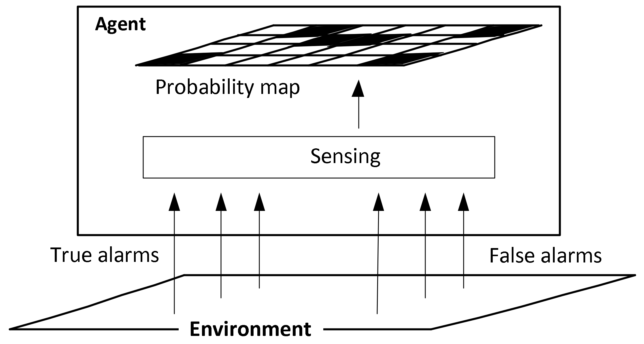
In the framework of the Koopman approach, these probabilities are defined on the basis of Equations (6) and (7) and are represented as follows:
and
The defined process of updating the probabilities is illustrated in
Figure 1.
As illustrated by the figure, the agent receives true and false alarms through its on-board sensors, and based on this information, it updates the targets’ location probabilities with Equations (11) and (12).
In the case of static targets, the location probabilities , , depend only on the agent’s location at time and its movements, while in the case of moving targets, these probabilities are defined both by the targets’ and by the agent’s activities. In the considered problem, it is assumed that the targets act independently on the agent’s motion, while the agent is aware of the process that governs the targets’ motion.
In general, the process of target detection is outlined as follows. At each step, the agent considers the probabilities , , for the targets’ locations and makes a decision regarding its next movement. After moving to the new location (or remaining at its current location), the agent receives signals from the available cells and updates the probabilities following Equations (11) and (12). The obtained updated probabilities are used to continue the process.
The goal is to define the motion of the agent that results in the detection of all targets in minimal time. As indicated above, in detecting the targets, the agent is not required to arrive to their exact locations, but it is required to specify the locations as definitively as possible. Since finding a general definition of the optimal agent’s motion for any nontrivial scenario is computationally intractable, we are interested in a practically computable near-optimal solution.
3. Decision-Making Policy and Deep Q-Learning Solution
Formally, the detection problem of interest is specified as follows. Starting from the initial cell , at time , the agent is located in cell and makes a decision regarding its action that determines to which cell the agent should move from its current location .
3.1. The Agent’s Actions and Decision Making
We assume that the policy for choosing an action does not depend on time and is specified for any by the current agent’s location and probability map . Then, the desired policy should produce actions such that the agent’s trajectory from the cell up to the final cell is as short as possible (in the sense that the termination time is as short as possible), and that by following this trajectory, the agent detects all targets. It is assumed that the number of targets is not available to the agent during detection and is used to indicate the end of the detection process.
With respect to the indicated properties of the desired agent trajectory, a search for the decision-making policy can follow either the maximization of the expected cumulative information gain over the trajectory or the direct optimization of the length of the trajectory in the indicated sense of minimal detection time. The first approach is referred to as the Q-max algorithm, and the second is referred to as the SPL algorithm.
In previous research [
12,
13], a similar search and detection problem is solved heuristically by evaluating the decisions made at each step of the search and detection process. In the first algorithm, the agent follows the maximal Expected Information Gain (
) over the cells that are reachable in a single step from the agent’s current location; in the second algorithm, the agent moves one step toward the maximal expected information gain over all the cells, which is the Center Of View (
) of the domain; and in the third algorithm, the agent moves toward the center of the distribution or the Center Of Gravity (
) with respect to the current probability map.
In this paper, we address a more sophisticated approach that implements deep Q-learning techniques. First, we consider the information-based Q-max algorithm and then the SPL algorithm.
Let us start with the Q-max solution of the considered detection problem. Assume that at each time
the agent is located in cell
and action
is chosen from among the possible movements from cell
, which are to step “forward”, “right-forward”, “right”, “right-backward”, “backward”, “left-backward”, “left”, or “left-forward” or “stay in the current cell”. Symbolically, we write this choice as
Denote by
a probability map that should represent the targets’ locations at time
given that at time
, the agent chooses action
. Then, given action
, the immediate expected informational reward of the agent is defined as
that is, the Kullback–Leibler distance between the map
and the current probability map
. Given a policy
for choosing an action, the expected cumulative discounted reward obtained by an agent that starts in cell
with probability map
and chooses action
is
where as usual, the discount factor is
, and the goal is to find a maximum value
of the expected reward
over all possible policies
that can be applied after action
is chosen at time
.
Since the number of possible policies is infinite, the value of the maximal expected cumulative discounted reward cannot be calculated exactly, and for any realistic scenario, it should be approximated. Below, we follow the deep Q-learning approach and present the Q-max algorithm, which approximates the values of the reward for all possible actions (13) and therefore provides criteria for choosing the actions.
3.2. Dynamic Programming Scheme with Prediction and Target Neural Networks
The learning stage in the suggested Q-max algorithm is based on a neural network with dynamic programming for predicting current rewards. In the simplest configuration, which is still rather effective, the network consists of one input layer, which includes neurons (recall that is the size of the domain); one hidden layer, which also includes . neurons; and an output layer, which includes neurons with respect to the number of possible actions (13).
The inputs of the network are as follows. The first chunk of inputs receives a binary vector that represents the agent location; namely, if the agent is located in cell , then the th input of the network is equal to and the other inputs are equal to . The second chunk of inputs receives the target location probabilities; namely, the th input receives the target location probability , , as it appears in the probability map .
The hidden layer of the network consists of neurons, each of which implements a fully connected linear layer and sigmoid activation function . This activation function was chosen from among several possible activation functions, such as the step function, Softplus function and SiLU function, and it was found that it provides adequate learning in all conducted simulations.
The nine neurons of the output layer correspond to the possible actions. Namely, the first output corresponds to the action , “step forward“; the second output corresponds to the action , “step right-forward”; and so on up to action , which is “stay in the current cell”. The value of the th output is the maximal expected cumulative discounted reward obtained by the agent if it is in cell , , and given the target location probabilities , it chooses action , .
The scheme of the network is shown in
Figure 2.
The training stage of the network implements deep Q-learning techniques, which follow the dynamic programming approach (see, e.g., [
16,
17]). In general, the Bellman equation for calculating the maximal cumulative discounted reward is as follows:
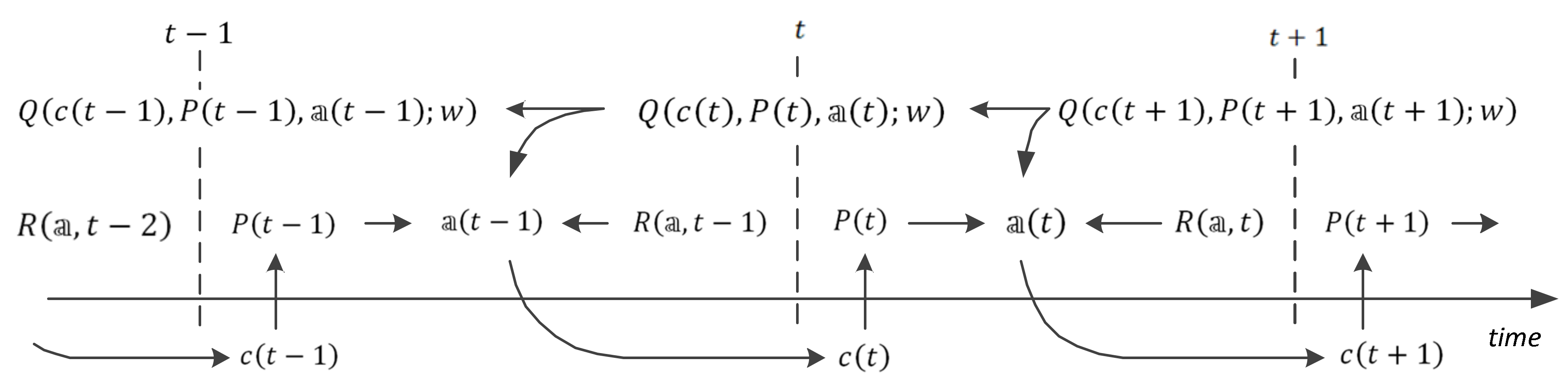
and this equation forms a basis for updating the weights of the links in the network. The data flow specified by this equation is shown in
Figure 3.
Let be a vector of the link weights of the network. In the considered case, there are values of the weights, where is the number of links between the input layers and the hidden layer, is the number of links between the hidden layer and the output layer, is the number of biases in the hidden layer and is the number of biases in the output layer.
In addition, to distinguish these steps and to separate them from the real time, we enumerate the training steps by below and retain the symbol for the real-time moments of the detection process.
Denote by
the maximal cumulative discounted reward calculated at step
by the network with weights
, and denote by
the expected maximal cumulative discounted reward calculated using the vector
of the updated weights following the recurrent Equation (17); that is,
Then, the temporal difference learning error is
In practice, the values and are associated with separate neural networks; the first is called the prediction network, and the second is called the target network.
3.3. Model-Free and Model-Based Learning
The updating of the weights in the prediction network is conducted by following basic backpropagation techniques; namely, the weights for the next step are updated with respect to the temporal difference learning error calculated at the current step . The weights in the target network are updated to the values of the weights after an arbitrary number of iterations. In the simulations presented in subsequent sections, such updating was conducted at every fifth step.
The presented training procedure directly uses the events occurring in the environment and does not require prior knowledge about the targets’ abilities. In other words, by following this procedure, the agent detects the targets in the environment and simultaneously learns the environment and trains the neural network that supports the agent’s decision-making processes. We refer to such a scenario as model-free learning.
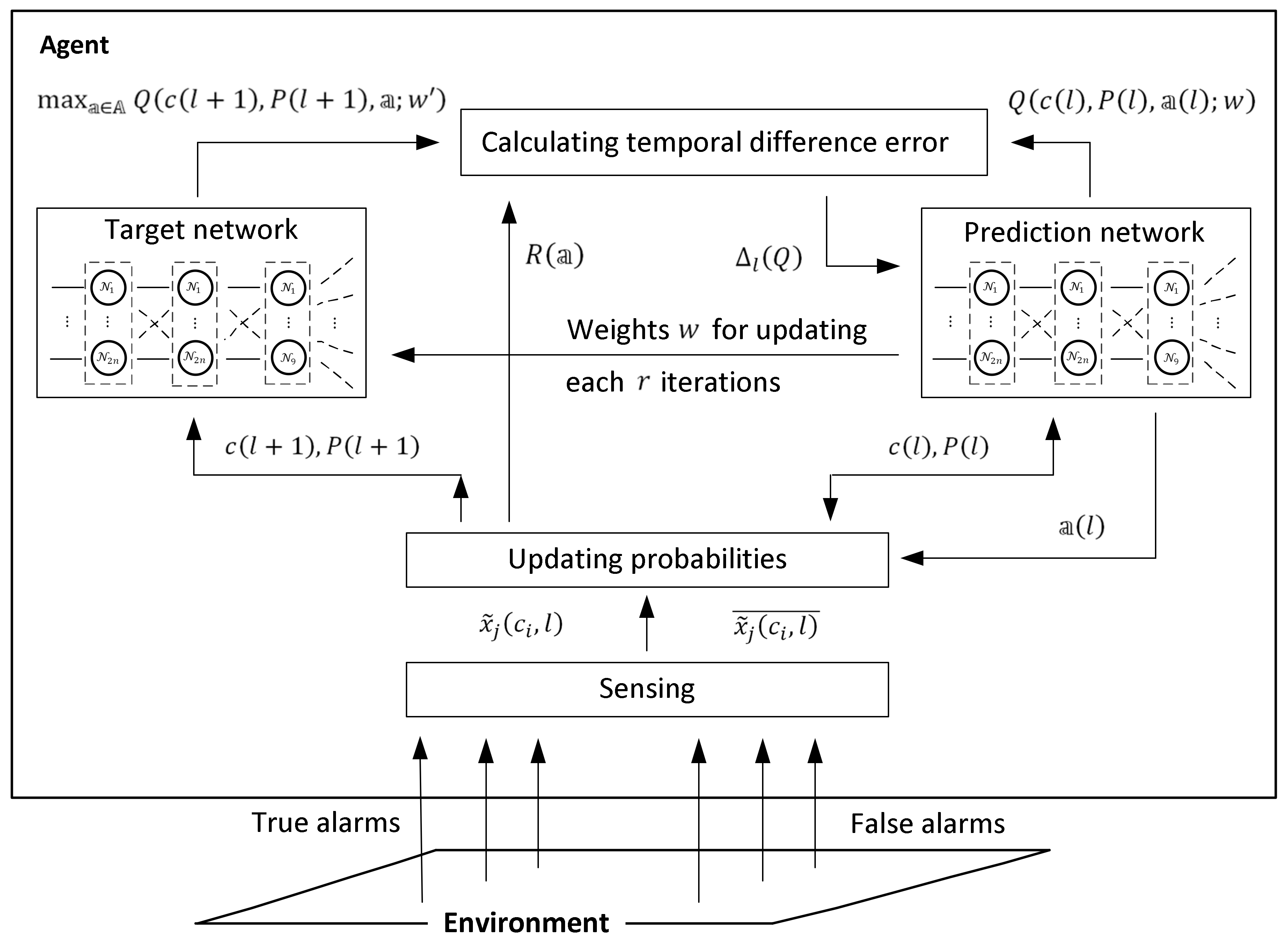
The actions of the presented online model-free learning procedure are illustrated in
Figure 4.
Following the figure, at step , the target location probabilities and , , are updated by Equations (11) and (12) with respect to the events and of receiving and not receiving a signal from cell while the agent is in cell . The updated target location probabilities are used for calculating the value of the immediate reward by Equation (14) and the value by Equation (18) in the target network. In parallel, the value of the prediction network is used for choosing the action and consequently for specifying the expected position of the agent in the environment. After calculating the temporal difference error between the -values in the target and in the prediction network by Equation (19), the weights in the prediction network are updated, and the process continues with step .
Note that in all the above definitions, the cumulative reward does not depend on the previous trajectory of the agent. Hence, the process that governs the agent’s activity is a Markov process with states that include the positions of the agent and the corresponding probability maps. This property allows the use of an additional offline learning procedure based on the knowledge of the targets’ abilities.
Namely, if the abilities of the targets are known and can be represented in the form of transition probability matrices that govern the targets’ motion, the learning process can be conducted offline without checking the events occurring in the environment. In this scenario, at step , instead of the target location probabilities and , , the networks use the probabilities of the expected targets’ locations and at step given the states of the cells at the previous step .
Based on the previous definitions, these probabilities are defined as follows:
and
Since the presented procedure is based on certain knowledge about the targets’ activity, it is called the model-based learning procedure.
The actions of the model-based offline learning procedure are illustrated in
Figure 5.
The model-based learning procedure differs from the model-free learning procedure only in the use of the target location probabilities and the method of updating them. In the model-free procedure, these probabilities are specified based on the events occurring in the environment. In the model-free procedure, they are calculated by following the Markov property of the system without referring to the real events in the environment.
As a result, in the model-free procedure, the learning is slower than in the model-based procedure. However, while in the first case, the agent learns during the detection process and can act without any prior information about the targets’ abilities, in the second case, it starts detection only after offline learning and requires an exact model of the targets’ activity. Thus, the choice of a particular procedure is based on the considered practical task and available information.
3.4. The Choice of the Actions at the Learning Stage
As indicated above, given the agent’s location
and the targets’ probability map
, the neural networks used at the learning stage provide
output
-values that are associated with possible actions
,
, namely,
where
(“step forward”),
(“step right-forward”), and so on up to
(“stay in the current cell”).
The choice among the actions is based on the corresponding -values , , and implements exploration and exploitation techniques. At the initial step , when the agent has no prior learned information about the targets’ locations, action is chosen randomly. Then, after processing the step prescribed by action , the next action is chosen either on the basis of the target location probabilities learned by the neural networks or randomly from among the actions available at this step. The ratio of random choices decreases with the number of steps, and after finalizing the learning processes in the neural networks, the actions are chosen with respect to the -values only.
Formally, this process can be defined using different policies, for example, with a decaying -greedy policy that uses the probability , which decreases with the increase in the number of steps from its maximal value to the minimal value . The agent chooses an action randomly with probability and according to the greedy rule with probability . In this policy, the choice of the action is governed by the probability and does not depend on the -values of the actions.
A more sophisticated policy of intermittence between random and greedy choice is the SoftMax policy. In this policy, the probability
of choosing action
is defined with respect to both the parameter
and the
-values of the actions:
Therefore, if
, then
for
and
for all other actions, and if
, then
, which corresponds to a randomly chosen action. The intermediate values
correspond to the probabilities
and govern the randomness of the action choice. In other words, the value of the parameter
decreases with the increasing number of steps
from its maximal value to zero; thus, for the unlearned networks, the agent chooses actions randomly and then follows the information about the targets’ locations learned by the networks. The first stages with randomly chosen actions are usually interpreted as exploration stages, and the later stages based on the learned information are considered exploitation stages. In the simulations, we considered both policies and finally implemented the SoftMax policy since it provides more correct choices, especially in cases with relatively high
-values associated with different actions.
3.5. Outline of the Q-Max Algorithm
Recall that according to the formulation of the detection problem, the agent acts in the finite two-dimensional domain and moves over this domain with the aim of detecting hidden targets. At time in cell , the agent observes the domain (or, more precisely, screens the domain with the available sensors) and creates the probability map , where is the probability that at time , cell is occupied by a target, . Based on the probability map , the agent chooses an action . By processing the chosen action , the agent moves to the next cell , and this process continues until the targets’ locations are detected. The agent’s goal is to find a policy of choosing the action that provides the fastest possible detection of all the targets with a predefined accuracy.
In contrast to the recently suggested algorithms [
12,
13], which directly implement one-step decision making, the presented novel algorithm includes learning processes and can be used both with model-free learning for direct online detection and with model-based learning for offline policy planning and further online applications of this policy. Since both learning processes follow the same steps (with the only difference being in the source of information regarding the targets’ location probabilities), below, we outline the Q-max algorithm with model-based learning.
The Q-max algorithm with model-based learning includes three stages: in the first stage, the algorithm generates the training data set, which includes reasonable probability maps with possible agent locations; in the second stage, it trains the prediction neural network using the generated data set; and in the third stage, the algorithm solves the detection problem by following the decisions made by the trained prediction neural network. Algorithm 1 outlines the first stage that is generating of the training data set.
| Algorithm 1. Generating the training data set |
| Input: domain , |
| set of possible actions, |
| probability of true alarms (Equation (3)), |
| rate of false alarms and their probability (Equation (4)), |
| sensor sensitivity , |
| range of possible numbers of targets, |
| length of the agent’s trajectory, |
| number of agent trajectories, |
| initial probability map on the domain . |
| Output: data set that is an table of pairs of agent positions and corresponding probability maps . |
| 1. Create the data table. |
| 2. For each agent trajectory do: |
| 3. Choose a number of targets according to a uniform distribution on the interval . |
| 4. Choose the target locations randomly according to the uniform distribution on the domain . |
| 5. Choose the initial agent position randomly according to the uniform distribution on the domain . |
| 6. For do: |
| 7. Save the pair as the th element of the data table. |
| 8. Choose an action randomly according to the uniform distribution on the set . |
| 9. Apply the chosen action and set the next position of the agent. |
| 10. Calculate the next probability map with Equations (20) and (21). |
| 11. End for |
| 12. End for |
| 13. Return the data table. |
The data training data set includes random trajectories of length . Each element of the data set is a pair of an agent position and a probability map.
The reason for generating the data instead of drawing it randomly is that the training data set is used at the learning stage of the prediction network, so it should represent the data in as realistic a form as possible. Since in the generated data set, the agent’s positions are taken from the connected trajectory and the corresponding probability maps are calculated with respect to these positions, possible actions, sensing abilities and environmental conditions, it can be considered a good imitation of real data.
The generated agent positions and corresponding probability maps are used as an input of the prediction neural network in the training stage. The goal of the training is specified by the objective probability map , which defines the target location probabilities that provide sufficient information for the immediate detection of all the targets. In the best case, we have probabilities , and in practical scenarios, it is assumed that either or for certain , .
The training stage of the Q-max algorithm is implemented in the form of Algorithm 2, which is outlined below (the scheme of the learning procedure is shown in
Figure 5).
| Algorithm 2. Training the prediction neural network |
| Network structure: |
| input layer: neurons ( agent positions and target location probabilities, both relative to the size of the domain), |
| hidden layer: neurons, |
| output layer: neurons (in accordance with the number of possible actions). |
| Activation function: |
| sigmoid function . |
| Loss function: |
| mean square error (MSE) function. |
| Input: domain , |
| set of possible actions, |
| probability of true alarms (Equation (3)), |
| rate of false alarms and their probability (Equation (4)), |
| sensor sensitivity , |
| discount factor , |
| objective probability map (obtained by using the value ), |
| number of iterations for updating the weights, |
| initial value (Equation (22)) and its discount factor , |
| learning rate (with respect to the type of optimizer), |
| number of epochs, |
| initial weights of the prediction network and initial weights of the target network, |
| training data set (that is, the table of pairs created by Procedure 1). |
| Output: The trained prediction network. |
| 1. Create the prediction network. |
| 2. Create the target network as a copy of the prediction network. |
| 3. For each epoch do: |
| 4. For each pair from the training data set, do: |
| 5. For each action do: |
| 6. Calculate the value with the prediction network. |
| 7. Calculate the probability (Equation (22)). |
| 8. End for. |
| 9. Choose an action according to the probabilities . |
| 10. Apply the chosen action and set the next position of the agent. |
| 11. Calculate the next probability map with Equations (20) and (21). |
| 12. If or , then |
| 13. Set the immediate reward . |
| 14. Else |
| 15. Calculate the immediate reward with respect to and (Equation (14)). |
| 16. End if. |
| 17. For each action do: |
| 18. If then |
| 19. Set . |
| 20. Else |
| 21. Calculate the value with the target network. |
| 22. End if. |
| 23. End for. |
| 24. Calculate the target value (Equation (17)). |
| 25. Calculate the temporal difference learning error as for the chosen action (Equation (19)) and set for all other actions. |
| 26. Update the weights in the prediction network by backpropagation with respect to the error . |
| 27. Every iterations, set the weights of the target network as . |
| 28. End for. |
The validation of the network was conducted on a validation data set that includes the pairs , which are similar to the pairs appearing in the training data set but were not used in the training procedure; the size of the validation data set is approximately ten percent of the size of the training data set.
After training, the Q-max algorithm can be applied to simulated data or in a real search over a domain. It is clear that the structure of the algorithm mimics the search conducted by rescue and military services: first, the algorithm learns the environment (by itself or at least by using the model) and then continues with the search in the real environment, where the probability map is updated with respect to the received alarms and acquired events (Equations (11) and (12)) and decision-making is conducted using the prediction network.
3.6. The SPL Algorithm
Now let us consider the SPL algorithm. Formally, it follows the same ideas and implements the same approach as the Q-max algorithm, but it differs in the definition of the goal function. In the SPL algorithm, the goal function directly represents the aim of the agent to detect all the targets in a minimal number of steps or to take a minimal number of actions before reaching the termination condition.
In parallel to the reward
defined by Equation (14) for action
conducted at time
, we define the penalty or the price paid by the agent for action
at time
. In the case of the shortest path length, the payoff represents the steps of the agent; that is,
for each time
until termination of the search. Note again that even if the agent chooses to stay at its current position, the payoff is calculated as
.
Then, given a policy
for choosing an action, the expected cumulative payoff of an agent that starts in cell
with probability map
and chooses action
is
and the goal is to find the minimum value
of the expected payoff
over all possible policies
that can be applied after action
is chosen at time
.
Then, the Bellman equation for calculating the defined minimal expected path length is
and the equations that define the training and functionality of the neural networks follow this equation and have the same form as in the Q-max algorithm (with the obvious substitution of maximization by minimization and the use of
).
4. Simulation Results
The suggested algorithm was implemented and tested in several scenarios and its functionality was compared with the functionality of previously developed heuristic algorithms and, in certain simple setups, with the algorithm that provides optimal solution. Numerical simulations include training of neural network, simulation of the detection process by Q-max and SPL algorithms and their comparisons with heuristic and optimal solutions.
Numerical simulations were implemented using basic tools of the Python programming language with the PyTorch machine learning library, and the trials were run on a PC Intel® Core™ i7-10700 CPU with 16 GB RAM. In the simulations, the detection was conducted over a gridded square domain of size cells, and it was assumed that the agent and each target could occupy only one cell. Given this equipment, we measured the run time of the simulations for different datasets, which demonstrated that the suggested algorithms are implementable on usual computers and do not require specific apparats for their functionality.
4.1. Network Training in the Q-Max Algorithm
First, let us consider the simulation of the network training. The purpose of these simulations is to verify the training method and demonstrate a decrease in the temporal difference learning error with an increasing number of learning epochs. Since the network training is the same for both the Q-max and SPL algorithms, we consider the training for the Q-max algorithm.
The training data set was generated using the parameters , , , , , , , and , . The size of the training data set was .
The input parameters in the simulation used the same values of , , , and , and we also specified and with , , , and . The number of epochs in the simulation was .
The initial weights were generated by the corresponding procedures of the PyTorch library. The optimizer used in the simulation was the ADAM optimizer from the PyTorch library.
The average time required for training the prediction neural network was approximately min (on the PC described above), which is a practically reasonable time for an offline procedure. Note that after offline training, online decision-making is conducted directly by immediate choice without additional calculations.
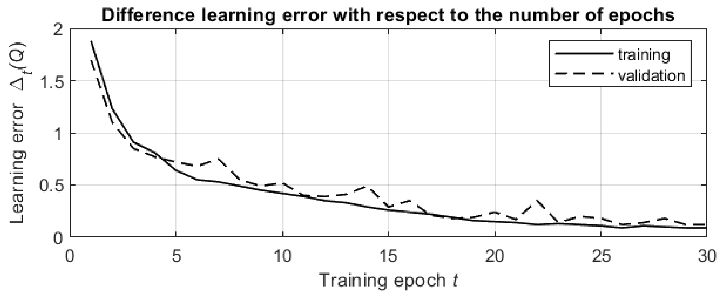
The results of the simulations are shown in
Figure 6. The presented graph was obtained by averaging the temporal difference learning errors over
pairs in the data set.
The temporal difference learning error decreases both in the training stage and in the validation stage of the learning process, and the smoothed graphs for both stages are exponential graphs with similar rates of decrease. This validates the effectiveness of the learning process and shows that progress in the network training leads to better processing of previously unknown data from the validation data set.
4.2. Detection by the Q-Max and SPL Algorithms
In the next simulations, we considered the detection process with the proposed Q-max and SPL algorithms and compared both algorithms with random detection, which provides the lower bound of the cumulative reward (for the Q-max algorithm) and payoff (for the SPL algorithm).
Both algorithms used the same neural network as above, and the random detection process was initialized with the same parameters as above. However, for better comparison, in the simulations of both algorithms and of random detection, we used the same number of targets , which were located at the points and , and the initial position of the agent was . By choosing these positions of the targets and the agent, it is easy to demonstrate (a) the difference between the search processes (in which the agent first moves to the closer target and then to the distant target) and the detection process (in which the agent moves to the point that provides the best observation of both targets) and (b) the motion of the agent over the domain to maximize the immediate reward or minimize the immediate payoff.
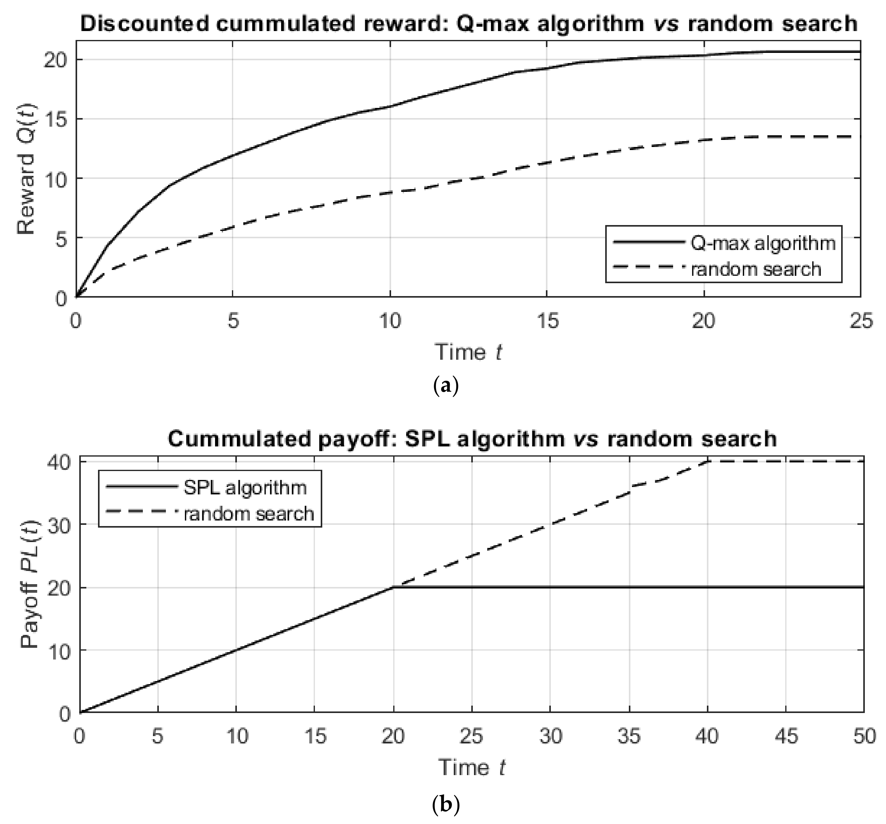
The results of the simulations are shown in
Figure 7.
Figure 7a shows the discounted cumulative reward for the Q-max algorithm in comparison with that of the random detection process, and
Figure 7b shows similar graphs for the SPL algorithm and the random detection process.
The detection by the proposed algorithms is much better than the detection by the random procedure. Namely, the Q-max algorithm results in units of discounted cumulative reward, while the random procedure achieves only units of discounted reward in the same number of steps. In other words, the Q-max algorithm is nearly times more effective than the random procedure. Similarly, while the random procedure requires steps to detect the targets, the SPL algorithm requires only steps, which means that the SPL algorithm is 50% better than the random procedure.
From these comparisons, it follows that the suggested algorithms outperform the random procedure in terms of both the informational reward and the agent’s path length. However, as follows from the next simulations, the numbers of agent actions up to termination in the Q-max and SPL algorithms are statistically equal, allowing either algorithm to be applied with respect to the considered practical task.
4.3. Comparison between the Q-Max and SPL Algorithms and the Eig, Cov and Cog Algorithms
The third set of simulations included comparisons of the suggested Q-max and SPL algorithms with the previously developed heuristic methods [
12,
13], which implement one-step optimization.
The simplest algorithm is based on the expected information gain, which is an immediate expected information reward
as above, here,
stands for the probability map that is expected to represent the targets’ locations at time
given that at time
, the agent chooses action
and
is the current probability map. Then, the next action is chosen as
A more sophisticated algorithm addresses the center of view, which is defined as the cell in which the agent can obtain the maximal expected information gain
where
is a probability map that is expected to represent the targets’ locations at time
when the agent is located in cell
. Then, the next action is chosen as
where
is the distance between the center of view
and cell
, to which the agent moves from its current location
when it executes action
. Note that in contrast to the next location
, which is one of the neighboring cells of the current agent location
, the center of view
is a cell that is chosen from among all
cells of the domain.
Finally, in the third algorithm, the next action is chosen as
where
stands for the “center of gravity”, which is the first moment of the probability map
, and the remaining terms have the same meanings as above.
The Q-max and SPL algorithms used the same neural network as above and were initialized with the same parameters. As above, for all the algorithms, the agent started in the initial position and moved over the domain with the aim of detecting targets.
The first simulations addressed the detection of static targets, which, as above, were located at points and .
The results of the detection by different algorithms are summarized in
Table 1. The results represent the averages over
trials for each algorithm.
The table shows that the proposed Q-max and SPL algorithms outperform previously developed methods in terms of both the number of agent actions and the value of the discounted cumulative information gain.
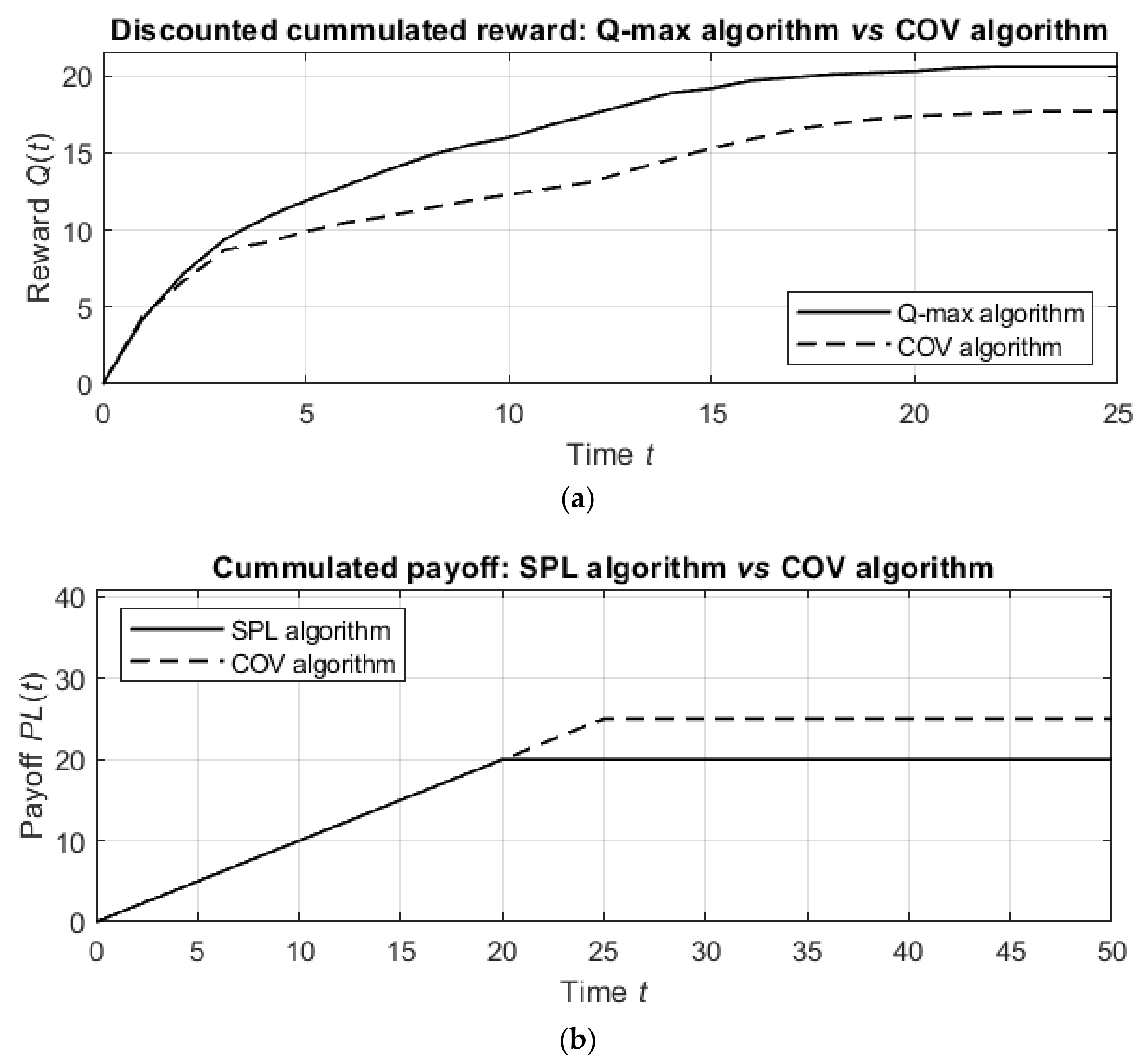
The results of the simulations over time are shown in
Figure 8.
Figure 8a shows the discounted cumulative reward for the Q-max algorithm in comparison with the COV algorithm (the best heuristic algorithm) and the random detection process, and
Figure 8b shows similar graphs for the SPL algorithm compared to the COV algorithm and the random detection process.
The detection by the suggested algorithms is better than the detection by the COV algorithm. Namely, the Q-max algorithm results in units of discounted cumulative reward, while the COV algorithm obtains units of discounted reward in the same number of steps. In other words, the Q-max algorithm is nearly times more effective than the COV algorithm. Similarly, while the COV algorithm requires steps to detect the targets, the SPL algorithm requires only steps, which means that the SPL algorithm is 25% better than the COV algorithm.
The second simulations addressed the detection of moving targets, which started in the initial positions . and . Regarding the targets’ motion, it is assumed that both of them, at each time , can apply one of the possible actions from the set so that the probability of the action is and the probability of each other action is .
The results of detection by different algorithms (averaged over
trials for each algorithm) are summarized in
Table 2.
In the detection of moving targets, the suggested Q-max and SPL algorithms also outperform previously developed methods in terms of both the number of agent actions and the value of the discounted cumulative information gain.
Note that the simulation was conducted for targets with a clear motion pattern, where the probabilities of the targets’ actions represent slow random motion of the targets near their initial locations. Another possible reasonable motion pattern is motion with a strong drift in a certain direction, which results in a similar ratio between the numbers of actions and the discounted cumulative information gains to that presented in
Table 2.
In contrast, if the random motion of the targets is a random walk with equal probabilities for all actions , then the training becomes meaningless since both with and without training, the agent needs to detect randomly moving targets.
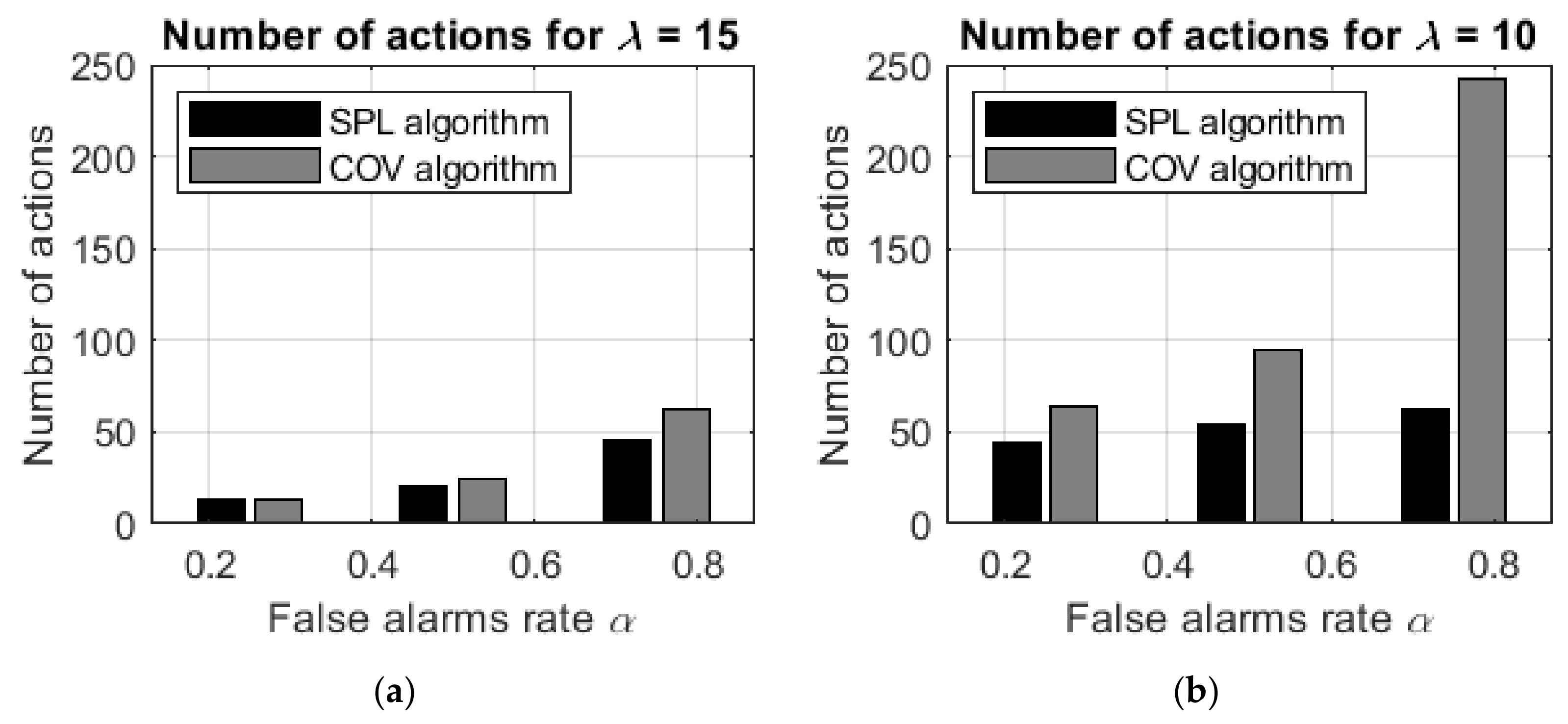
The other results obtained for the Q-max/SPL algorithms also indicated better performance by these algorithms compared with that of the heuristic algorithms. The algorithms were compared with the best heuristic COV algorithm. The results of the trials for different values of the false alarm rate
and of the sensor sensitivity
are summarized in
Table 3.
For all values of the false alarm rate and the sensor sensitivity, the Q-max and SPL algorithms strongly outperform the best heuristic COV algorithm.
To emphasize the difference in the detection time between the suggested SPL and Q-max algorithms and the heuristic COV algorithm, the data shown in the table are depicted in
Figure 9.
As expected, the Q-max and SPL learning algorithms demonstrate better performance than the heuristic COV algorithms without learning, and the difference between the algorithms increases as the false alarm rate increases and the sensor sensitivity decreases. For example, if and , then the improvement in the number of actions is , while if and , then the improvement is significantly stronger at .
In other words, computationally inexpensive heuristic algorithms provide effective results in searches with accurate sensors and a low rate of false alarms. However, in searches with less precise sensors or with a high rate of false-positive errors, the heuristic algorithms are less effective, and the Q-max and SPL learning algorithms should be applied.
4.4. Comparison between the SPL Algorithm and an Algorithm Providing the Optimal Solution
The suggested approach was compared with the known dynamic programming techniques implemented in search algorithms for moving targets [
11,
20]. Since the known algorithms directly address the optimal trajectory of the agent and result in an optimal path, in the simulation, we considered the SPL algorithm, which uses the same criteria as the known algorithms.
The comparisons were conducted as follows. The algorithms were trialed over the same domain with a definite number of cells, and the goal was to reach the maximal probability of detecting the target. When this probability was reached, the trial was terminated, and the number of agent actions was recorded.
Since the known algorithms [
11,
20] implement dynamic programming optimization over possible agent trajectories, their computational complexity is high, and for the considered task, it is
, where
is the number of cells and
is the number of actions.
Therefore, to finish the simulations in reasonable time ( min for each trial), the algorithms were trialed on a very small case with cells. Note that in the original simulations, these algorithms were trialed on smaller cases. If the desired probability of detecting the targets was not reached in min, the algorithms were terminated.
In all trials, the known dynamic programming algorithms planned
agent actions in
min, while the suggested SPL algorithm, in the same time of
min, planned significantly more actions and reached at least the desired probability
of detecting the targets. The results of the comparison between the SPL algorithm and the known dynamic programming algorithms that provide optimal solutions are summarized in
Table 4.
Until termination at
min, the SPL algorithm plans more agent actions and results in higher detection probabilities than the DP algorithm for both values of sensor sensitivity
and for all values of the false alarm rate
. For example, the dependence of the detection probabilities on the run time for sensor sensitivity
and false alarm rate
is depicted in
Figure 10.
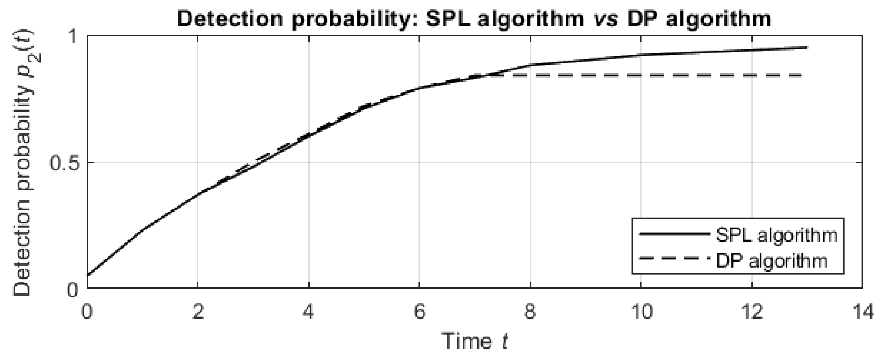
For the first actions, the detection probabilities of both algorithms increase similarly. Then, the DP algorithm does not plan additional actions in min, while the SPL algorithm results in more planned actions, and the detection probabilities for these actions continue increasing until termination after planned actions.
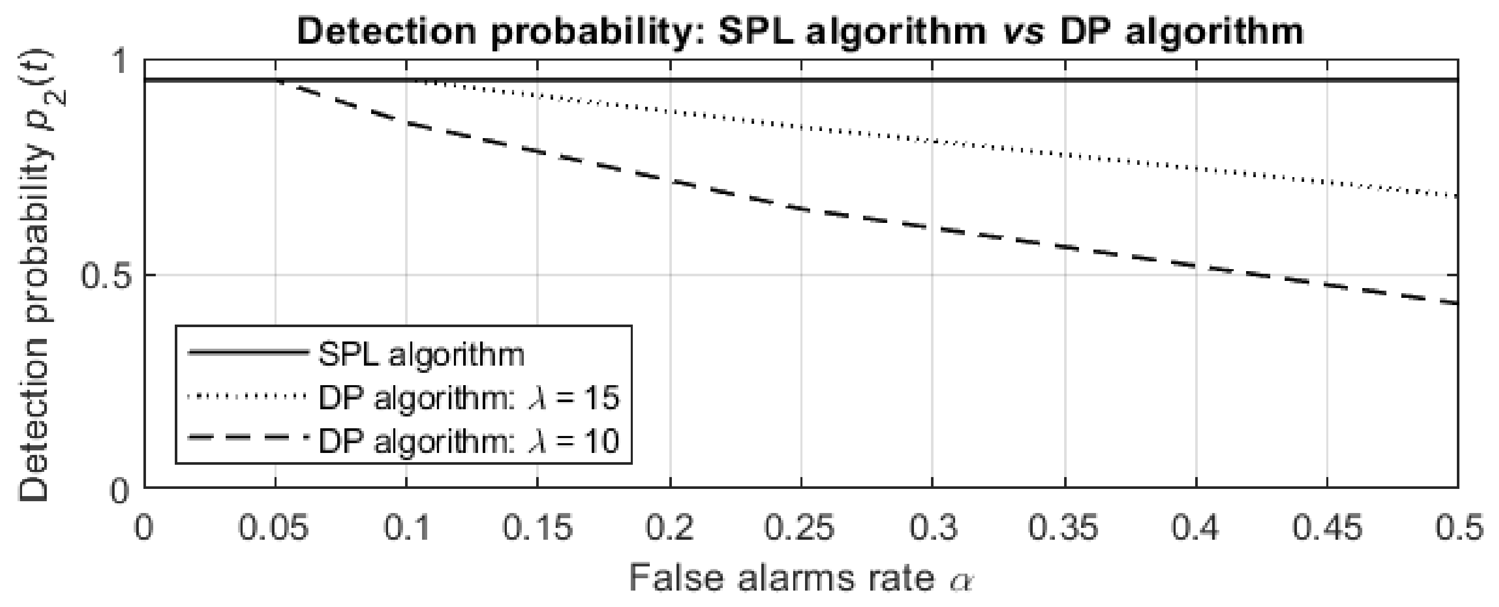
Finally, the dependence of the detection probabilities on the false alarm rate
at termination after
min is depicted in
Figure 11.
For a low false alarm rate , the SPL algorithm results in the same detection probabilities as the optimal DP algorithms, but for a higher false alarm rate , the detection probabilities obtained by the DP algorithms significantly decrease (to and for and , respectively), while the probability obtained by the SPL algorithm is for any false alarm rate and both sensor sensitivities.
4.5. Run Times and Mean Squared Error for Different Sizes of Data Sets
Finally, we considered the dependence of the run time and mean squared error on the size of the data set. The results of these simulations are summarized in
Table 5.
While the size of the domain and the number of links in the network exponentially increase, the mean squared error increases very slowly and remains small. In addition, it is seen that with an exponentially increasing domain size, the run time increases linearly, and the computations require a reasonable time even on the previously described PC. However, for realistic engineering and industrial problems with larger domains, it is reasonable to use computation systems with greater GPU power.
6. Conclusions
This paper considered the detection problem for multiple static and moving targets hidden in a domain, directly extending the classical Koopman search problem. Following previously developed methods, we addressed detection with both false-positive and false-negative detection errors.
In the exploration stage, the suggested algorithm implements the deep Q-learning approach and applies neural network techniques for learning the probabilities of the targets’ locations and their motion patterns; then, in the exploitation stage, it chooses actions based on the decisions made by the trained neural network.
The research suggested two possible procedures. In the first, called the model-free procedure, the agent detects the targets in the environment and simultaneously, online, learns the environment and trains a neural network that supports the agent’s decision-making processes. In the second procedure, called the model-based procedure, the agent begins detection only after offline learning and requires an exact model of the targets’ activity.
The results obtained by maximizing the discounted cumulative expected information gain and by minimizing the expected length of the agent’s path demonstrate that the suggested algorithm outperforms previously developed information-based procedures and provides a nearly optimal solution even in cases in which the existing techniques require an unreasonable computation time.
The proposed algorithms were implemented in the Python programming language and can be used both for further development of the methods of probabilistic search and detection and for practical applications in the appropriate fields.


