
Goal or Miss? A Bernoulli Distribution for In-Game Outcome Prediction in Soccer

Abstract
:
1. Introduction
2. Methods
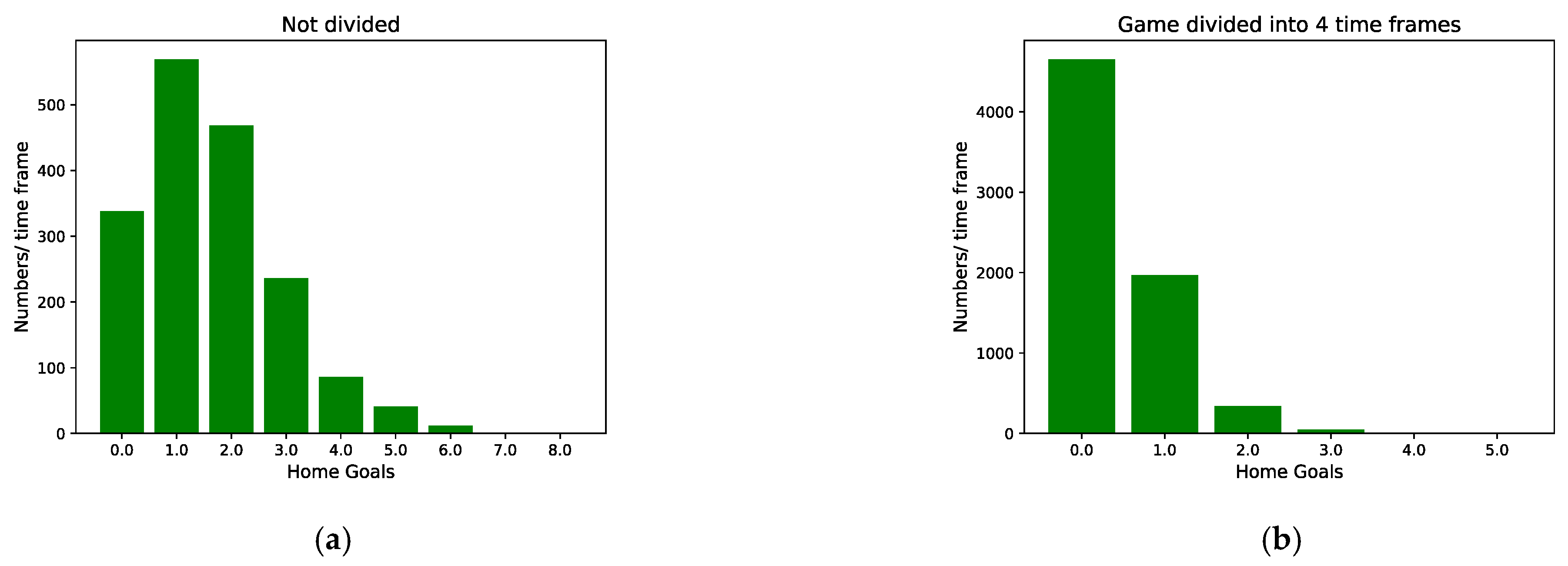
2.1. Modeling
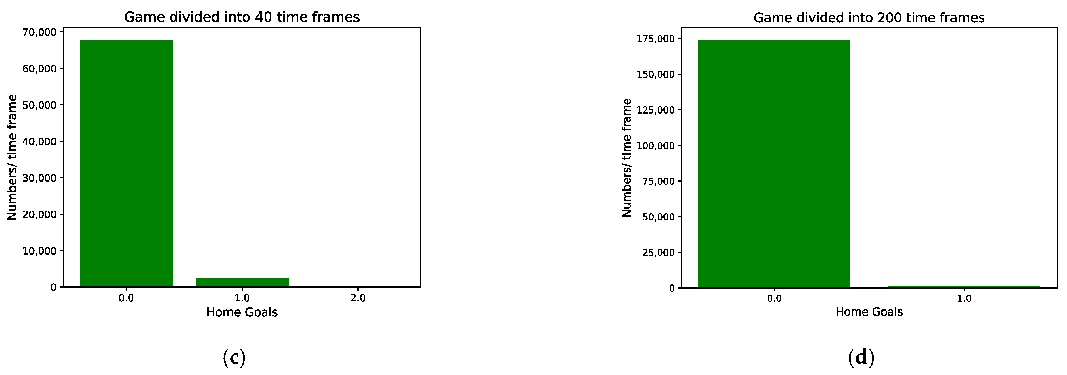
2.2. Flow Framework
2.3. Feature Engineering
3. Results
3.1. Prediction Models
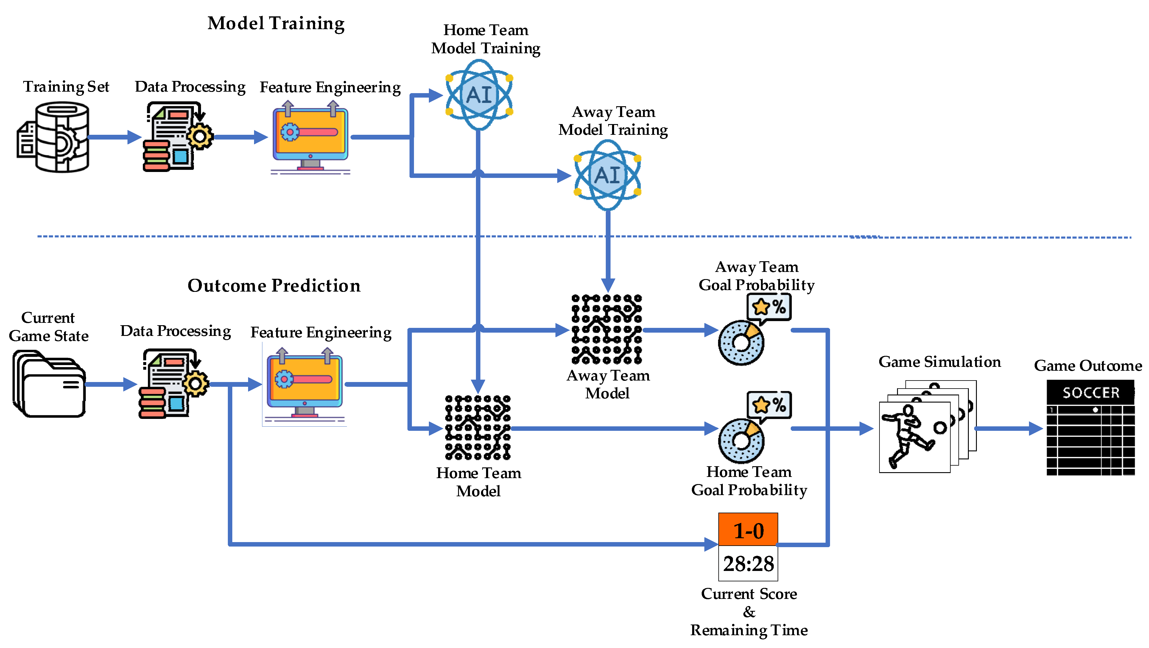
3.2. Method Evaluation
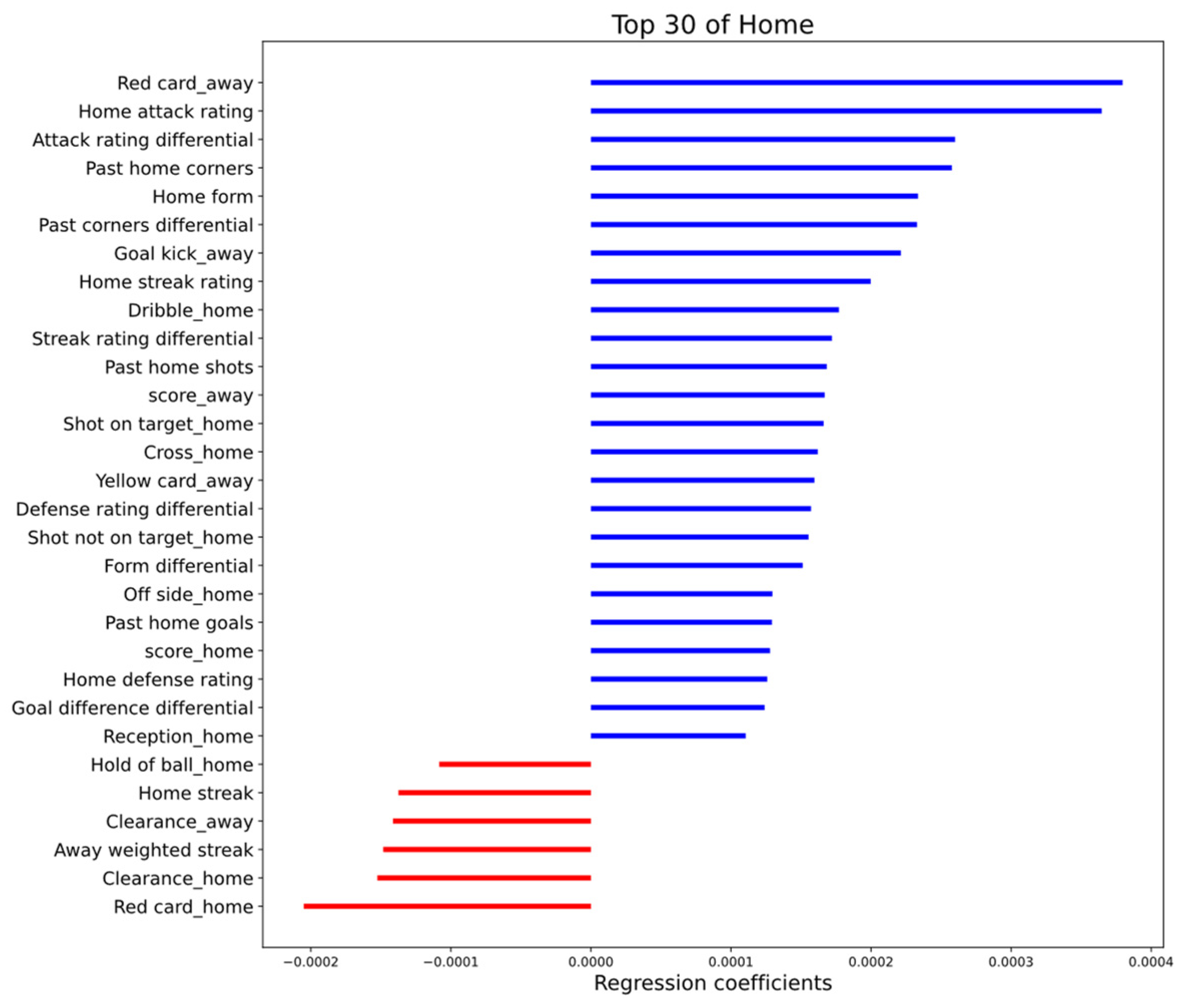
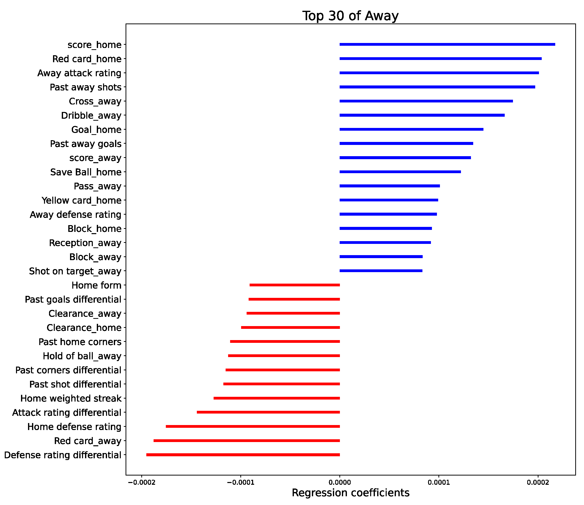
3.3. Feature Importance
4. Discussion and Conclusions
Author Contributions
Funding
Data Availability Statement
Conflicts of Interest
References
- Sports Industry Statistic and Market Size Overview, Business and Industry Statistics. Available online: https://www.plunkettresearch.com/statistics/Industry-Statistics-Sports-Industry-Statistic-and-Market-Size-Overview (accessed on 25 May 2022).
- Liu, L.; Hodgins, J. Learning basketball dribbling skills using trajectory optimization and deep reinforcement learning. ACM Trans. Graph. (TOG) 2018, 37, 1–14. [Google Scholar] [CrossRef]
- King, B.E.; Rice, J. Predicting Attendance at Major League Soccer Matches: A Comparison of Four Techniques. J. Comput. Sci. Inf. Technol. 2018, 6, 15–22. [Google Scholar] [CrossRef]
- Strnad, D.; Nerat, A.; Kohek, Š. Neural network models for group behavior prediction: A case of soccer match attendance. Neural Comput. Appl. 2017, 28, 287–300. [Google Scholar] [CrossRef]
- Yamashita, G.H.; Fogliatto, F.S.; Anzanello, M.J.; Tortorella, G.L. Customized prediction of attendance to soccer matches based on symbolic regression and genetic programming. Expert Syst. Appl. 2022, 187, 115912. [Google Scholar] [CrossRef]
- Lysens, R.; Steverlynck, A.; Auweele, Y.V.D.; Lefevre, J.; Renson, L.; Claessens, A.; Ostyn, M. The Predictability of Sports Injuries. Sports Med. 1984, 1, 6–10. [Google Scholar] [CrossRef]
- Luu, B.C.; Wright, A.L.; Haeberle, H.S.; Karnuta, J.M.; Schickendantz, M.S.; Makhni, E.C.; Nwachukwu, B.U.; Williams, I.R.J.; Ramkumar, P.N. Machine Learning Outperforms Logistic Regression Analysis to Predict Next-Season NHL Player Injury: An Analysis of 2322 Players From 2007 to 2017. Orthop. J. Sports Med. 2020, 8, 2325967120953404. [Google Scholar] [CrossRef]
- Ahmad, C.S.; Dick, R.W.; Snell, E.; Kenney, N.D.; Curriero, F.C.; Pollack, K.; Albright, J.P.; Mandelbaum, B.R. Major and minor League baseball hamstring injuries: Epidemiologic findings from the major league baseball injury surveillance system. Am. J. Sports Med. 2014, 42, 1464–1470. [Google Scholar] [CrossRef]
- Sarlis, V.; Chatziilias, V.; Tjortjis, C.; Mandalidis, D. A Data Science approach analysing the Impact of Injuries on Basketball Player and Team Performance. Inf. Syst. 2021, 99, 101750. [Google Scholar] [CrossRef]
- Dijkhuis, T.; Kempe, M.; Lemmink, K. Early Prediction of Physical Performance in Elite Soccer Matches—A Machine Learning Approach to Support Substitutions. Entropy 2021, 23, 952. [Google Scholar] [CrossRef]
- Fuller, C.W. Modeling the impact of players’ workload on the injury-burden of English Premier League football clubs. Scand. J. Med. Sci. Sports 2018, 28, 1715–1721. [Google Scholar] [CrossRef]
- Decroos, T.; Bransen, L.; Van Haaren, J.; Davis, J. Actions Speak Louder than Goals: Valuing Player Actions in Soccer. In Proceedings of the Kdd’19: Proceedings of the 25th Acm Sigkdd International Conferencce on Knowledge Discovery and Data Mining, Anchorage, AK, USA, 4–8 August 2019. [Google Scholar]
- Bialkowski, A.; Lucey, P.; Carr, P.; Yue, Y.; Sridharan, S.; Matthews, I. Large-scale analysis of soccer matches using spatiotemporal tracking data. In Proceedings of the 2014 IEEE International Conference on Data Mining, Shenzhen, China, 14–17 December 2014. [Google Scholar]
- Bialkowski, A.; Lucey, P.; Carr, P.; Matthews, I.; Sridharan, S.; Fookes, C. Discovering Team Structures in Soccer from Spatiotemporal Data. IEEE Trans. Knowl. Data Eng. 2016, 28, 2596–2605. [Google Scholar] [CrossRef] [Green Version]
- Wu, Y.; Xie, X.; Wang, J.; Deng, D.; Liang, H.; Zhang, H.; Cheng, S.; Chen, W. ForVizor: Visualizing Spatio-Temporal Team Formations in Soccer. IEEE Trans. Vis. Comput. Graph. 2018, 25, 65–75. [Google Scholar] [CrossRef]
- Thabtah, F.; Zhang, L.; Abdelhamid, N. NBA Game Result Prediction Using Feature Analysis and Machine Learning. Ann. Data Sci. 2019, 6, 103–116. [Google Scholar] [CrossRef]
- Chen, W.-J.; Jhou, M.-J.; Lee, T.-S.; Lu, C.-J. Hybrid Basketball Game Outcome Prediction Model by Integrating Data Mining Methods for the National Basketball Association. Entropy 2021, 23, 477. [Google Scholar] [CrossRef]
- Chen, T.; Guestrin, C. Xgboost: A scalable tree boosting system. In Proceedings of the 22nd Acm Sigkdd International Conference on Knowledge Discovery and Data Mining, San Francisco, CA, USA, 13–17 August 2016. [Google Scholar]
- Landers, J.R.; Duperrouzel, B. Machine Learning Approaches to Competing in Fantasy Leagues for the NFL. IEEE Trans. Games 2018, 11, 159–172. [Google Scholar] [CrossRef]
- Baboota, R.; Kaur, H. Predictive analysis and modelling football results using machine learning approach for English Premier League. Int. J. Forecast. 2019, 35, 741–755. [Google Scholar] [CrossRef]
- Robberechts, P.; Van Haaren, J.; Davis, J. A Bayesian Approach to In-Game Win Probability in Soccer. In Proceedings of the 27th ACM SIGKDD Conference on Knowledge Discovery & Data Mining, Online, Singapore, 14–18 August 2021. [Google Scholar]
- Stern, H.S. A Brownian motion model for the progress of sports scores. J. Am. Stat. Assoc. 1994, 89, 1128–1134. [Google Scholar] [CrossRef]
- Kayhan, V.O.; Watkins, A. A Data Snapshot Approach for Making Real-Time Predictions in Basketball. Big Data 2018, 6, 96–112. [Google Scholar] [CrossRef] [PubMed] [Green Version]
- Lock, D.; Nettleton, D. Using random forests to estimate win probability before each play of an NFL game. J. Quant. Anal. Sports 2014, 10, 197–205. [Google Scholar] [CrossRef] [Green Version]
- Pelechrinis, K. iWinRNFL: A Simple, Interpretable & Well-Calibrated In-Game Win Probability Model for NFL. arXiv 2017, arXiv:1704.00197. [Google Scholar]
- Zou, Q.; Song, K.; Shi, J. A Bayesian In-Play Prediction Model for Association Football Outcomes. Appl. Sci. 2020, 10, 2904. [Google Scholar] [CrossRef] [Green Version]
- Klemp, M.; Wunderlich, F.; Memmert, D. In-play forecasting in football using event and positional data. Sci. Rep. 2021, 11, 24139. [Google Scholar] [CrossRef]
- Kucukelbir, A.; Tran, D.; Ranganath, R.; Gelman, A.; Blei, D.M. Automatic differentiation variational inference. J. Mach. Learn. Res. 2017, 18, 1–45. [Google Scholar]
- Singh, K. Introducing Expected Threat (xT). 2019. Available online: https://karun.in/blog/expected-threat.html (accessed on 25 May 2022).
- Karlis, D.; Ntzoufras, I. On modelling soccer data. Student 2000, 3, 229–244. [Google Scholar]
- Dixon, M.J.; Coles, S.G. Modelling Association Football Scores and Inefficiencies in the Football Betting Market. J. R. Stat. Soc. Ser. C (Appl. Stat.) 1997, 46, 265–280. [Google Scholar] [CrossRef]
- Lee, A.J. Modeling scores in the Premier League: Is Manchester United really the best? Chance 1997, 10, 15–19. [Google Scholar] [CrossRef]
- Karlis, D.; Ntzoufras, I. Analysis of sports data by using bivariate Poisson models. J. R. Stat. Soc. Ser. D (Stat.) 2003, 52, 381–393. [Google Scholar] [CrossRef]
- Pedregosa, F.; Varoquaux, G.; Gramfort, A.; Michel, V.; Thirion, B.; Grisel, O.; Blondel, M.; Prettenhofer, P.; Weiss, R.; Dubourg, V.; et al. Scikit-learn: Machine learning in Python. J. Mach. Learn. Res. 2011, 12, 2825–2830. [Google Scholar]
- Syarif, I.; Prugel-Bennett, A.; Wills, G. SVM parameter optimization using grid search and genetic algorithm to improve classification performance. Telkomnika 2016, 14, 1502. [Google Scholar] [CrossRef]
- Hoerl, A.E.; Kennard, R.W. Ridge regression: Biased estimation for nonorthogonal problems. Technometrics 1970, 12, 55–67. [Google Scholar] [CrossRef]
- Tipping, M.E. Sparse Bayesian learning and the relevance vector machine. J. Mach. Learn. Res. 2001, 1, 211–244. [Google Scholar]
- Breiman, L. Random forests. Mach. Learn. 2001, 45, 5–32. [Google Scholar] [CrossRef] [Green Version]
- Chai, T.; Draxler, R.R. Root mean square error (RMSE) or mean absolute error (MAE)?–Arguments against avoiding RMSE in the literature. Geosci. Model Dev. 2014, 7, 1247–1250. [Google Scholar] [CrossRef] [Green Version]
- Cameron, A.C.; Windmeijer, F.A. R-squared measures for count data regression models with applications to health-care utilization. J. Bus. Econ. Stat. 1996, 14, 209–220. [Google Scholar]
- Epstein, E.S. A scoring system for probability forecasts of ranked categories. J. Appl. Meteorol. 1969, 8, 985–987. [Google Scholar] [CrossRef] [Green Version]
- Constantinou, A.C. Dolores: A model that predicts football match outcomes from all over the world. Mach. Learn. 2019, 108, 49–75. [Google Scholar] [CrossRef] [Green Version]
- Constantinou, A.C.; Fenton, N.E. Solving the problem of inadequate scoring rules for assessing probabilistic football forecast models. J. Quant. Anal. Sports 2012, 8. [Google Scholar] [CrossRef]
- Dietterich, T.G. Approximate statistical tests for comparing supervised classification learning algorithms. Neural Comput. 1998, 10, 1895–1923. [Google Scholar] [CrossRef] [Green Version]
- Niculescu-Mizil, A.; Caruana, R. Predicting good probabilities with supervised learning. In Proceedings of the 22nd International Conference on Machine Learning, New York, NY, USA, 7–11 August 2005. [Google Scholar]
- Guo, C.; Pleiss, G.; Sun, Y.; Weinberger, K.Q. On calibration of modern neural networks. In Proceedings of the International Conference on Machine Learning, PMLR, Sydney, Australia, 6–11 August 2017. [Google Scholar]
- Vaswani, A.; Shazeer, N.; Parmar, N.; Uszkoreit, J.; Jones, L.; Gomez, A.N.; Kaiser, Ł.; Polosukhin, I. Attention is all you need. In Advances in Neural Information Processing Systems; Neural Information Processing Systems Foundation, Inc.: La Jolla, CA, USA, 2017; Volume 30. [Google Scholar]

| Home Features | Away Features | Differential Features |
|---|---|---|
| Home form | Away form | Form differential |
| Home streak | Away streak | Streak differential |
| Past 10 home shots | Past 10 away shots | Past 10 shots differential |
| Past 10 home goals | Past 10 away goals | Past 10 goals differential |
| Past 10 home corners | Past 10 away corners | Past 10 corners differential |
| Home attack rating | Away attack rating | Attack rating differential |
| Home defense rating | Away defense rating | Defense rating differentia |
| Home streak rating | Away streak rating | Streak rating differential |
| Home goal difference | Away goal difference | Goal difference differential |
| Home weighted streak | Away weighted streak | Weighted streak differential |
| Event Type | Description |
|---|---|
| Block | A player blocks a shot on target from an opposing player |
| Save the ball | A goalkeeper preventing the ball from entering the goal |
| Chance | A situation where a player should be expected to score |
| Clearance | A player kicks the ball away from his own goal |
| Cross | A ball played in from wide areas into the box |
| Dribble | A player attempts to beat an opponent when he is in possession |
| Drop of ball | A goalkeeper tries to catch the ball, but drops it from his grasp |
| Penalty | Foul resulting in a free-kick, penalty, and player out |
| Hold of ball | A goalkeeper holds the ball in his hands |
| Own goal | A player kicks a ball into his own net |
| Pass | Any intentional played ball from one player to another |
| Reception | Receive the ball from another player |
| Corner | A kick is taken from the corner of the field |
| Shot not on target | Shot off the net |
| Shot on target | Shot into the net, no matter score or not |
| Tackle | A player takes the ball away from the player in possession. |
| Free-kick | Direct free-kick and indirect free-kick |
| Goal kick | The goalkeeper restarts the game and kicks the ball |
| Goal | Goal and score |
| Offside | A player who is in an offside position when the pass was made |
| Yellow card | A player is shown a yellow card |
| Red card | A player is shown a straight red card |
| R2 | MAE | RMSE | |
|---|---|---|---|
| Ridge Linear Regression | 3.695 × 10⁻² | 1.619 × 10⁻⁴ | 1.272 × 10⁻² |
| Bayesian Ridge Regression | 3.393 × 10⁻² | 1.623 × 10⁻⁴ | 1.274 × 10⁻² |
| RF | 2.443 × 10⁻² | 1.640 × 10⁻⁴ | 1.280 × 10⁻² |
| XGB | 3.033 × 10⁻² | 1.630 × 10⁻⁴ | 1.276 × 10⁻² |
| R2 | MAE | RMSE | |
|---|---|---|---|
| Ridge Linear Regression | 1.007 × 10⁻² | 1.508 × 10⁻⁴ | 1.228 × 10⁻² |
| Bayesian Ridge Regression | 0.995 × 10⁻² | 1.508 × 10⁻⁴ | 1.228 × 10⁻² |
| RF | 0.135 × 10⁻² | 1.521 × 10⁻⁴ | 1.233 × 10⁻² |
| XGB | 0.560 × 10⁻² | 1.515 × 10⁻⁴ | 1.231 × 10⁻² |
| First Half | Second Half | Final 25% | Final 10% | Overall | |
|---|---|---|---|---|---|
| MC | 0.1811 | 0.1099 | 0.0904 | 0.0758 | 0.1455 |
| PD | 0.1778 (−1.82%) | 0.0913 (−16.9%) | 0.0609 (−32.6%) | 0.0318 (−58.0%) | 0.1346 (−7.49%) |
| IGSOP | 0.1755 (−3.09%) | 0.0892 (−18.8%) | 0.0570 (−36.9%) | 0.0270 (−64.4%) | 0.1323 (−9.07%) |
| t-Statistic | p-Value | |
|---|---|---|
| IGSOP/MC | −4.512 | 0.006 < 0.05 |
| PD/MC | −3.270 | 0.022 < 0.05 |
| IGSOP/PD | −1.689 | 0.152 > 0.05 |
Publisher’s Note: MDPI stays neutral with regard to jurisdictional claims in published maps and institutional affiliations. |
© 2022 by the authors. Licensee MDPI, Basel, Switzerland. This article is an open access article distributed under the terms and conditions of the Creative Commons Attribution (CC BY) license (https://creativecommons.org/licenses/by/4.0/).
Share and Cite
Yao, W.; Wang, Y.; Zhu, M.; Cao, Y.; Zeng, D. Goal or Miss? A Bernoulli Distribution for In-Game Outcome Prediction in Soccer. Entropy 2022, 24, 971. https://doi.org/10.3390/e24070971
Yao W, Wang Y, Zhu M, Cao Y, Zeng D. Goal or Miss? A Bernoulli Distribution for In-Game Outcome Prediction in Soccer. Entropy. 2022; 24(7):971. https://doi.org/10.3390/e24070971
Chicago/Turabian StyleYao, Wendi, Yifan Wang, Mengyao Zhu, Yixin Cao, and Dan Zeng. 2022. "Goal or Miss? A Bernoulli Distribution for In-Game Outcome Prediction in Soccer" Entropy 24, no. 7: 971. https://doi.org/10.3390/e24070971
APA StyleYao, W., Wang, Y., Zhu, M., Cao, Y., & Zeng, D. (2022). Goal or Miss? A Bernoulli Distribution for In-Game Outcome Prediction in Soccer. Entropy, 24(7), 971. https://doi.org/10.3390/e24070971