4.1. Data Description Analysis
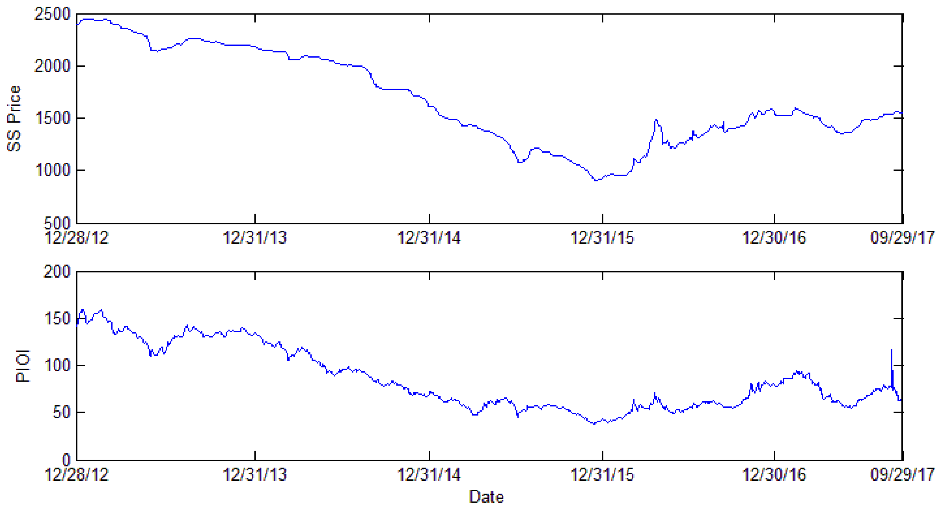
Figure 1 shows the variation trend of steel scrap price and the Platts iron ore index.
Figure 1 shows that the tendency is quite similar: From 12 December 2012 (2394.69) to 8 June 2013 (2138.75), the steel scrap price was always going down. After a two-month increase from 8 June 2013 (2138.75) to 22 August 2013 (2262.34), the steel scrap price fluctuated slowly until 17th December 2015 (905.63). In the former part of 2016, there was a sharp growth in steel scrap prices, which reached 1487.5 on 25 April 2015. Then, the price decreased and fluctuated at a relatively stable level. In 2017, the steel scrap price decreased to 1353.13 on 27 May 2017, and then rose to 1551.88 on 19 September 2017, the end of the sample period.
The steel scrap price is closely related to environmental policy and whole steel market performance. In the former part of 2013, the steel scrap price experienced a downturn until 8 June (2138.75). Then, the price climbed to 2262.34 on 22 August 2013. Then, the steel scrap price underwent a two-year depression until 17 December 2015, and the steel scrap price reached 905.63 yuan per ton. However, in the following 4 months, the steel scrap price increased to 1487.5 on 25 April 2016. Then, the price suddenly dropped to 1217.5 on 3 June 2016. Then, the steel scrap price rose along with fluctuations. In 2017, the scrap steel price experienced a decreasing and increasing period.
The Platts iron ore index uses the spot price, which is based on 62% Fe iron ore CFR (cost and freight) prices of the Qingdao steel market, a major China steel market. The spot price can better reflect the fluctuation tendency of the iron ore index and is widely used by steel market individuals, such as steel-making companies, traders, and mining companies. In June 2013, the PIOI index reached its lowest point (110.75) in 2013 and then climbed to 142.5 on 14 August. Subsequently, the PIOI index fluctuated to decrease until it reached the lowest point (38.5) in the sample period on 15 December 2015. In 2016, iron ore trading began to recover, and during the whole year, the PIOI index increased slowly except for the period from 21 April (70.5) to 9 May (54.85) and the period from 23 August (62.5) to 20 September (55.1). In 2017, the rising tendency continued until 21 February (95.05). Then, there is a sharp decline from 21 February (95.05) to 13 June (54). Then, the index increased, and on 7 September, there was a dramatic increase. The index was up to 116. Then, the PIOI fluctuated and fell.
In the former part of 2013, the steel material market fluctuated in a normal economic cycle. After the Chinese Spring Festival, the launched “Country of Five” policy reduced the expectation of the real estate market. Moreover, excessive inventory in iron and steel enterprises also worsened the situation. The upstream steel material market, therefore, declined. In July 2013, the steel material market began to recover, and expectations decreased a few months ago, thus causing the steel material supply to be tight. Macroeconomic statistical data issuance at this time also strengthened steel companies’ confidence in increasing production. From August 2013, however, the major international iron ore companies greatly improved their production capacity, while in China, this major iron ore consumer greatly reduced its steel production capacity because the environmental regulation in Hebei and Jiangsu Provinces curtails the steel capacity. During 2014, steel material demands in Asia, especially China, decreased. In 2015, a new environmental protection law was enforced. Ambiguous real estate prospects and the enactment of environmental protection policy reduced the capacity of steel enterprises and market expectations, which showed a lack confidence in 2014 and 2015, caused steel material to weaken in demand, and the market went into a downturn for these two years.
In 2016, as steel industry regulations such as cutting-capacity policies came into effect, steel enterprises started making profits again. Downstream demand upsurges led to steel product price increases, as did steel materials. However, in late April, a sudden steel price reduction led the amount of steel material market trading to shrink. Later, continuing market recovery and enterprise production activity caused a rebound in the market. In 2017, the downstream, construction-related demand driving force was limited. Other transportation infrastructure establishment stirs up the market expectation, but it takes time to test the actual economic effect. Upstream, China severely strikes substandard steel and medium frequency furnace steelmaking, considerable steel scrap flows into the market, and the steel scrap price greatly decreases. Like the price of steel scrap substitutes, the iron ore price also decreases. As backward capacity continues to be eliminated, the steel material market begins to run within a reasonable range. Concerning market supply and demand, the steel market is still recovering.
However, does the steel material price lead to the steel product price, or does the steel product price lead to the steel material price on earth?
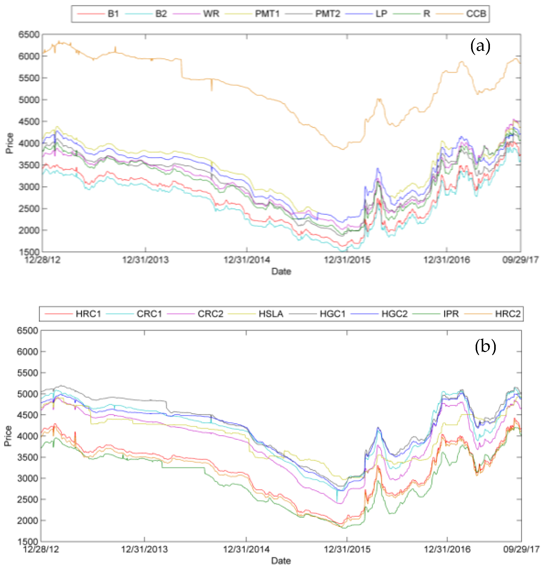
In the actual steel market, as the most vital downstream phase, steel industry development influences the steel material price. The steel products connect the upstream material and downstream demand. Sixteen midstream and downstream steel product prices are presented in
Figure 2.
Figure 2a,b show different steel product price fluctuation trends. Overall, the price variation represents a similar trend to steel material variation. Namely, from 2013, steel demand decreases. Environment regulation activity curtails industry production, and cutting-capacity activity eliminates backward steel capacity. The whole industry goes into a downturn. Until 2016, when the industry regulation in the past few years came into effect, the external economic environment also improved to a stable level, and the steel product price started to rebound. Prior to 2016, infrastructure construction was put into practice and reducing steel inventories pushed steel prices to grow. Steel product price growth gave the market individual confidence about market recovery, and this confidence accelerated the price surge again. However, these short-term soars lacked stable market fundamentals, and product prices tumbled considerably to a reasonable range. Then, the steel product price gradually increased as domestic and foreign demand recovered. In 2017, the real estate market was ambiguous, and it decreased the downstream demand. Additionally, this year, China struggled to eliminate substandard steel. Regulation improves the product quality and increases the enterprise profits. Therefore, there was a down and uptrend in 2017.
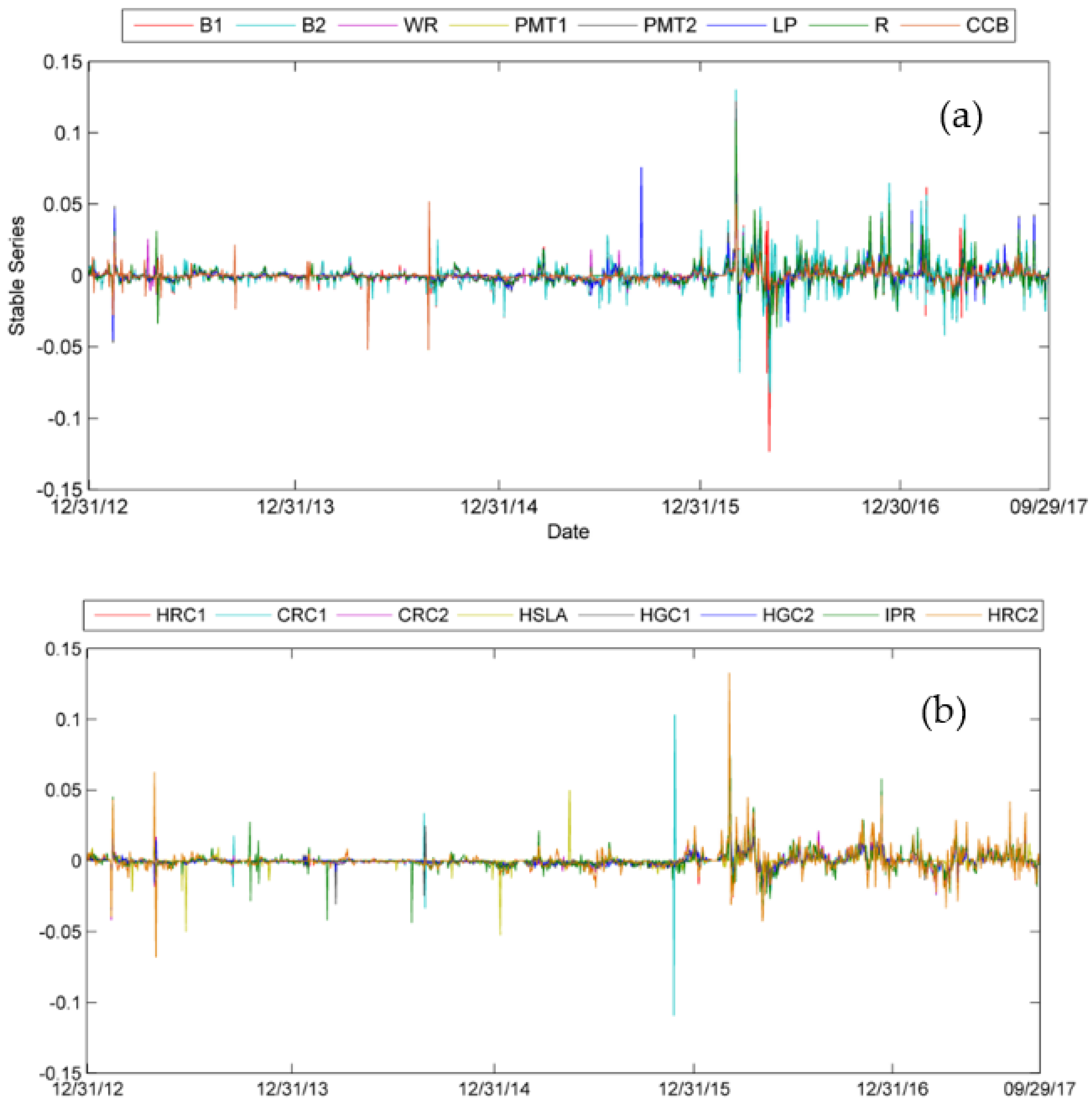
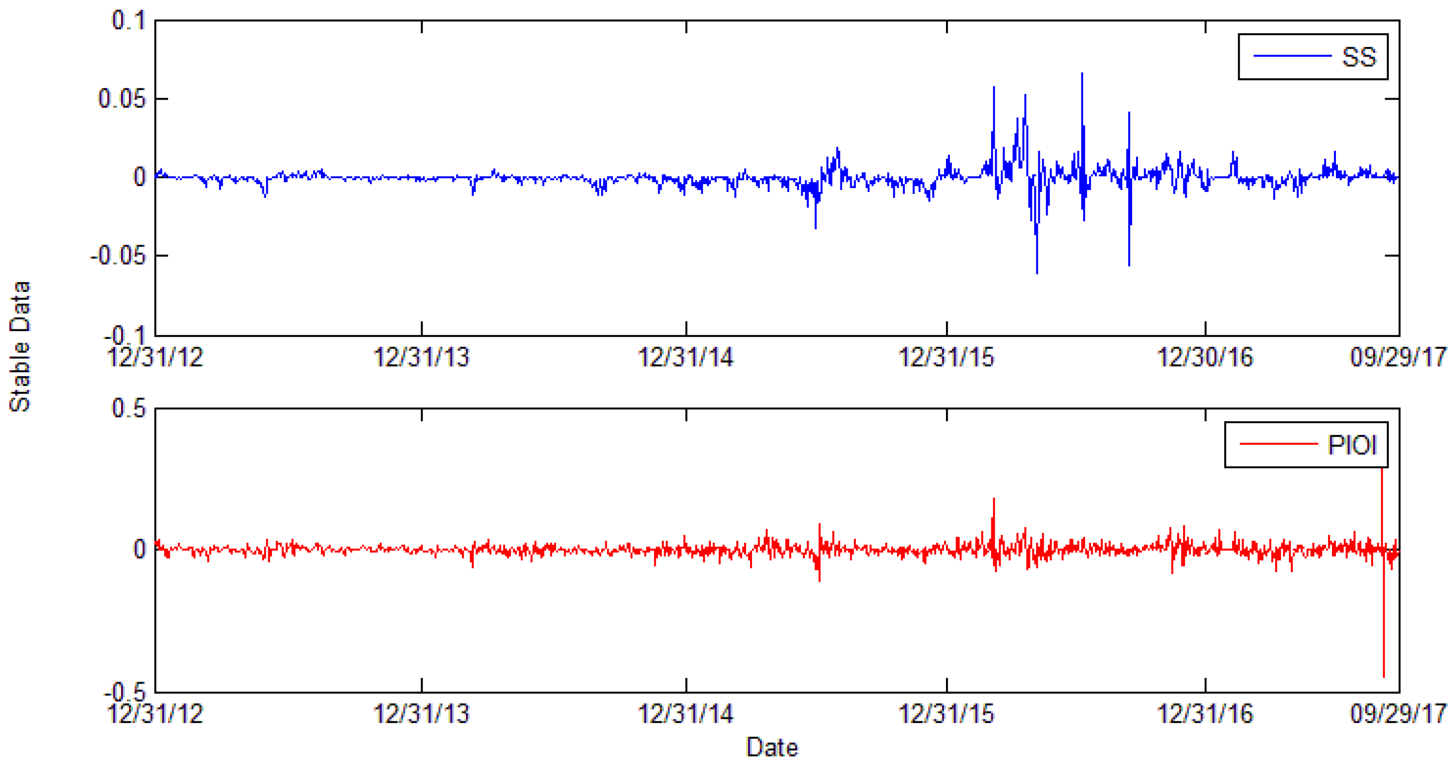
We calculate the log return of the price series and attain the stable data series. The scrap steel price and Platts iron ore index log return series are presented in
Figure 3. Midstream and downstream steel product prices log return series are presented in
Figure 4.
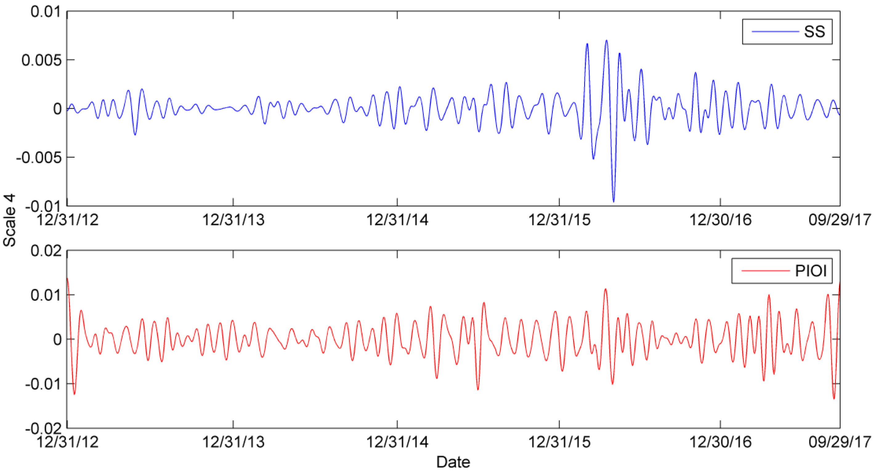
In
Figure 3, the blue line of SS represents the log return series of scrap steel. The red PIOI line represents the log return series of Platts iron ore index. The price of steel scrap fluctuates severely in the midterm of 2015 and the year 2016. The variation tendency of the Platts iron ore index is moderate. However, in the midterm of 2015 and early 2016, the index fluctuates a lot. In
Figure 4a,b, different colors represent different midstream and downstream steel products.
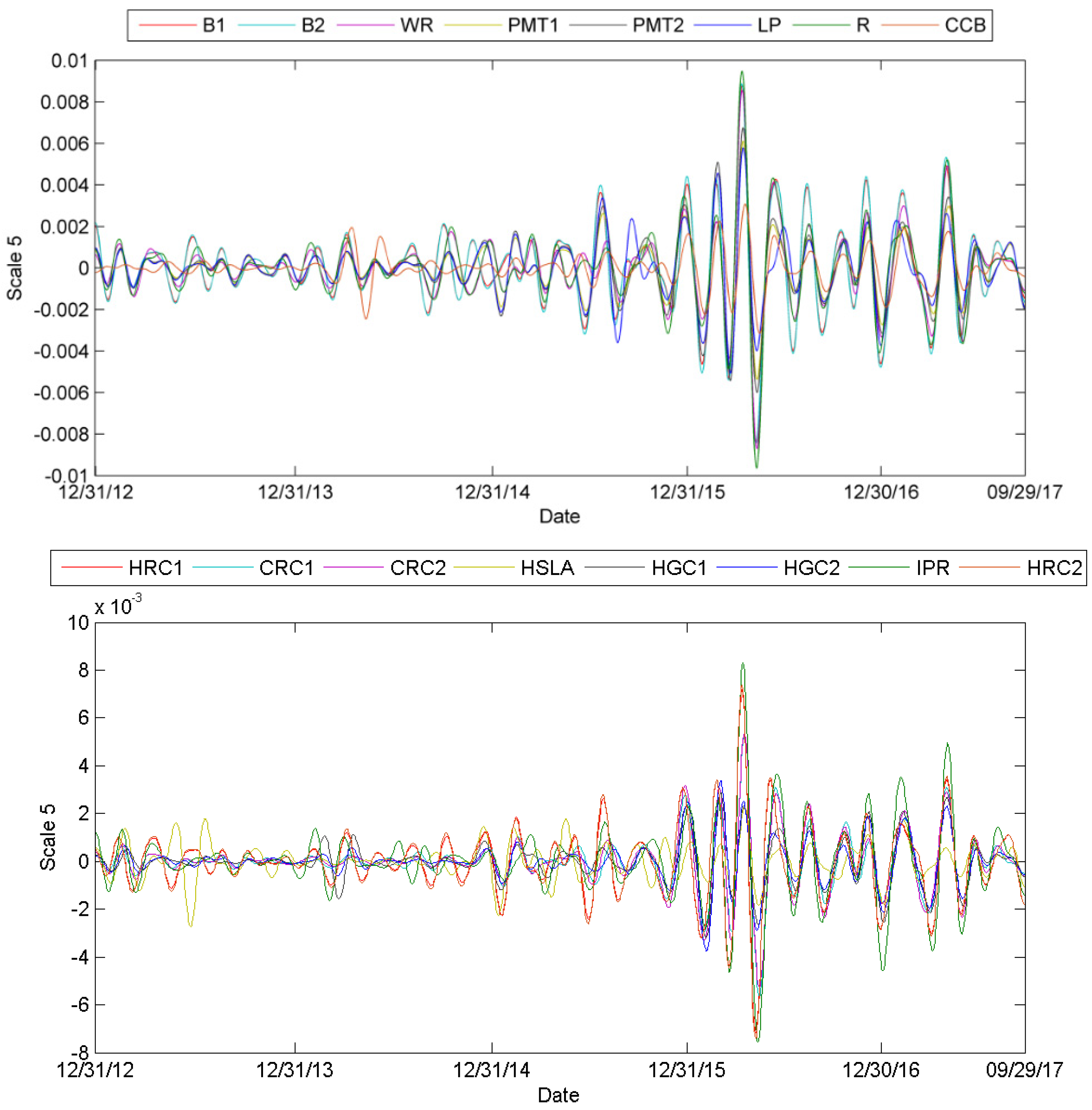
4.2. Wavelet Decomposition Comparison
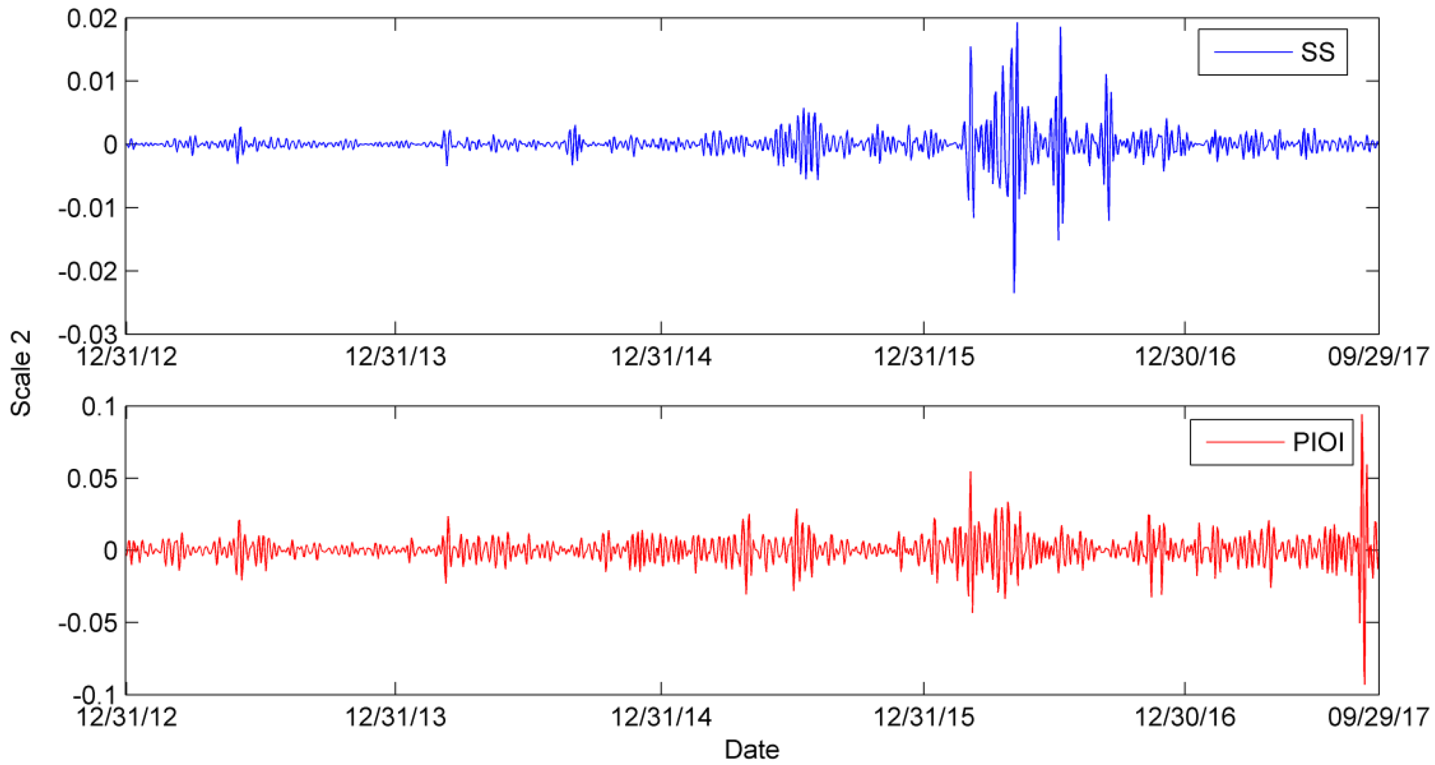
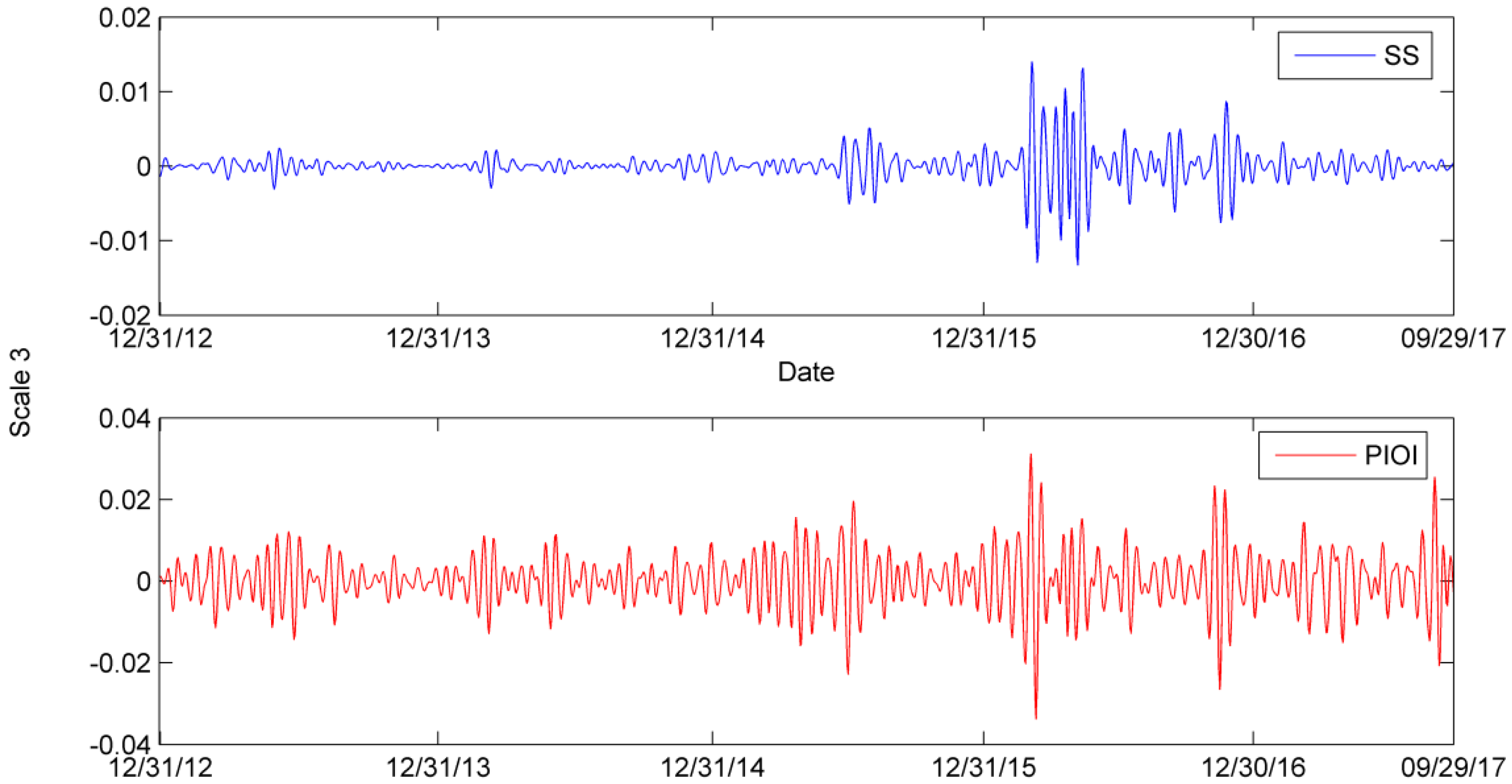
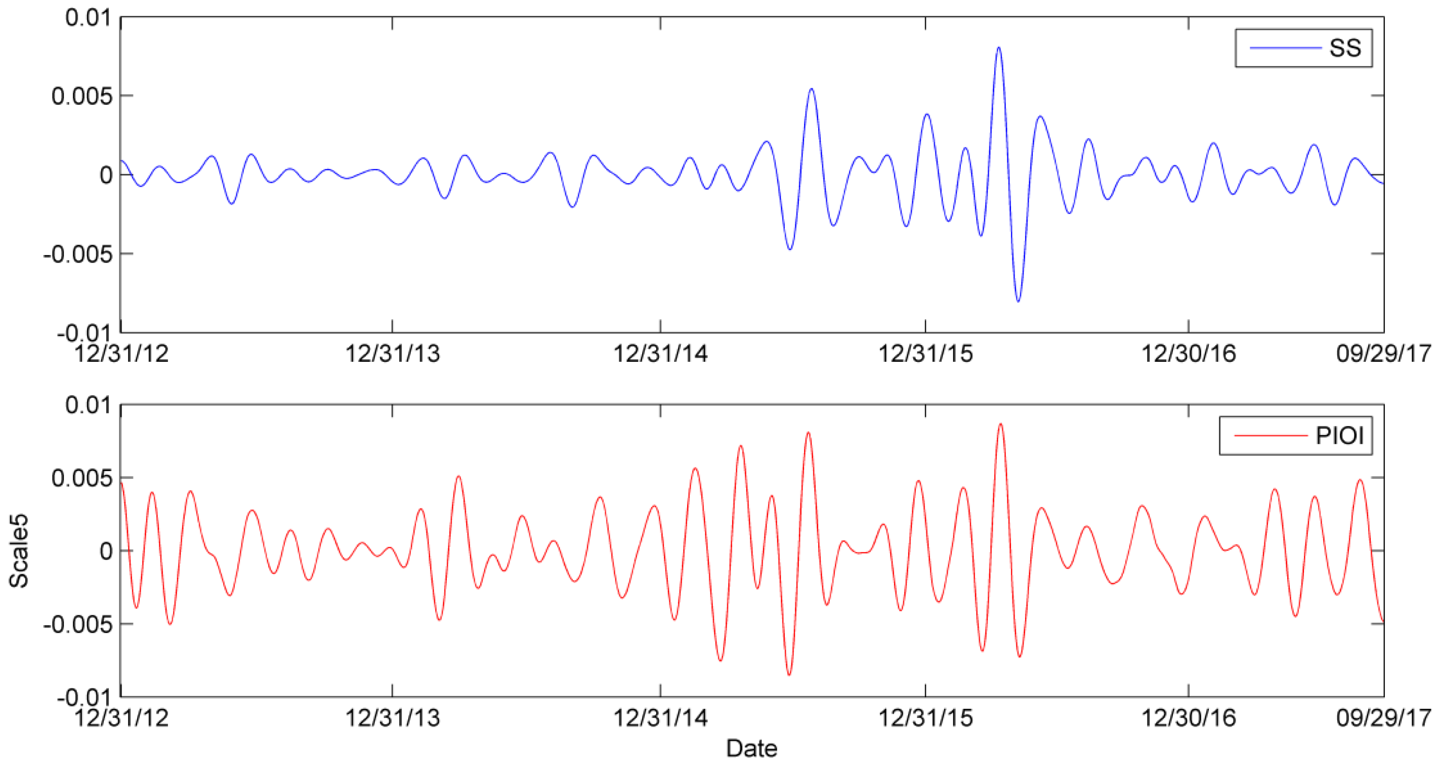
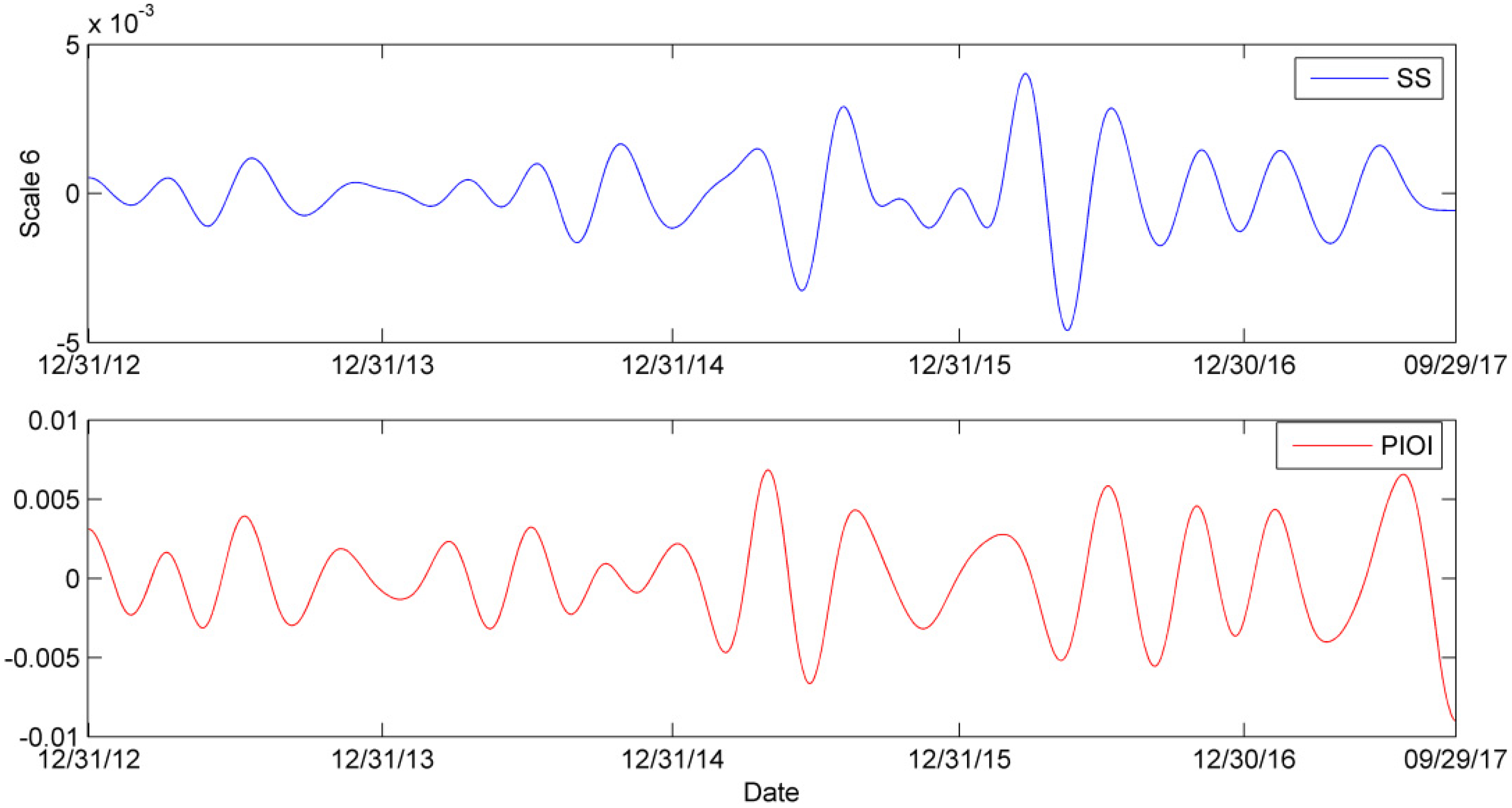
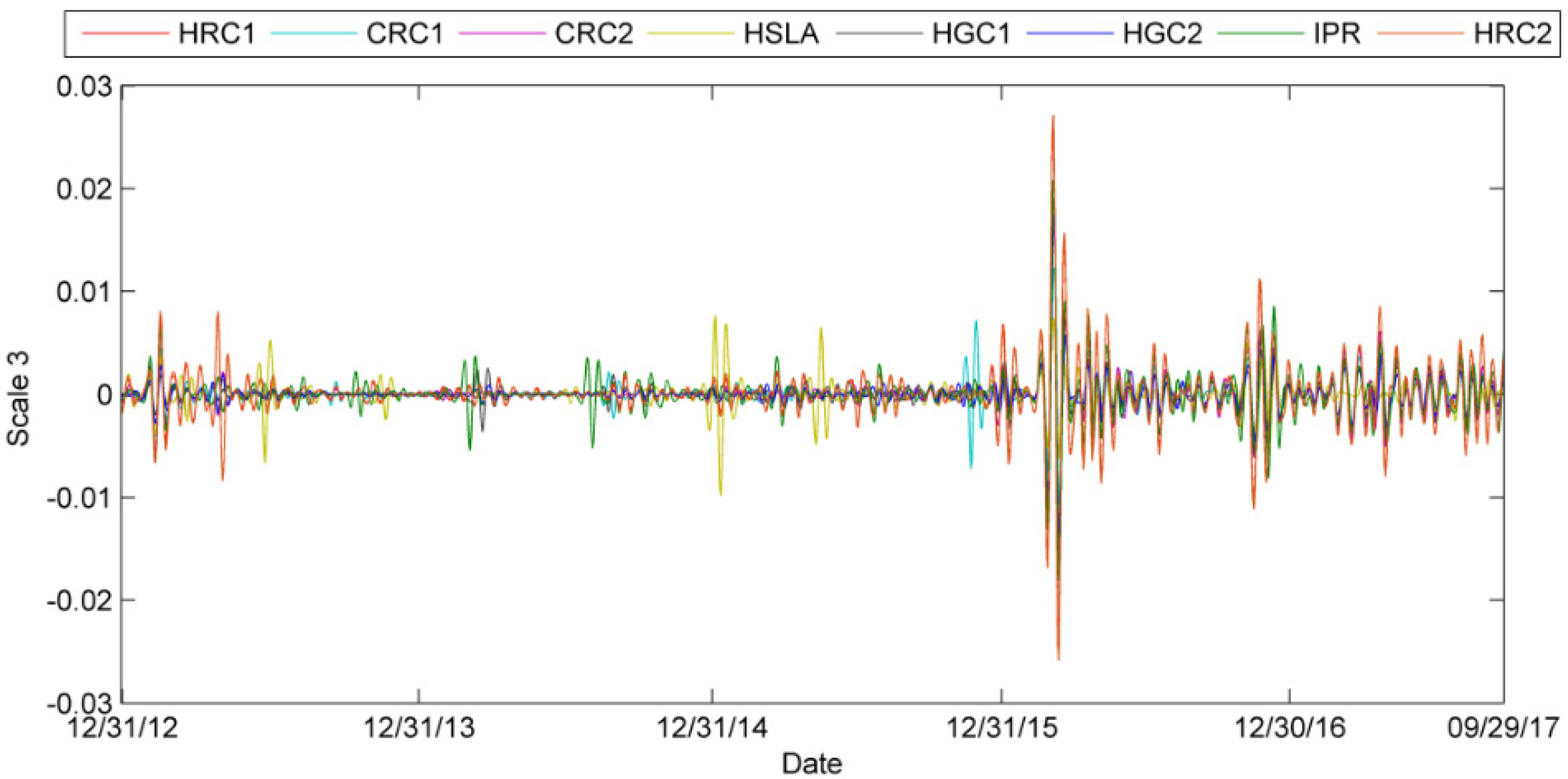
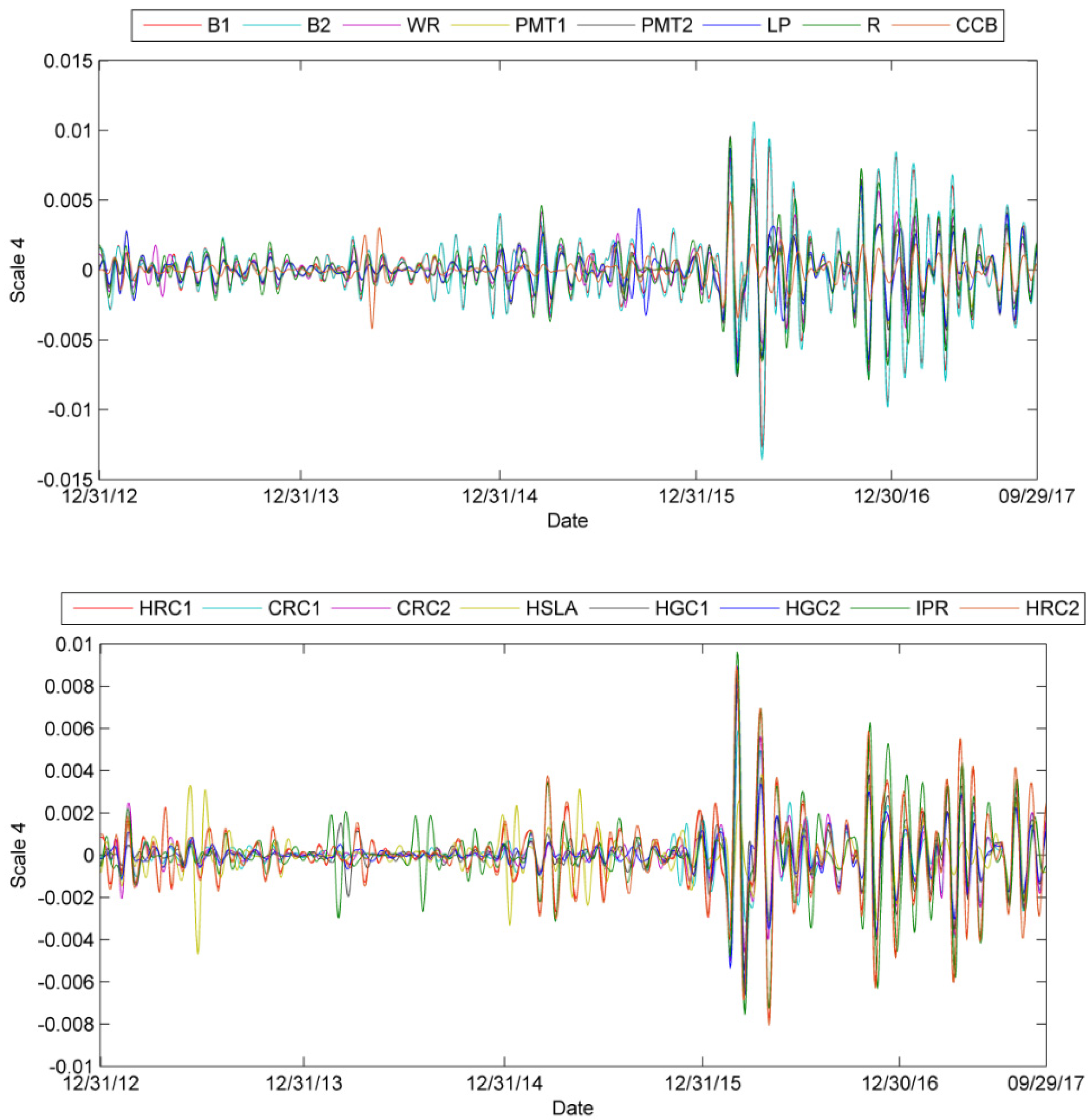
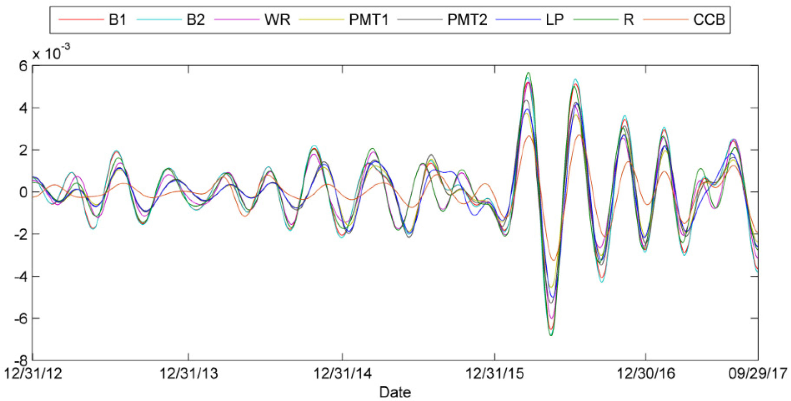
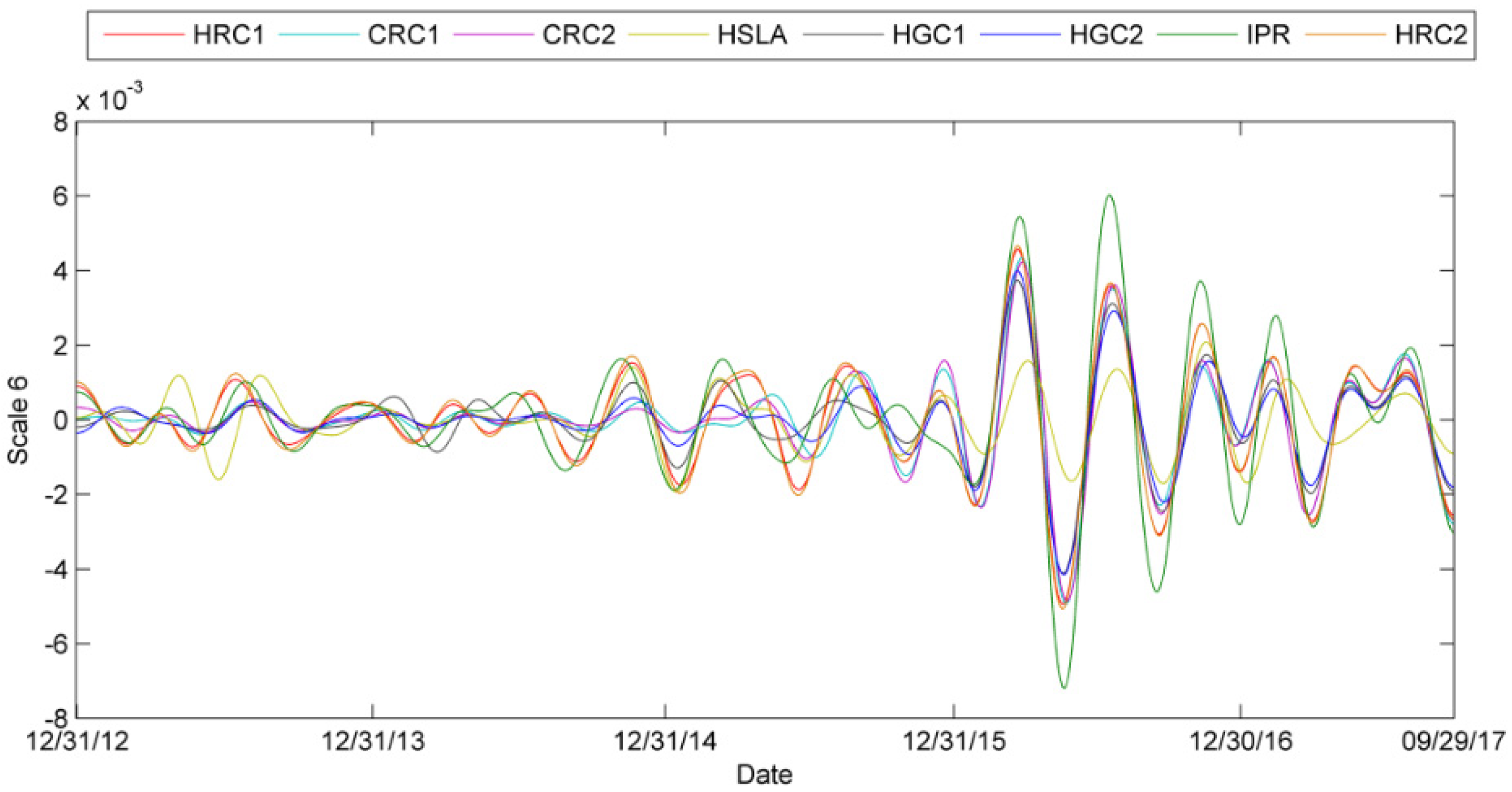
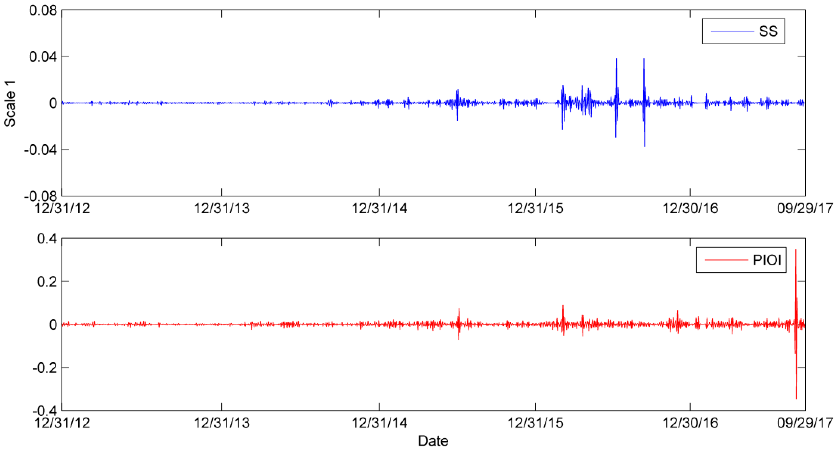
The wavelet decomposition method provides us with a perspective to capture the steel material and steel product price variation at different time scales. The detailed wavelet decomposition results are listed at
Appendix A.
In the
Appendix A, after decomposition of the original steel scrap price and Platts iron ore index, t in short-term, these two materials display various fluctuation patterns, while as the time scale grows, the fluctuation tendency gradually becomes concordant.
The steel product wavelet decomposition also exhibits similar features. This reflects that in the short-term, a particular steel product may fluctuate according to different reasons and represent various volatility tendencies. As time scale grows, those products are influenced by external factors as a whole steel market. Their fluctuation in the long run is in accordance with each.
However, there also exists distinguished features between steel products, especially in the short-term. In the scale 1 picture which depicts the price volatility within 2–4 days, these products fluctuate a lot at a particular date. This reflects that in the short-term, especially at 2–4 days period, these different steel products fluctuated according to their respective supply and demand rules.
Wavelet decomposition results reveal different time domain information for different market practitioners. For speculative investors who focus on short-term price fluctuations, it is critical to find the key price lead indicators because of the severely fluctuated markets in the short-term. For steelmaking companies, midterm and long-term price trend is the crucial time domain they should pay attention to. Their production and inventory decision are relatively long processes. Excessive attention on short-term results will disturb their normal operating activities. For policy makers, long-term time scale results should be paid more attention.
4.3. Price Lead-Lag Relationships Analysis
Then this study calculates the
p values of the Podobnik test and results show that all the cross-correlation at six time scales passes the test. The detailed lead-lag relationship coefficients and their lag orders are shown in
Table 3.
Table 3 shows the lag order results of PLRs between steel scrap and 16 steel products. The first column refers to the steel products code. The second column refers to the lag order results of original series. The last six columns refer to the lag order results of PLRs at six time scales. At original series, all lag orders of the PLRs are 0, which means that scrap steel price variation does not lead or lag the price fluctuation of steel products. Their price variation occurs in the same day. But at scale 1, the lag order results fluctuate a lot. PLR lag orders do not present unified rules that can be detected. This may be because at short-term, investors’ decisions are influenced by short-term market information and change quickly. Market volatility is high. At scale 2, most PLR lag orders become 0, which means scrap steel price and steel product prices fluctuate on the same day, but PLRs “Scrap steel to HRC1” and “Scrap steel to CRC1” steel present that scrap steel price lags HRC1 and CRC1 for 116 and 344 days respectively. This may because of the mediation of hot rolled coil and cold rolled coil products in the steel industry chain. These two steel product prices will in turn lead upstream materials. At midterm of scale 3 and scale 4, scrap steel price lags products Billet/Color coated board/Industrial round steel for one lag order. At long term, scrap steel price still lags billet products, but PLRs between scrap steel and other products differ according to steel products. In scale 5 (32–64 days), scrap steel price leads most steel products except Billet products/Low-alloy plate/Rebar/Color coated board/Industrial & P round steel. The leading lag order ranges from −4 to −1, which means at long term, scrap steel price leads these products for 32–256 days. What’s more, Low-alloy plate/Rebar/Color coated board/Industrial round steel prices fluctuates at the same lag order with scrap steel. At scale 6, in all 16 steel products, those products which are located the in upper stage of the industry chain, such as Billet/Wire rod/Plates of middle thickness/Rebar product prices lead the scrap steel price. Those which are located at a further downstream stage of the steel industry chain, such as Hot rolled coil/Cold rolled coil/High-strength low-alloy plate/Hot galvanized coil product prices lag scrap steel. These products endure a relatively long smelting process and their final application is more narrow than that of upper stage products. Therefore, their long-term price influence is weak.
The lead-lag relationship between Platts iron ore index and steel products also tells a similar story.
Table 4 shows the lag order results of PLRs between Platts iron ore index and 16 steel products. The first column refers to the steel products code. The second column refers to the lag order results of original series. The last six columns refer to the lag order results of PLRs at six time scales. The original series PLR lag order results are almost at −1, except the Color coated board product (at lag 785) and Cold rolled coil 0.5mm product (at lag 460). The results denote that Platts iron ore index usually fluctuates with the steel products at the same time. However, for Color coated board products and Cold rolled coil 0.5mm products, the Platts iron ore index usually lags them for more than one year. Moreover, Platts iron ore index and hot rolled coil products fluctuate at the same lag order. At scale 1, iron ore price variation lags 16 steel products, and the lag order results are extremely large. The reason may be the same as scrap steel’s scale 1 lag order results. In short-term, the investors’ decisions are influenced by short-term market information and change quickly. Market volatility is high. This trend continues to scale 2. In scale 2, Hot rolled coil 3 mm/Cold rolled coil 0.5 mm/High-strength low-alloy plate/Hot galvanized coil 1 mm products are still extremely large, but other products’ lag order results become normal. Iron ore price leads these steel products for one lag. At midterm scale 3 and scale 4, iron ore price leads almost all steel products except Cold rolled coil 0.5 mm product. On the one hand, results show the strong price lead influence of iron ore. On the other hand, Cold rolled coil product can in turn influence iron ore because of its importance in the industry chain. At long term scale 5, iron ore price leads all 16 steel products, and at scale 6, Billet products/Color coated board/Industrial & P round steel prices fluctuate at the same lag order with iron ore price, while other product prices fluctuations still lag the iron ore price. At long term, iron ore’s price no more lags Cold rolled coil products. Different from other products, PLR lag orders between iron ore index and Cold rolled coil product prices still fluctuate at long term and present extremely large results.
The lead-lag relationship results show that steel scrap price is tightly related to steel products, and their lead-lag relationship usually transmits with a lag order, namely one day. For Platts iron ore index, things are a bit different. Most steel products are related to the Platts index, while Color coated board products and Cold rolled coil 0.5 mm product prices lead the index by 785 and 460 days respectively. For other products, except that they have the largest lead-lag relation coefficients with Platts index at −1 lag order, they also present relatively strong lead relationships at other lag orders.
Comparing steel scrap to the Platts iron ore index, we can find that steel scrap price usually fluctuates with steel products at the same time. What is more, all the lead-lag relation is positive. However, for Platts iron ore index, its variation advances most steel products. This may be because iron ore, as the major material in the steel market, influences the steel scrap market and steel products market a lot. For steelmaking companies, they should focus more on iron ore price variations in the market because iron ore price variation leads most steel products for one day. This can help related companies regulate their production decision and hedge the price fluctuation risk in advance. However, Hot rolled coil product price variation lags the upstream iron ore price variation. This may because of hot rolled coil product’s vital mediation in the industry chain and it influences the upstream iron ore price in turn. This is a key price lead indicator for steel industries, because hot rolled coil product price leads the main steel materials.
What is more, the products (Color coated board, Cold rolled coil 0.5 mm, High-strength low-alloy plate) whose prices lead steel materials exist at the end of the steel industry chain.
Then we discuss the network results to find the structural price relationship in the steel market.
4.4. Complex Network Analysis
Then we establish steel products price lead-lag relationship network at each time scale and compare their network topological indicators. The industry chain compares two main steel materials.
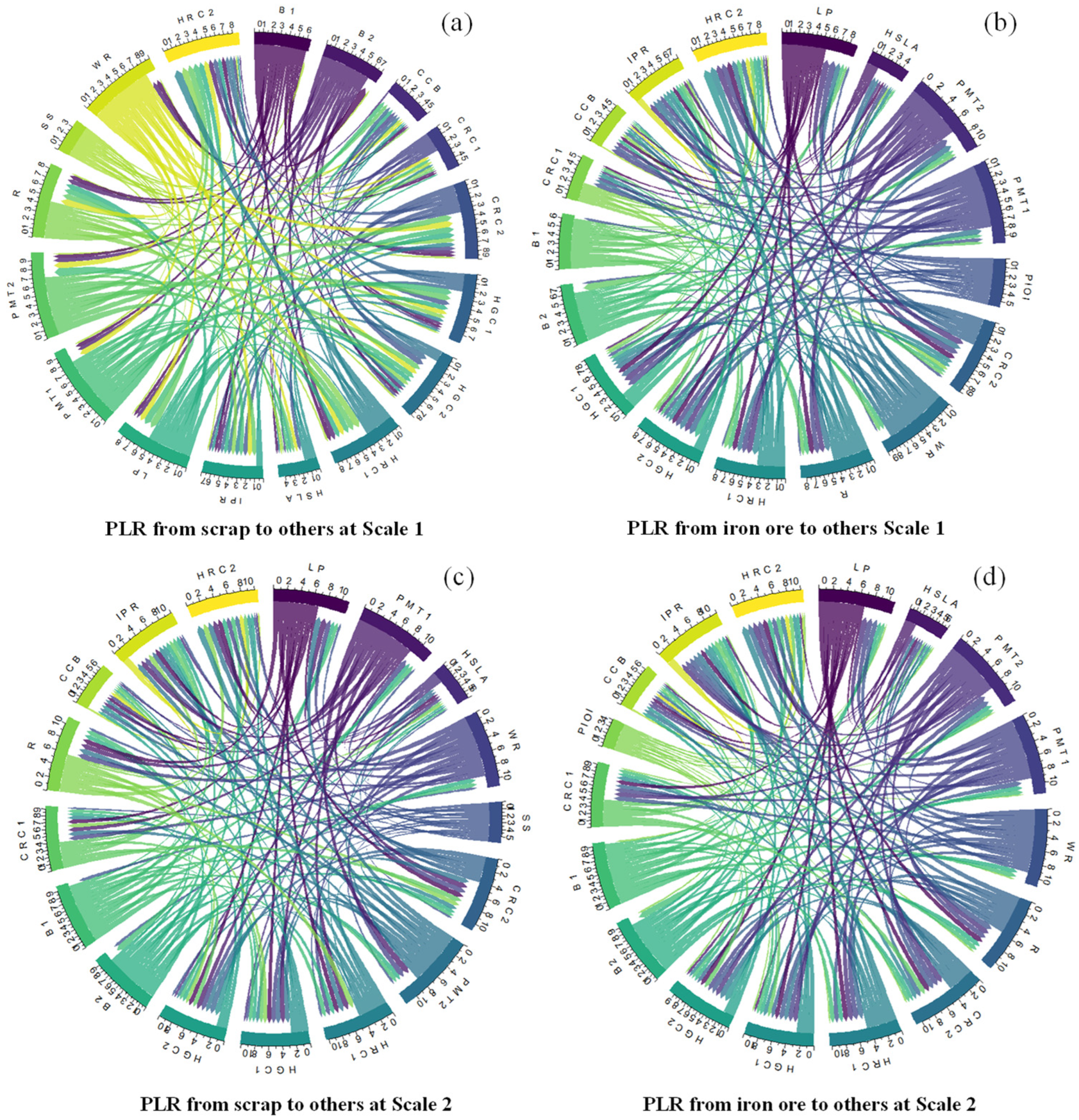
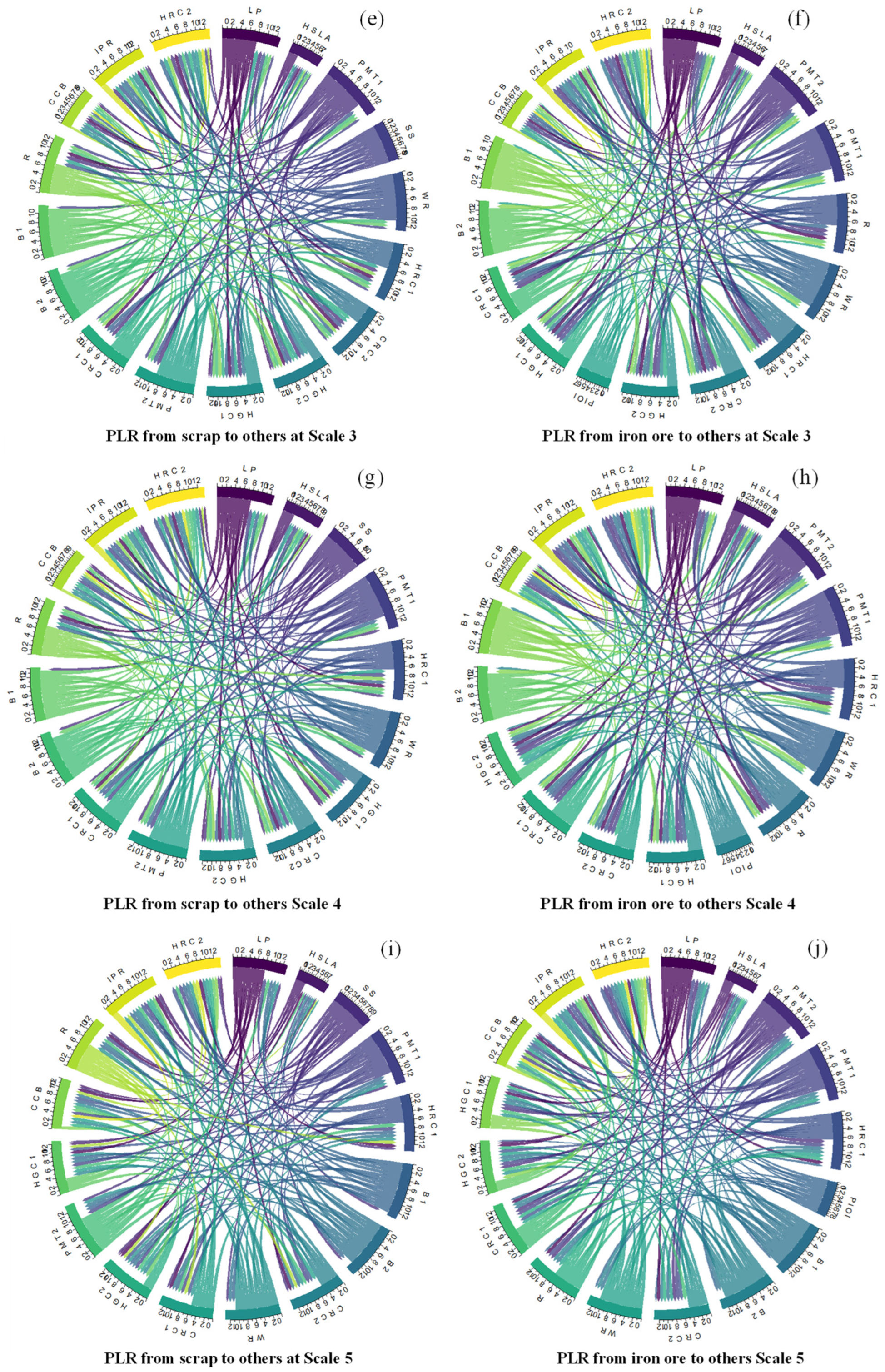
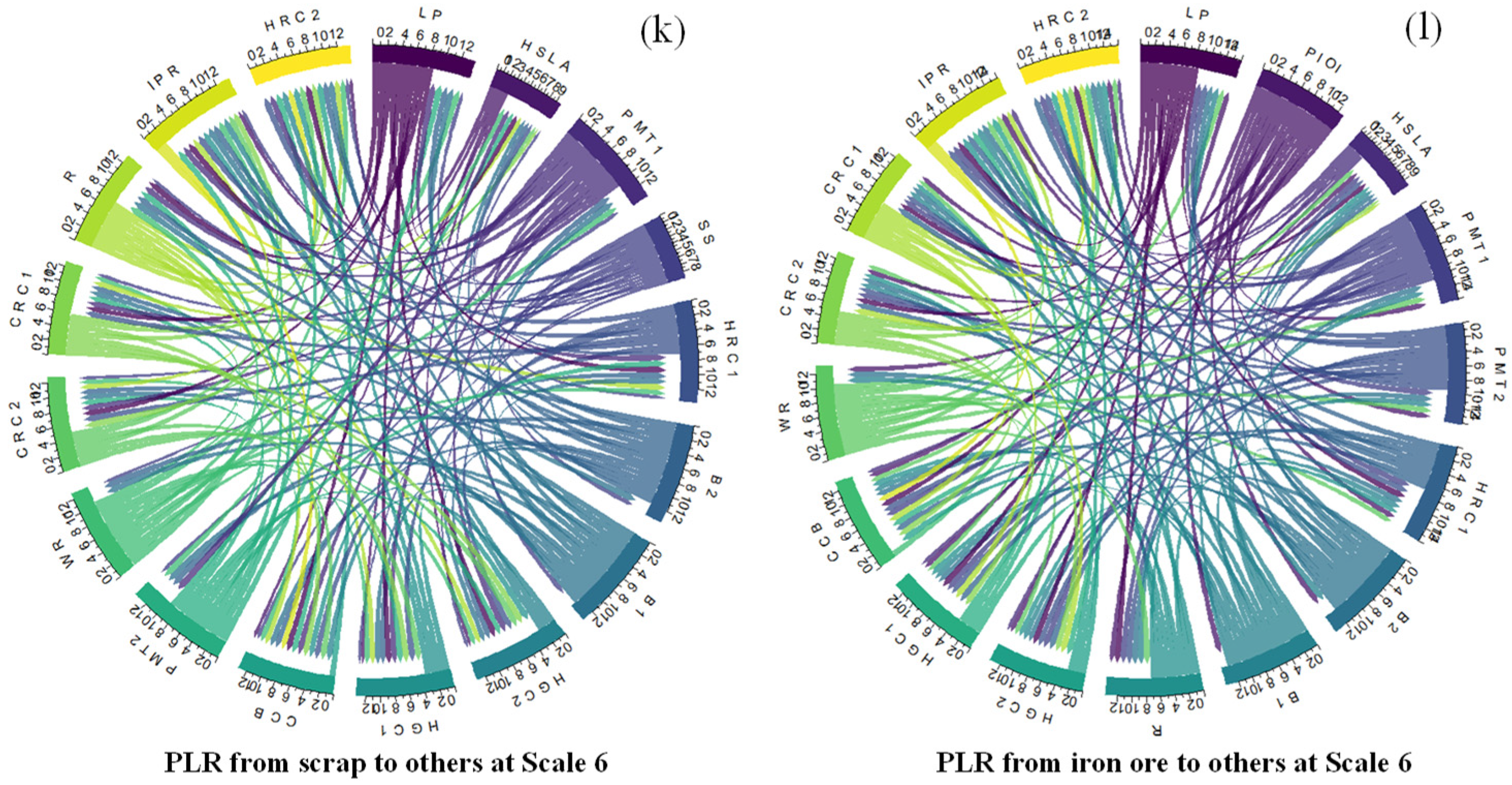
Figure 5 shows the PLRs from scrap steel and iron ore to other steel products at six time scales. Each color represents every steel product, and the flows with arrows between each entity represent the lead-lag relationship between steel products. The width of flow represents the number of lead-lag relationship coefficients between two steel products. Each arc is combined with two parts: those that lead relationships from one steel product to other products and those that lag relationships from other steel products to this entity.
Figure 5 reveals two trends in the PLRs from materials to steel products at different time scales. The first trend shows that as the time scale becomes longer, the PLR will be larger, which means that in long-term, there exists closer lead relationships from steel materials to steel products. In short-term scale 1, PLR from scrap to 16 steel products is −1.162, which means that price variation of scrap steel leads the downstream steel products and the summation of price lead relationship of all products is −1.162. At another short time scale 2, PLRs from scrap steel to downstream steel products have a large growth. The relationship coefficient is 5.946, while in long-term scale, the lead relationship is 8.903 (Scale 5) and 8.925 (Scale 6). The price lead relationship from iron ore to steel products also presents this trend. The price lead relationship in short-term is −3.895 (Scale 1) and 0.240 (Scale 2), while in long-term, the lead relationship is 8.532 (Scale 5) and 12.967 (Scale 6). The difference between short-term and long-term relationships may result from the relatively severe price fluctuation in short period. The market individuals cannot react to market fluctuations and enact corresponding measures in a short period. This causes a deviation between price signals and market fundamentals, so there presents the negative correlation between steel materials and products. As time scale grows and market individuals react to upstream price variation, the change in product price in the whole industrial chain shows a positive correlation trend. Similar results with the wavelet transform analysis are presented which prove the closer lead relationship from steel materials to steel products in long-term. For steelmaking companies, midterm and long-term price trend is the crucial time domain they should pay attention to. Their production and inventory decision are relatively long processes. Excessive attention on short-term results will disturb their normal operating activities.
The second trend shows that iron ore has tighter PLRs than downstream steel products at the shortest time scale and longest time scale, while scrap steel has tighter PLRs with downstream steel products at a relative midterm period. Iron ore price has a tight PLR with the downstream steel products in short-term of 2–4 days (−3.895) and long-term of 64–128 days (12.967). Scrap steel prices influence the downstream steel price at midterm of 8–32 days (7.557 and 6.599). At scale 2 (0.240) for short-term and scale 5 (8.532) for long-term, scrap steel also has tighter price relationships with steel products than iron ore.
Table 5 shows the network indicator calculation results of each network.
Table 5 shows the weighted outdegree and out closeness centrality indicator of 12 networks. Each row shows the two network indicators at the scrap steel PLRs network and iron ore PLRs network at each time scale. The network indicator results show the same trends from the network analysis in
Figure 5.
According to the out-closeness centrality indicator results, on the one hand, as the time scale grows, centrality of two materials declines gradually. In short-term, midterm and long-term scales, the average lead centrality from scrap steel materials to steel products is 0.211 (Scale 1/Scale 2), 0.106 (Scale 3/Scale 4), and 0.090 (Scale 5/Scale 6), while the indicators of iron ore are 0.207 (Scale 1/Scale 2), 0.129 (Scale 3/Scale 4) and 0.090 (Scale 5/Scale 6). This reflects that as the time scale grows, the network distance between materials and end-use steel products becomes short, which means the price variation of two materials is easier to impose on each downstream product. In short-term, price variation of steel materials is reflected in the iron ore and scrap steel spot trading market. Because of the time lag effects, steel products at midstream and downstream react to the market information slowly. As time scale grows, in the midterm and long-term, market individuals at midstream and downstream begin to regulate their supply and demand based on price information. This implication is consistent with the market activities. Then the price fluctuation in upstream materials transmits to downstream products. Therefore, in long-term, two steel materials are easier to lead end-use steel products. For steel companies, it is important to focus on this price transmission process, especially this vertical transmission from different segments of the industry chain. Little attention is usually paid to the horizontal regional price transmission activities. In long-term, upstream steel material prices are easier to lead downstream steel products. This indicates that for policy makers, policy regulation targets should be unambiguous, but policy regulation processes should be flexible. Policy regulation enacted by policy makers is aimed at long-term industry development and focuses on long-term price information. Therefore, the policy target should be unambiguous. In long-term, upstream steel material prices are easier to lead downstream steel products, but the short-term and midterm price trend may fluctuate and influence the speculative investors and steel companies’ decisions. When making long-term policies, public sectors should take market individuals’ response into consideration. Its policy regulation process should be flexible.


