
Using Background Knowledge from Preceding Studies for Building a Random Forest Prediction Model: A Plasmode Simulation Study


Abstract
:1. Introduction
2. Materials and Methods
2.1. Methods to Train Models
2.1.1. Logistic Regression
2.1.2. Random Forest
2.2. Methods to Evaluate Performance of Model Predictions
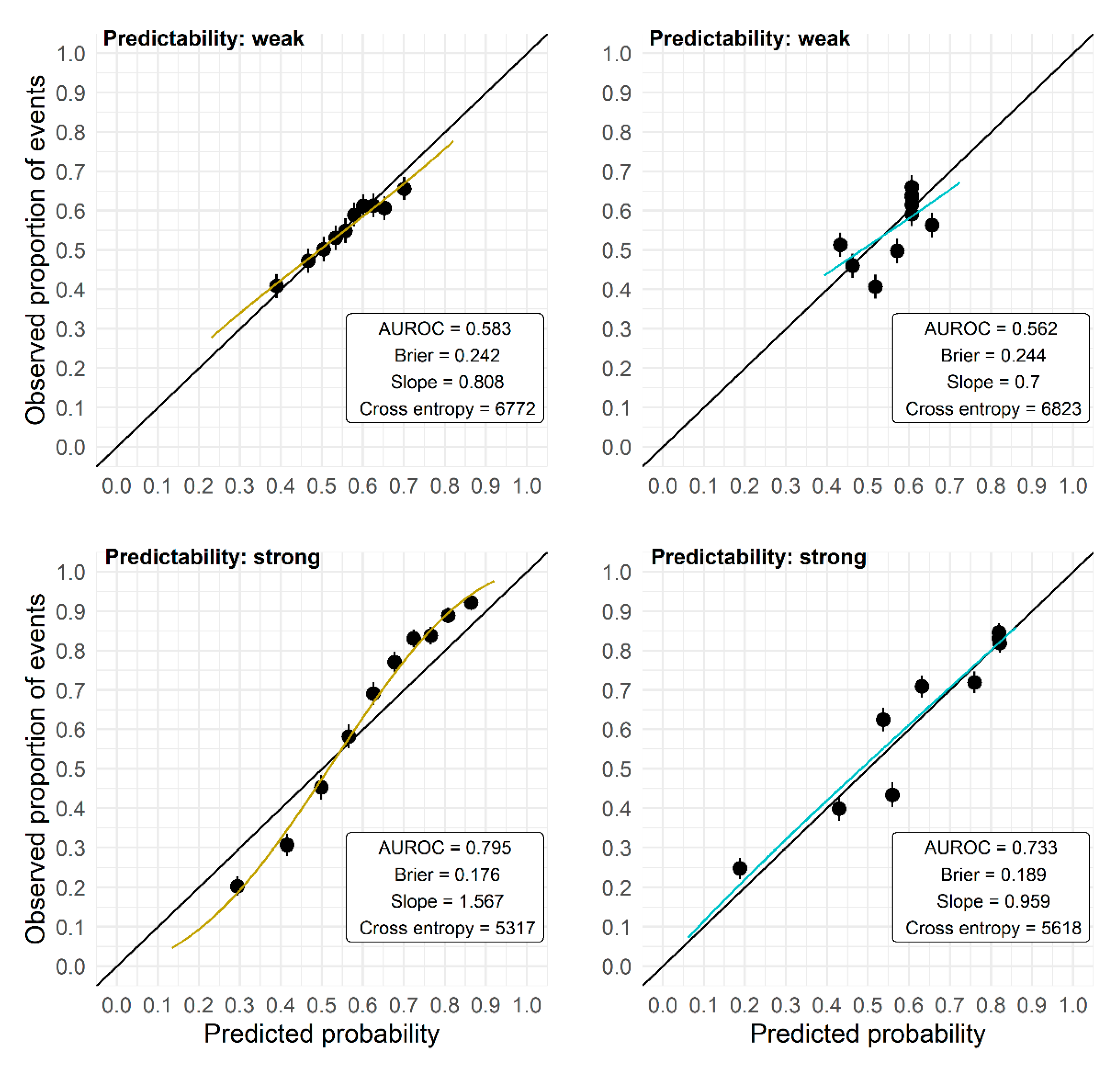
- Area under the receiver operating characteristic curve (AUROC) or concordance statistic: ; ideal value 1
- Brier score: ; ideal value 0
- Calibration slope: slope of a logistic regression of on ; ideal value 1
- Cross-entropy: ; ideal value 0
2.3. Motivating Study
2.4. Setup of the Plasmode Simulation Study
2.4.1. Aims
2.4.2. Data Generating Mechanisms
2.4.3. Estimands and Other Targets
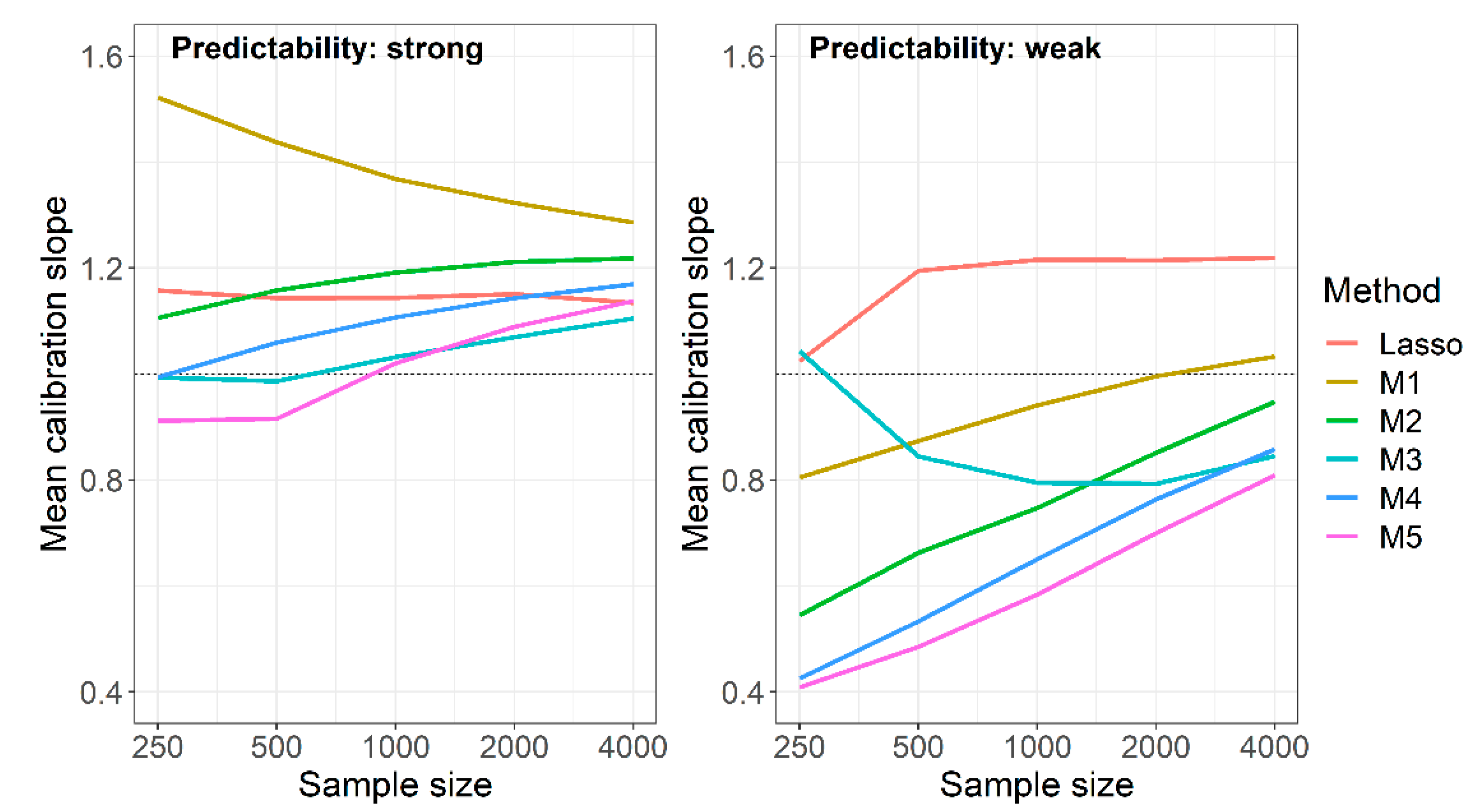
2.4.4. Methods
- All variables (M1, naïve RF);
- Those variables that were selected by the Lasso in the preceding study 1 (M2);
- Those variables that were selected by the Lasso in preceding study 1 and univariate selection in preceding study 2 (M3);
- Those variables that were selected by the Lasso in preceding study 1 or univariate selection in preceding study 2 (M4);
- Those variables that were selected by the “better performing” model. This model was determined by applying the model from preceding study 1 (Lasso) and the model from preceding study 2 (univariate selection) unchanged on the data of the current study and comparing the resulting area under the ROC. The model with the higher AUROC was considered the “better performing” model. (M5)
- If for M2 no variables were selected, we used all candidate predictors instead (no preceding variable selection);
- If for M3 the intersection was the empty set, we used the result of M4;
- If for M4 the union of the variable sets was the empty set, we used all predictors;
- If for M5 one of the models was empty, we used the predictors from the other model as input; if none of the preceding studies selected any predictors we used all predictors in the current study.
2.4.5. Performance Measures
2.4.6. Pilot Study
2.4.7. Software
3. Results
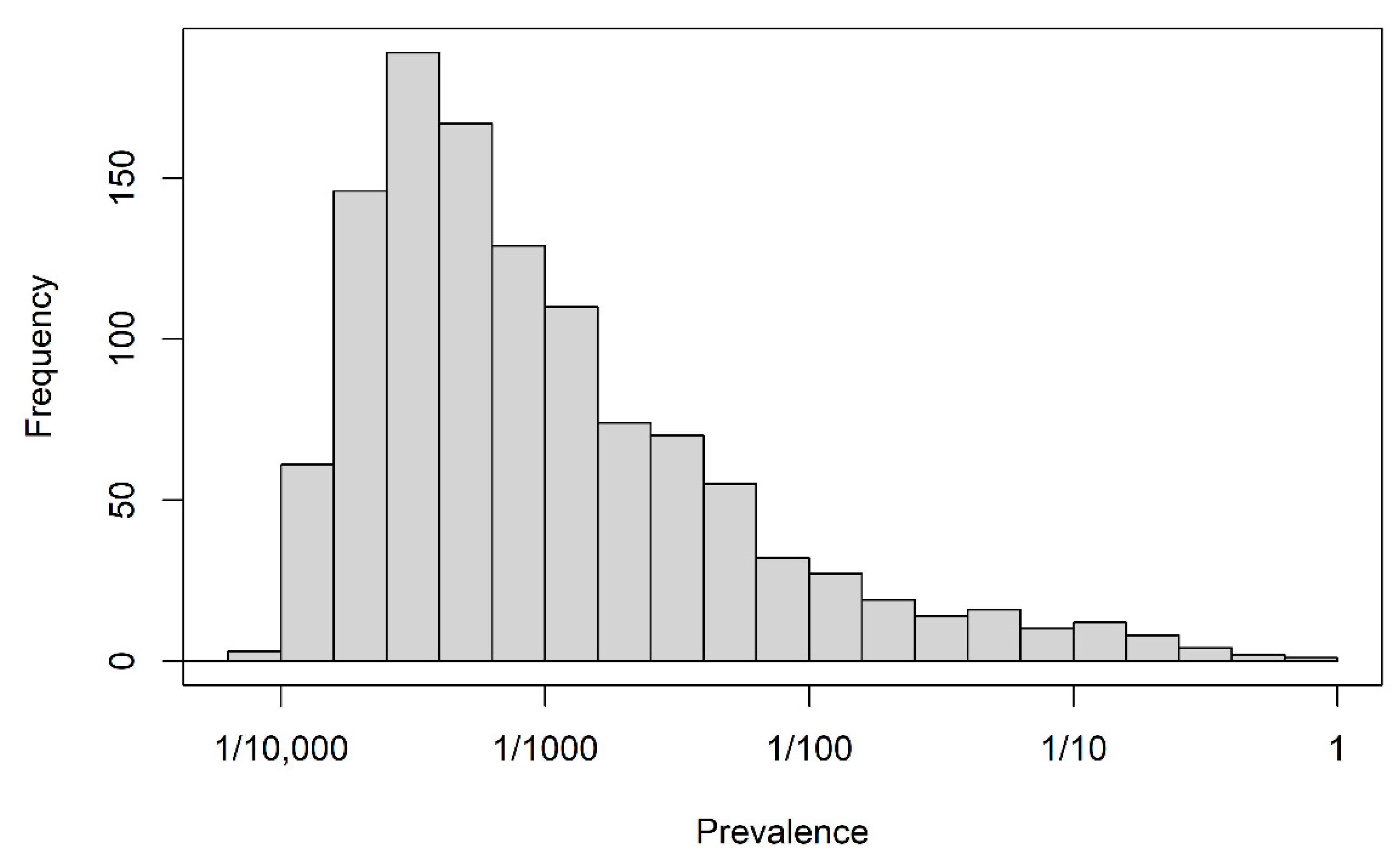
3.1. Descriptives
3.1.1. Number of Candidate Predictors
3.1.2. Selected Predictors in the Preceding Studies
3.2. Comparison of Performance
4. Discussion
5. Conclusions
Supplementary Materials
Author Contributions
Funding
Data Availability Statement
Acknowledgments
Conflicts of Interest
References
- Hernán, M.A.; Hsu, J.; Healy, B. A second chance to get causal inference right: A classification of data science tasks. Chance 2019, 32, 42–49. [Google Scholar] [CrossRef] [Green Version]
- Shmueli, G. To Explain or to Predict? Stat. Sci. 2010, 25, 289–310. [Google Scholar] [CrossRef]
- Hemingway, H.; Croft, P.; Perel, P.; Hayden, J.A.; Abrams, K.; Timmis, A.; Briggs, A.; Udumyan, R.; Moons, K.G.M.; Steyerberg, E.W.; et al. Prognosis research strategy (PROGRESS) 1: A framework for researching clinical outcomes. BMJ 2013, 346, e5595. [Google Scholar] [CrossRef] [Green Version]
- Breiman, L. Statistical modelling: The two cultures. Stat. Sci. 2001, 16, 199–231. [Google Scholar] [CrossRef]
- Hastie, T.; Tibshirani, R.; Friedman, J. The Elements of Statistical Learning, 2nd ed.; Springer: New York, NY, USA, 2009; ISBN 978-0-387-84857-0. [Google Scholar]
- Tibshirani, R. Regression Shrinkage and Selection via the Lasso. J. R. Stat. Soc. Ser. B 1996, 58, 267–288. [Google Scholar] [CrossRef]
- Bühlmann, P. Boosting for high-dimensional linear models. Ann. Stat. 2006, 34, 559–583. [Google Scholar] [CrossRef] [Green Version]
- Harrell, F.E. Regression Modelling Strategies, 2nd ed.; Springer: New York, NY, USA, 2015; ISBN 978-3-319-19424-0. [Google Scholar]
- Royston, P.; Sauerbrei, W. Multivariable Model-Building: A Pragmatic Approach to Regression Analysis Based on Fractional Polynomials for Modelling Continuous Variables, 1st ed.; John Wiley & Sons Ltd.: Chichester, UK, 2008; pp. 115–150. ISBN 78-0-470-02842-1. [Google Scholar]
- Heinze, G.; Wallisch, C.; Dunkler, D. Variable selection—A review and recommendation for the practicing statistician. Biom. J. 2018, 60, 431–449. [Google Scholar] [CrossRef] [Green Version]
- Sauerbrei, W.; Perperoglou, A.; Schmid, M.; Abrahamowicz, M.; Becher, H.; Dunkler, D.; Harrel, F.E.; Royston, P.; Georg Heinze for TG2 of the STRATOS Initiative. State of the art in selection of variables and functional forms in multivariable analysis—Outstanding issues. Diagn. Progn. Res. 2020, 4, 3. [Google Scholar] [CrossRef] [Green Version]
- van der Ploeg, T.; Austin, P.C.; Steyerberg, E.W. Modern modelling techniques are data hungry: A simulation study for predicting dichotomous endpoints. BMC Med. Res. Methodol. 2014, 14, 137. [Google Scholar] [CrossRef] [Green Version]
- Bergerson, L.C.; Glad, I.K. Weighted Lasso with Data Integration. Stat. Appl. Genet. Mol. Biol. 2011, 10, 1–29. [Google Scholar] [CrossRef]
- Wright, M.N.; Ziegler, A. Ranger: A Fast Implementation of Random Forests for High Dimensional Data in C++ and R. J. Stat. Softw. 2017, 77, 1–17. [Google Scholar] [CrossRef] [Green Version]
- Sun, G.W.; Shook, T.L.; Kay, G.L. Inappropriate Use of Bivariable Analysis to Screen Risk Factors for Use in Multivariable Analysis. J. Clin. Epidemiol. 1996, 49, 907–916. [Google Scholar] [CrossRef]
- Heinze, G.; Dunkler, D. Five myths about variable selection. Transpl. Int. 2017, 30, 6–10. [Google Scholar] [CrossRef]
- Breiman, L. Random forests. Mach. Learn. 2001, 45, 5–32. [Google Scholar] [CrossRef] [Green Version]
- Malley, J.D.; Kruppa, J.; Dasgupta, A.; Malley, K.G.; Ziegler, A. Probability machines: Consistent probability estimation using nonparametric learning machines. Methods Inf. Med. 2012, 51, 74–81. [Google Scholar] [CrossRef]
- Strobl, C.; Boulesteix, A.L.; Zeileis, A.; Hothorn, T. Bias in random forest variable importance measures: Illustrations, sources and a solution. BMC Bioinform. 2007, 8, 25. [Google Scholar] [CrossRef] [Green Version]
- Steyerberg, E.W.; Vickers, A.J.; Cook, N.R.; Gerds, T.; Gonen, M.; Obuchowski, N.; Pencina, M.J.; Kattan, M.W. Assessing the performance of prediction models: A framework for traditional and novel measures. Epidemiology 2010, 21, 128–138. [Google Scholar] [CrossRef] [Green Version]
- Tian, Y.; Reichardt, B.; Dunkler, D.; Hronsky, M.; Winkelmayer, W.C.; Bucsics, A.; Strohmaier, S.; Heinze, G. Comparative effectiveness of branded vs. generic versions of antihypertensive, lipid-lowering and hypoglycemic substances: A population-wide cohort study. Sci. Rep. 2020, 10, 5964. [Google Scholar] [CrossRef] [Green Version]
- WHO Collaborating Centre for Drug Statistics Methodology. Guidelines for ATC Classification and DDD Assignment 2012; Norwegian Institute of Public Health: Oslo, Norway, 2011; ISBN 978-82-8082-477-6. [Google Scholar]
- Morris, T.P.; White, I.R.; Crowther, M.J. Using simulation studies to evaluate statistical methods. Stat. Med. 2019, 38, 2074–2102. [Google Scholar] [CrossRef] [Green Version]
- Friedman, J.; Hastie, T.; Tibshirani, R. Regularization Paths for Generalized Linear Models via Coordinate Descent. J. Stat. Softw. 2010, 33, 1–22. [Google Scholar] [CrossRef] [Green Version]
- Van Calster, B.; van Smeden, M.; De Cock, B.; Steyerberg, E.W. Regression shrinkage methods for clinical prediction models do not guarantee improved performance: Simulation study. Stat. Methods Med. Res. 2020, 29, 3166–3178. [Google Scholar] [CrossRef] [PubMed]
- Van Calster, B.; McLernon, D.J.; van Smeden, M.; Wynants, L.; Steyerberg, E.W.; on behalf of Topic Group ‘Evaluating Diagnostic Tests and Prediction Models’ of the STRATOS Initiative. Calibration: The Achilles heel of predictive analytics. BMC Med. 2019, 17, 230. [Google Scholar] [CrossRef] [PubMed] [Green Version]
- Wynants, L.; Van Calster, B.; Collins, G.S.; Riley, R.D.; Heinze, G.; Schuit, E.; Bonten, M.M.J.; Dahly, D.L.; Damen, J.A.A.; Debray, T.P.A.; et al. Prediction models for diagnosis and prognosis of covid-19: Systematic review and critical appraisal. BMJ 2020, 369, m1328. [Google Scholar] [CrossRef] [PubMed] [Green Version]
- Haller, M.C.; Aschauer, C.; Wallisch, C.; Leffondré, K.; van Smeden, M.; Oberbauer, R.; Heinze, G. Prediction models for living organ transplantation are poorly developed, reported, and validated: A systematic review. J. Clin. Epidemiol. 2022, 145, 126–135. [Google Scholar] [CrossRef] [PubMed]
- Collins, G.S.; Reitsma, J.B.; Altman, D.G.; Moons, K.G. Transparent reporting of a multivariable prediction model for individual prognosis or diagnosis (TRIPOD): The TRIPOD statement. BMJ 2015, 350, g7594. [Google Scholar] [CrossRef] [Green Version]
- Moons, K.G.M.; Wolff, R.F.; Riley, R.D.; Whiting, P.F.; Westwood, M.; Collins, G.S.; Reitsma, J.B.; Kleijnen, J.; Mallett, S. PROBAST: A tool to assess risk of bias and applicability of prediction model studies: Explanation and elaboration. Ann. Intern. Med. 2019, 170, W1–W33. [Google Scholar] [CrossRef] [PubMed] [Green Version]
- Hafermann, L.; Becher, H.; Herrmann, C.; Klein, N.; Heinze, G.; Rauch, G. Statistical model building: Background “knowledge” based on inappropriate preselection causes misspecification. BMC Med. Res. Methodol 2021, 21, 196. [Google Scholar] [CrossRef]
- Zou, H.; Hastie, T. Regularization and Variable Selection via the Elastic Net. J. R. Stat. Soc. B. 2005, 67, 301–320. [Google Scholar] [CrossRef] [Green Version]
- Heinze, G.; Hronsky, T.; Reichardt, B.; Baumgärtel, C.; Müllner, M.; Bucsics, A.; Winkelmayer, W.C. Potential Savings in Prescription Drug Costs for Hypertension, Hyperlipidemia, and Diabetes Mellitus by Equivalent Drug Substitution in Austria: A Nationwide Cohort Study. Appl. Health Econ. Health Policy 2014, 13, 193–205. [Google Scholar] [CrossRef]
- Heinze, G.; Jandeck, L.M.; Hronsky, M.; Reichardt, B.; Baumgärtel, C.; Bucsics, A.; Müllner, M.; Winkelmayer, W.C. Prevalence and determinants of unintended double medication of antihypertensive, lipid-lowering, and hypoglycemic drugs in Austria: A nationwide cohort study. Pharmacoepidemiol. Drug Saf. 2015, 25, 90–99. [Google Scholar]
- Jandeck, L.M. Populationsweite Utilisationsuntersuchung in den chronischen Krankheitsbildern Hypertonie, Hyperlipidämie und Typ 2 Diabetes Mellitus. Inaugural Dissertation, Ruhr-Universität Bochum, Bochum, Germany, 2014. [Google Scholar]


| Predictability | N | Lasso | Univariate Selection | Union of Lasso and Univariate Selection | Intersection of Lasso and Univariate Selection |
|---|---|---|---|---|---|
| Strong | 4000 | 117 [58, 196] | 210 [175, 228] | 277 [220, 346] | 50 [33, 69] |
| 2000 | 103 [47, 178] | 111 [105, 118] | 179 [129, 246] | 35 [22, 51] | |
| 1000 | 75 [29, 139] | 55 [51, 60] | 109 [67, 167] | 22 [15, 31] | |
| 500 | 56 [11, 112] | 27 [25, 30] | 71 [32, 130] | 12 [8, 17] | |
| 250 | 33 [9, 89] | 14 [11, 15] | 41 [17, 95] | 6 [1, 11] | |
| Weak | 4000 | 68 [22, 152] | 84 [60, 102] | 130 [81, 212] | 22 [13, 35] |
| 2000 | 55 [11, 151] | 52 [35, 76] | 93 [56, 174] | 15 [7, 25] | |
| 1000 | 37 [0, 131] | 30 [17, 45] | 60 [29, 144] | 8 [0, 18] | |
| 500 | 21 [0, 88] | 17 [4, 29] | 34 [4, 96] | 3 [0, 10] | |
| 250 | 14 [0, 76] | 8 [0, 15] | 20 [2, 81] | 1 [0, 7] |
| Predictability | Sample Size | Lasso | M1 | M2 | M3 | M4 | M5 |
|---|---|---|---|---|---|---|---|
| Strong | 4000 | 5081 | 5050 | 4962 | 4990 | 5024 | 5045 |
| 2000 | 5152 | 5116 | 5034 | 5073 | 5090 | 5122 | |
| 1000 | 5253 | 5195 | 5126 | 5185 | 5178 | 5236 | |
| 500 | 5396 | 5296 | 5255 | 5368 | 5298 | 5419 | |
| 250 | 5599 | 5428 | 5455 | 5609 | 5466 | 5581 | |
| Weak | 4000 | 6621 | 6595 | 6606 | 6633 | 6625 | 6644 |
| 2000 | 6660 | 6624 | 6662 | 6688 | 6677 | 6707 | |
| 1000 | 6713 | 6662 | 6733 | 6751 | 6749 | 6796 | |
| 500 | 6777 | 6711 | 6816 | 6839 | 6850 | 6897 | |
| 250 | 6846 | 6767 | 6894 | 6957 | 6959 | 6987 |
| Predictability | Sample Size | Lasso | M1 | M2 | M3 | M4 | M5 |
|---|---|---|---|---|---|---|---|
| Strong | 4000 | 0.809 | 0.812 | 0.818 | 0.813 | 0.811 | 0.809 |
| 2000 | 0.803 | 0.807 | 0.812 | 0.805 | 0.805 | 0.801 | |
| 1000 | 0.794 | 0.802 | 0.803 | 0.794 | 0.797 | 0.790 | |
| 500 | 0.780 | 0.795 | 0.789 | 0.775 | 0.785 | 0.773 | |
| 250 | 0.760 | 0.785 | 0.767 | 0.744 | 0.769 | 0.756 | |
| Weak | 4000 | 0.627 | 0.630 | 0.628 | 0.623 | 0.623 | 0.620 |
| 2000 | 0.619 | 0.624 | 0.617 | 0.611 | 0.614 | 0.609 | |
| 1000 | 0.606 | 0.615 | 0.601 | 0.593 | 0.603 | 0.596 | |
| 500 | 0.587 | 0.605 | 0.579 | 0.562 | 0.586 | 0.577 | |
| 250 | 0.569 | 0.592 | 0.562 | 0.547 | 0.563 | 0.556 |
| Predictability | Sample Size | Lasso | M1 | M2 | M3 | M4 | M5 |
|---|---|---|---|---|---|---|---|
| Strong | 4000 | 0.167 | 0.166 | 0.163 | 0.164 | 0.165 | 0.166 |
| 2000 | 0.170 | 0.168 | 0.169 | 0.167 | 0.168 | 0.170 | |
| 1000 | 0.174 | 0.170 | 0.171 | 0.171 | 0.171 | 0.172 | |
| 500 | 0.179 | 0.177 | 0.177 | 0.178 | 0.176 | 0.179 | |
| 250 | 0.188 | 0.180 | 0.184 | 0.188 | 0.182 | 0.186 | |
| Weak | 4000 | 0.235 | 0.234 | 0.235 | 0.237 | 0.235 | 0.236 |
| 2000 | 0.237 | 0.235 | 0.237 | 0.238 | 0.238 | 0.239 | |
| 1000 | 0.239 | 0.237 | 0.240 | 0.240 | 0.241 | 0.244 | |
| 500 | 0.242 | 0.239 | 0.245 | 0.245 | 0.244 | 0.247 | |
| 250 | 0.245 | 0.241 | 0.247 | 0.250 | 0.250 | 0.252 |
Publisher’s Note: MDPI stays neutral with regard to jurisdictional claims in published maps and institutional affiliations. |
© 2022 by the authors. Licensee MDPI, Basel, Switzerland. This article is an open access article distributed under the terms and conditions of the Creative Commons Attribution (CC BY) license (https://creativecommons.org/licenses/by/4.0/).
Share and Cite
Hafermann, L.; Klein, N.; Rauch, G.; Kammer, M.; Heinze, G. Using Background Knowledge from Preceding Studies for Building a Random Forest Prediction Model: A Plasmode Simulation Study. Entropy 2022, 24, 847. https://doi.org/10.3390/e24060847
Hafermann L, Klein N, Rauch G, Kammer M, Heinze G. Using Background Knowledge from Preceding Studies for Building a Random Forest Prediction Model: A Plasmode Simulation Study. Entropy. 2022; 24(6):847. https://doi.org/10.3390/e24060847
Chicago/Turabian StyleHafermann, Lorena, Nadja Klein, Geraldine Rauch, Michael Kammer, and Georg Heinze. 2022. "Using Background Knowledge from Preceding Studies for Building a Random Forest Prediction Model: A Plasmode Simulation Study" Entropy 24, no. 6: 847. https://doi.org/10.3390/e24060847
APA StyleHafermann, L., Klein, N., Rauch, G., Kammer, M., & Heinze, G. (2022). Using Background Knowledge from Preceding Studies for Building a Random Forest Prediction Model: A Plasmode Simulation Study. Entropy, 24(6), 847. https://doi.org/10.3390/e24060847