
Using Timeliness in Tracking Infections †


Abstract
:1. Introduction
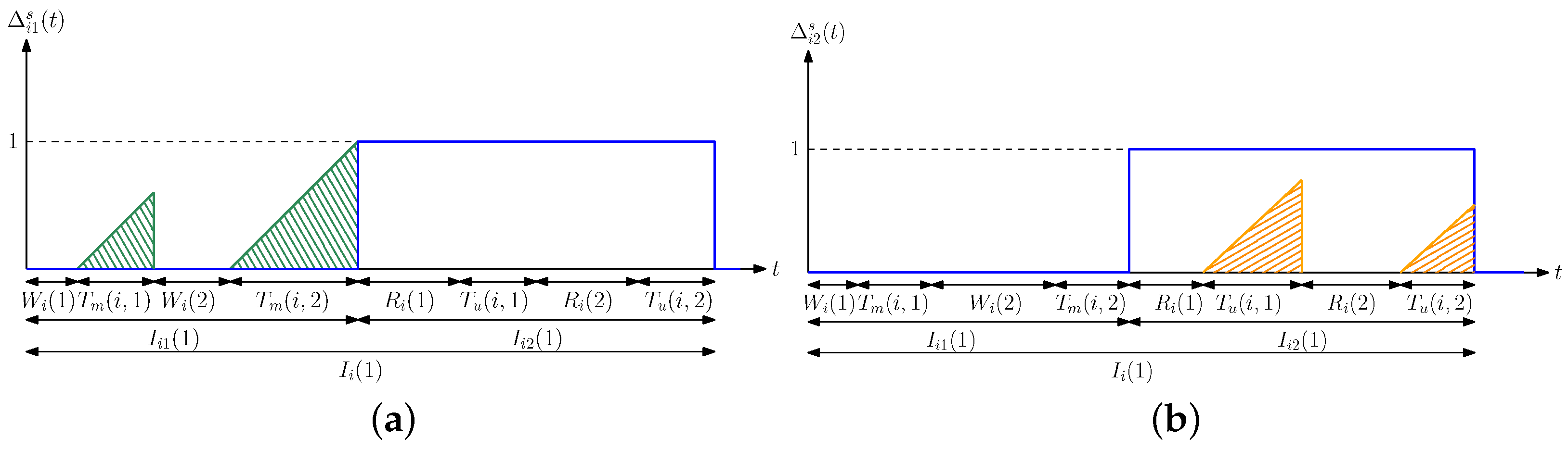
2. System Model
3. Average Difference Analysis
4. Optimization of Average Difference
5. Average Difference for the Case with Erroneous Test Measurements
5.1. An Alternative Method to Characterize Average Difference
5.2. Average Difference with Erroneous Test Measurements
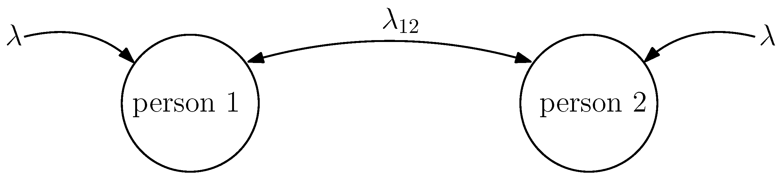
6. Average Estimation Error with Dependent Infection Rates
7. Age of Incorrect Information Based Error Metric
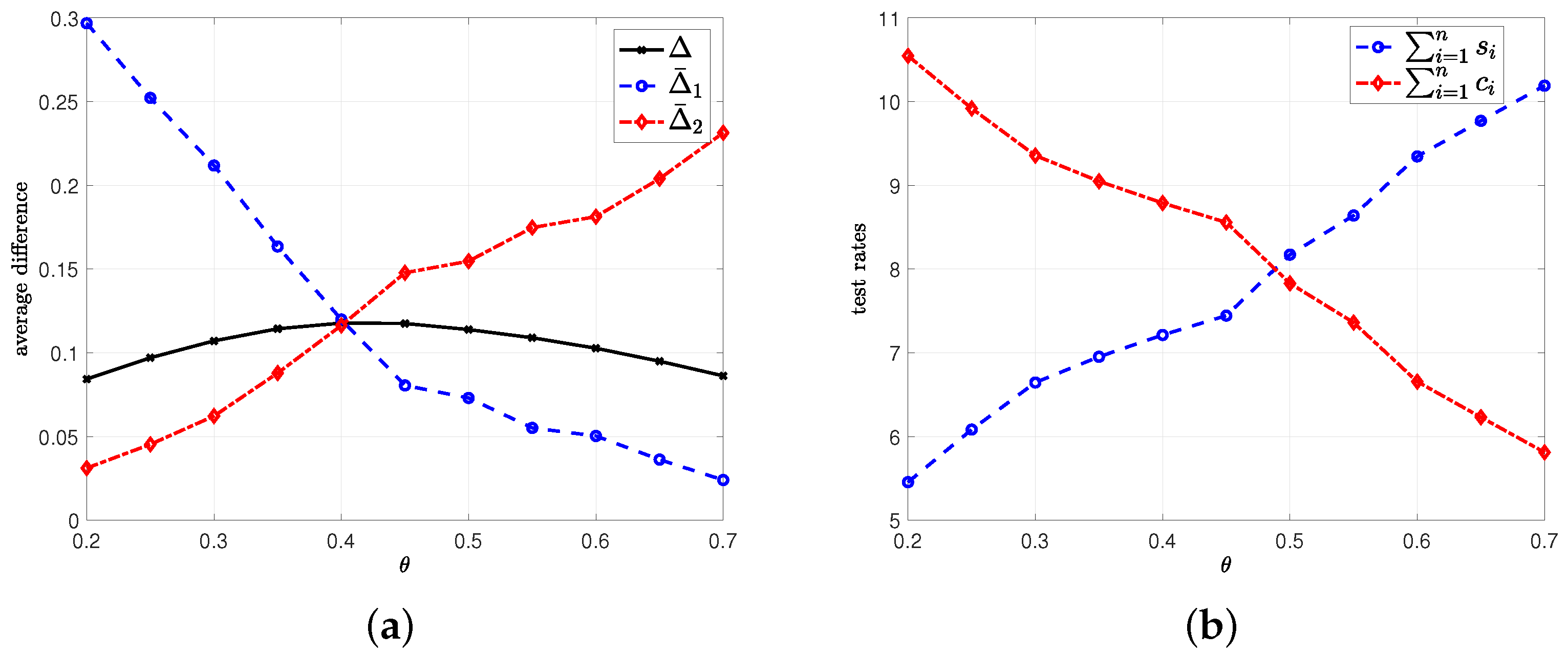
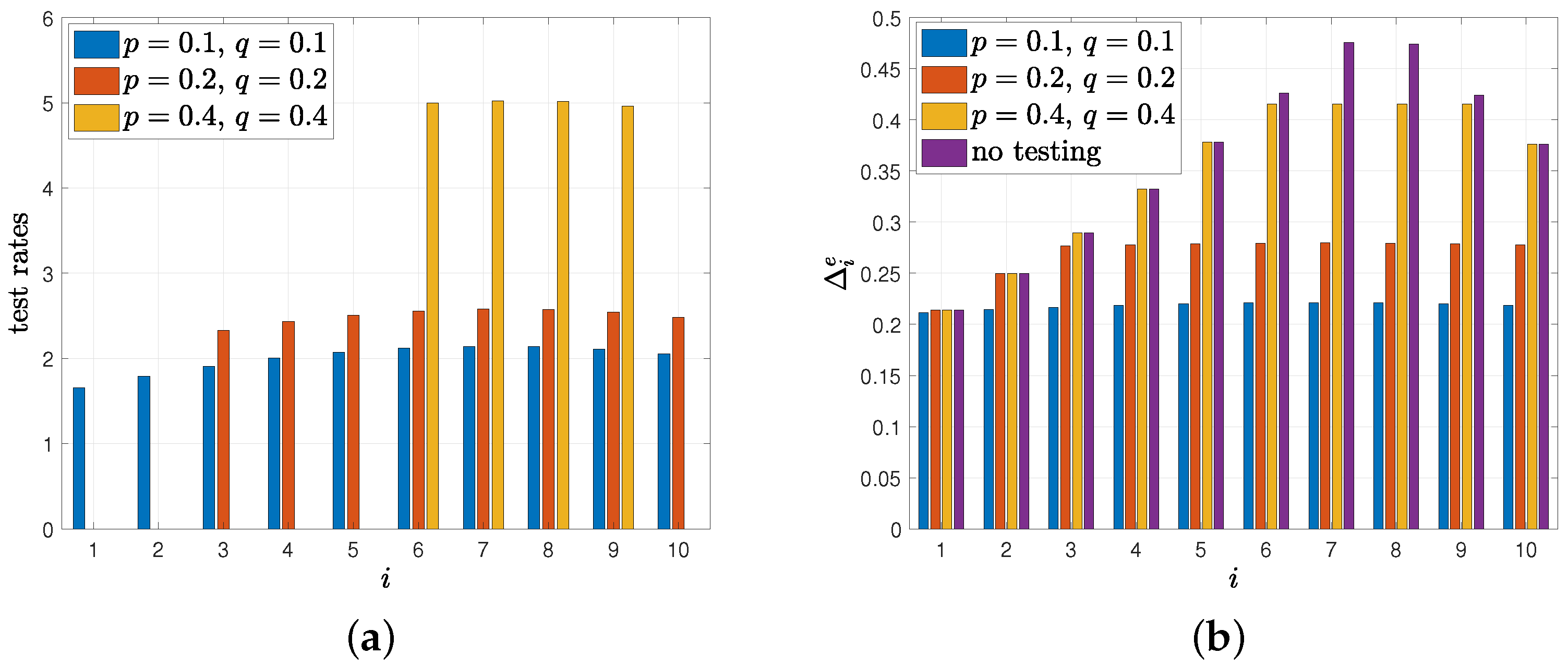
8. Numerical Results
9. Conclusions and Discussion
Author Contributions
Funding
Data Availability Statement
Conflicts of Interest
References
- Kaul, S.K.; Yates, R.D.; Gruteser, M. Real-time status: How often should one update? In Proceedings of the 2012 Proceedings IEEE INFOCOM, Orlando, FL, USA, 25–30 March 2012. [Google Scholar]
- Kadota, I.; Sinha, A.; Uysal-Biyikoglu, E.; Singh, R.; Modiano, E. Scheduling policies for minimizing age of information in broadcast wireless networks. IEEE/ACM Trans. Netw. 2018, 26, 2637–2650. [Google Scholar] [CrossRef] [Green Version]
- Kam, C.; Kompella, S.; Nguyen, G.D.; Wieselthier, J.E.; Ephremides, A. Age of information with a packet deadline. In Proceedings of the 2016 IEEE International Symposium on Information Theory (ISIT), Barcelona, Spain, 10–15 July 2016. [Google Scholar]
- Sun, Y.; Uysal-Biyikoglu, E.; Yates, R.D.; Koksal, C.E.; Shroff, N.B. Update or wait: How to keep your data fresh. IEEE Trans. Inf. Theory 2017, 63, 7492–7508. [Google Scholar] [CrossRef]
- Najm, E.; Telatar, E. Status updates in a multi-stream M/G/1/1 preemptive queue. In Proceedings of the IEEE Infocom 2018-IEEE Conference On Computer Communications Workshops (Infocom Wkshps), Honolulu, HI, USA, 15–19 April 2018. [Google Scholar]
- Soysal, A.; Ulukus, S. Age of information in G/G/1/1 systems: Age expressions, bounds, special cases, and optimization. IEEE Trans. Inf. Theory 2021, 67, 7477–7489. [Google Scholar] [CrossRef]
- Buyukates, B.; Ulukus, S. Age of information with Gilbert-Elliot servers and samplers. arXiv 2020, arXiv:2002.05711. [Google Scholar]
- Yates, R.D. The age of information in networks: Moments, distributions, and sampling. IEEE Trans. Inf. Theory 2020, 66, 5712–5728. [Google Scholar] [CrossRef]
- Talak, R.; Karaman, S.; Modiano, E. Minimizing age-of-information in multi-hop wireless networks. In Proceedings of the 2017 55th Annual Allerton Conference on Communication, Control, and Computing (Allerton), Monticello, IL, USA, 3–6 October 2017. [Google Scholar]
- Tripathi, V.; Moharir, S. Age of information in multi-source systems. In Proceedings of the GLOBECOM 2017-2017 IEEE Global Communications Conference, Centre, Singapore, 4–8 December 2017. [Google Scholar]
- Bedewy, A.M.; Sun, Y.; Shroff, N.B. The age of information in multihop networks. IEEE/ACM Trans. Netw. 2019, 27, 1248–1257. [Google Scholar] [CrossRef] [Green Version]
- Zhong, J.; Yates, R.D.; Soljanin, E. Multicast with prioritized delivery: How fresh is your data? In Proceedings of the 2018 IEEE 19th International Workshop on Signal Processing Advances in Wireless Communications (SPAWC), Kalamata, Greece, 25–28 June 2018. [Google Scholar]
- Buyukates, B.; Soysal, A.; Ulukus, S. Age of information in two-hop multicast networks. In Proceedings of the 2018 52nd Asilomar Conference on Signals, Systems, and Computers, Pacific Grove, CA, USA, 28–31 October 2018. [Google Scholar]
- Buyukates, B.; Soysal, A.; Ulukus, S. Age of information in multihop multicast networks. J. Commun. Netw. 2019, 21, 256–267. [Google Scholar] [CrossRef] [Green Version]
- Buyukates, B.; Soysal, A.; Ulukus, S. Age of information in multicast networks with multiple update streams. In Proceedings of the 2019 53rd Asilomar Conference on Signals, Systems, and Computers, Pacific Grove, CA, USA, 3–6 November 2019. [Google Scholar]
- Krishnan, K.S.A.; Sharma, V. Minimizing age of information in a multihop wireless network. In Proceedings of the ICC 2020-2020 IEEE International Conference on Communications, Dublin, Ireland, 7–11 June 2020. [Google Scholar]
- Farazi, S.; Klein, A.G.; Brown, D.R., III. Fundamental bounds on the age of information in multi-hop global status update networks. J. Commun. Netw. 2019, 21, 268–279. [Google Scholar] [CrossRef]
- Ioannidis, S.; Chaintreau, A.; Massoulie, L. Optimal and scalable distribution of content updates over a mobile social network. In Proceedings of the IEEE Infocom, Rio De Janeiro, Brazil, 24 April 2009. [Google Scholar]
- Wang, M.; Chen, W.; Ephremides, A. Reconstruction of counting process in real-time: The freshness of information through queues. In Proceedings of the ICC 2019-2019 IEEE International Conference on Communications (ICC), Shanghai, China, 20–24 May 2019. [Google Scholar]
- Sun, Y.; Polyanskiy, Y.; Uysal-Biyikoglu, E. Remote estimation of the Wiener process over a channel with random delay. In Proceedings of the 2017 IEEE International Symposium on Information Theory (ISIT), Aachen, Germany, 25–30 June 2017. [Google Scholar]
- Sun, Y.; Cyr, B. Information aging through queues: A mutual information perspective. In Proceedings of the 2018 IEEE 19th International Workshop on Signal Processing Advances in Wireless Communications (SPAWC), Kalamata, Greece, 25–28 June 2018. [Google Scholar]
- Chakravorty, J.; Mahajan, A. Remote estimation over a packet-drop channel with Markovian state. IEEE Trans. Autom. Control 2020, 65, 2016–2031. [Google Scholar] [CrossRef] [Green Version]
- Kam, C.; Kompella, S.; Ephremides, A. Age of incorrect information for remote estimation of a binary Markov source. In Proceedings of the IEEE INFOCOM 2020-IEEE Conference on Computer Communications Workshops (INFOCOM WKSHPS), Toronto, ON, Canada, 6–9 July 2020. [Google Scholar]
- Arafa, A.; Banawan, K.; Seddik, K.G.; Poor, H.V. Sample, quantize and encode: Timely estimation over noisy channels. IEEE Trans. Commun. 2021, 69, 6485–6499. [Google Scholar] [CrossRef]
- Bastopcu, M.; Ulukus, S. Who should Google Scholar update more often? In Proceedings of the IEEE INFOCOM 2020-IEEE Conference on Computer Communications Workshops (INFOCOM WKSHPS), Toronto, ON, Canada, 6–9 July 2020. [Google Scholar]
- Bacinoglu, B.T.; Sun, Y.; Uysal-Biyikoglu, E.; Mutlu, V. Achieving the age-energy trade-off with a finite-battery energy harvesting source. In Proceedings of the 2018 IEEE International Symposium on Information Theory (ISIT), Vail, CO, USA, 17–22 June 2018. [Google Scholar]
- Baknina, A.; Ozel, O.; Yang, J.; Ulukus, S.; Yener, A. Sending information through status updates. In Proceedings of the 2018 IEEE International Symposium on Information Theory (ISIT), Vail, CO, USA, 17–22 June 2018. [Google Scholar]
- Baknina, A.; Ulukus, S. Coded status updates in an energy harvesting erasure channel. In Proceedings of the 2018 52nd Annual Conference on Information Sciences and Systems (CISS), Princeton, NJ, USA, 21–23 March 2018. [Google Scholar]
- Wu, X.; Yang, J.; Wu, J. Optimal status update for age of information minimization with an energy harvesting source. IEEE Trans. Green Commun. Netw. 2018, 2, 193–204. [Google Scholar] [CrossRef]
- Feng, S.; Yang, J. Optimal status updating for an energy harvesting sensor with a noisy channel. In Proceedings of the IEEE INFOCOM 2018-IEEE Conference on Computer Communications Workshops (INFOCOM WKSHPS), Honolulu, HI, USA, 15–19 April 2018. [Google Scholar]
- Feng, S.; Yang, J. Minimizing age of information for an energy harvesting source with updating failures. In Proceedings of the 2018 IEEE International Symposium on Information Theory (ISIT), Vail, CO, USA, 17–22 June 2018. [Google Scholar]
- Arafa, A.; Yang, J.; Ulukus, S.; Poor, H.V. Age-minimal online policies for energy harvesting sensors with incremental battery recharges. In Proceedings of the 2018 Information Theory and Applications Workshop (ITA), San Diego, CA, USA, 11–16 February 2018. [Google Scholar]
- Arafa, A.; Yang, J.; Ulukus, S. Age-minimal online policies for energy harvesting sensors with random battery recharges. In Proceedings of the 2018 IEEE international conference on communications (ICC), Kansas City, MO, USA, 20–24 May 2018. [Google Scholar]
- Arafa, A.; Yang, J.; Ulukus, S.; Poor, H.V. Age-minimal transmission for energy harvesting sensors with finite batteries: Online policies. IEEE Trans. Inf. Theory 2020, 66, 534–556. [Google Scholar] [CrossRef] [Green Version]
- Arafa, A.; Yang, J.; Ulukus, S.; Poor, H.V. Online timely status updates with erasures for energy harvesting sensors. In Proceedings of the 2018 56th Annual Allerton Conference on Communication, Control, and Computing (Allerton), Monticello, IL, USA, 2–5 October 2018. [Google Scholar]
- Arafa, A.; Yang, J.; Ulukus, S.; Poor, H.V. Using erasure feedback for online timely updating with an energy harvesting sensor. In Proceedings of the 2019 IEEE International Symposium on Information Theory (ISIT), Paris, France, 7–12 July 2019. [Google Scholar]
- Arafa, A.; Yang, J.; Ulukus, S.; Poor, H.V. Timely status updating over erasure channels using an energy harvesting sensor: Single and multiple sources. IEEE Trans. Green Commun. Netw. 2022, 6, 6–19. [Google Scholar] [CrossRef]
- Farazi, S.; Klein, A.G.; Brown, D.R., III. Average age of information for status update systems with an energy harvesting server. In Proceedings of the IEEE INFOCOM 2018-IEEE Conference on Computer Communications Workshops (INFOCOM WKSHPS), Honolulu, HI, USA, 15–19 April 2018. [Google Scholar]
- Leng, S.; Yener, A. Age of information minimization for an energy harvesting cognitive radio. IEEE Trans. Cogn. Commun. Netw. 2019, 5, 427–439. [Google Scholar] [CrossRef]
- Chen, Z.; Pappas, N.; Bjornson, E.; Larsson, E.G. Age of information in a multiple access channel with heterogeneous traffic and an energy harvesting node. In Proceedings of the IEEE INFOCOM 2019-IEEE Conference on Computer Communications Workshops (INFOCOM WKSHPS), Paris, France, 29 April–2 May 2019. [Google Scholar]
- Bhat, R.V.; Vaze, R.; Motani, M. Throughput maximization with an average age of information constraint in fading channels. IEEE Trans. Wirel. Commun. 2021, 20, 481–494. [Google Scholar] [CrossRef]
- Ostman, J.; Devassy, R.; Durisi, G.; Uysal, E. Peak-age violation guarantees for the transmission of short packets over fading channels. In Proceedings of the IEEE INFOCOM 2019-IEEE Conference on Computer Communications Workshops (INFOCOM WKSHPS), Paris, France, 29 April–2 May 2019. [Google Scholar]
- Bastopcu, M.; Ulukus, S. Age of information with soft updates. In Proceedings of the 2018 56th Annual Allerton Conference on Communication, Control, and Computing (Allerton), Monticello, IL, USA, 2–5 October 2018. [Google Scholar]
- Bastopcu, M.; Ulukus, S. Minimizing age of information with soft updates. J. Commun. Netw. 2019, 21, 233–243. [Google Scholar] [CrossRef] [Green Version]
- Buyukates, B.; Soysal, A.; Ulukus, S. Age of information scaling in large networks. In Proceedings of the 2019 IEEE Global Communications Conference (GLOBECOM), Waikoloa, HI, USA, 9–13 December 2019. [Google Scholar]
- Buyukates, B.; Soysal, A.; Ulukus, S. Age of information scaling in large networks with hierarchical cooperation. In Proceedings of the 2019 IEEE Global Communications Conference (GLOBECOM), Waikoloa, HI, USA, 9–13 December 2019. [Google Scholar]
- Buyukates, B.; Soysal, A.; Ulukus, S. Scaling laws for age of information in wireless networks. IEEE Trans. Wirel. Commun. 2021, 20, 2413–2427. [Google Scholar] [CrossRef]
- Zhong, J.; Yates, R.D.; Soljanin, E. Minimizing content staleness in dynamo-style replicated storage systems. In Proceedings of the IEEE INFOCOM 2018-IEEE Conference on Computer Communications Workshops (INFOCOM WKSHPS), Honolulu, HI, USA, 15–19 April 2018. [Google Scholar]
- Rajaraman, N.; Vaze, R.; Reddy, G. Not just age but age and quality of information. IEEE J. Sel. Areas Commun. 2021, 39, 1325–1338. [Google Scholar] [CrossRef]
- Liu, Z.; Ji, B. Towards the tradeoff between service performance and information freshness. In Proceedings of the ICC 2019-2019 IEEE International Conference on Communications (ICC), Shanghai, China, 20–24 May 2019. [Google Scholar]
- Maatouk, A.; Assaad, M.; Ephremides, A. The age of incorrect information: An enabler of semantics-empowered communication. arXiv 2020, arXiv:2012.13214. [Google Scholar]
- Uysal, E.; Kaya, O.; Ephremides, A.; Gross, J.; Codreanu, M.; Popovski, P.; Johansson, K.H. Semantic communications in networked systems. arXiv 2021, arXiv:2103.05391. [Google Scholar]
- Ayan, O.; Vilgelm, M.; Klügel, M.; Hirche, S.; Kellerer, W. Age-of-information vs. value-of-information scheduling for cellular networked control systems. In Proceedings of the 10th ACM/IEEE International Conference on Cyber-Physical Systems, Montreal, QC, Canada, 16–18 April 2019. [Google Scholar]
- Bastopcu, M.; Ulukus, S. Timely group updating. In Proceedings of the 2021 55th Annual Conference on Information Sciences and Systems (CISS), Baltimore, MD, USA, 24–26 March 2021. [Google Scholar]
- Banerjee, S.; Bhattacharjee, R.; Sinha, A. Fundamental limits of age-of-information in stationary and non-stationary environments. In Proceedings of the 2020 IEEE International Symposium on Information Theory (ISIT), Los Angeles, CA, USA, 21–26 June 2020. [Google Scholar]
- Zhong, J.; Yates, R.D. Timeliness in lossless block coding. In Proceedings of the 2016 Data Compression Conference (DCC), Snowbird, UT, USA, 29 March–1 April 2016. [Google Scholar]
- Zhong, J.; Yates, R.D.; Soljanin, E. Timely lossless source coding for randomly arriving symbols. In Proceedings of the 2018 IEEE Information Theory Workshop (ITW), Guangzhou, China, 25–29 November 2018. [Google Scholar]
- Mayekar, P.; Parag, P.; Tyagi, H. Optimal lossless source codes for timely updates. In Proceedings of the 2018 IEEE International Symposium on Information Theory (ISIT), Vail, CO, USA, 17–22 June 2018. [Google Scholar]
- Mayekar, P.; Parag, P.; Tyagi, H. Optimal source codes for timely updates. IEEE Trans. Inf. Theory 2020, 66, 3714–3731. [Google Scholar] [CrossRef] [Green Version]
- Bastopcu, M.; Buyukates, B.; Ulukus, S. Optimal selective encoding for timely updates. In Proceedings of the 2020 54th Annual Conference on Information Sciences and Systems (CISS), Princeton, NJ, USA, 18–20 March 2020. [Google Scholar]
- Buyukates, B.; Bastopcu, M.; Ulukus, S. Optimal selective encoding for timely updates with empty symbol. In Proceedings of the 2020 IEEE International Symposium on Information Theory (ISIT), Los Angeles, CA, USA, 21–26 June 2020. [Google Scholar]
- Bastopcu, M.; Buyukates, B.; Ulukus, S. Selective encoding policies for maximizing information freshness. IEEE Trans. Commun. 2021, 69, 5714–5726. [Google Scholar] [CrossRef]
- Ramirez, D.; Erkip, E.; Poor, H.V. Age of information with finite horizon and partial updates. In Proceedings of the ICASSP 2020-2020 IEEE International Conference on Acoustics, Speech and Signal Processing (ICASSP), Barcelona, Spain, 4–8 May 2020. [Google Scholar]
- Arafa, A.; Banawan, K.; Seddik, K.G.; Poor, H.V. On timely channel coding with hybrid ARQ. In Proceedings of the 2019 IEEE Global Communications Conference (GLOBECOM), Big Island, HI, USA, 9–13 December 2019. [Google Scholar]
- Arafa, A.; Wesel, R.D. Timely transmissions using optimized variable length coding. In Proceedings of the IEEE INFOCOM 2021-IEEE Conference on Computer Communications Workshops (INFOCOM WKSHPS), Vancouver, BC, Canada, 10–13 May 2021. [Google Scholar]
- Bastopcu, M.; Ulukus, S. Partial updates: Losing information for freshness. In Proceedings of the 2020 IEEE International Symposium on Information Theory (ISIT), Los Angeles, CA, USA, 21–26 June 2020. [Google Scholar]
- Abd-Elmagid, M.A.; Dhillon, H.S. Average peak age-of-information minimization in UAV-assisted IoT networks. IEEE Trans. Veh. Technol. 2019, 68, 2003–2008. [Google Scholar] [CrossRef] [Green Version]
- Liu, J.; Wang, X.; Dai, H. Age-optimal trajectory planning for UAV-assisted data collection. In Proceedings of the IEEE INFOCOM 2018-IEEE Conference on Computer Communications Workshops (INFOCOM WKSHPS), Honolulu, HI, USA, 15–19 April 2018. [Google Scholar]
- Abd-Elmagid, M.A.; Pappas, N.; Dhillon, H.S. On the role of age of information in the internet of things. IEEE Commun. Mag. 2019, 57, 72–77. [Google Scholar] [CrossRef] [Green Version]
- Alabbasi, A.; Aggarwal, V. Joint information freshness and completion time optimization for vehicular networks. IEEE Trans. Serv. Comput. 2020, 15, 1–14. [Google Scholar] [CrossRef] [Green Version]
- Gao, W.; Cao, G.; Srivatsa, M.; Iyengar, A. Distributed maintenance of cache freshness in opportunistic mobile networks. In Proceedings of the 2012 IEEE 32nd International Conference on Distributed Computing Systems, Macau, China, 18–21 June 2012. [Google Scholar]
- Yates, R.D.; Ciblat, P.; Yener, A.; Wigger, M. Age-optimal constrained cache updating. In Proceedings of the 2017 IEEE International Symposium on Information Theory (ISIT), Aachen, Germany, 25–30 June 2017. [Google Scholar]
- Kam, C.; Kompella, S.; Nguyen, G.D.; Wieselthier, J.E.; Ephremides, A. Information freshness and popularity in mobile caching. In Proceedings of the 2017 IEEE International Symposium on Information Theory (ISIT), Aachen, Germany, 25–30 June 2017. [Google Scholar]
- Zhang, S.; Li, J.; Luo, H.; Gao, J.; Zhao, L.; Shen, X.S. Towards fresh and low-latency content delivery in vehicular networks: An edge caching aspect. In Proceedings of the 2018 10th International Conference on Wireless Communications and Signal Processing (WCSP), Hangzhou, China, 18–20 October 2018. [Google Scholar]
- Tang, H.; Ciblat, P.; Wang, J.; Wigger, M.; Yates, R. Age of information aware cache updating with file- and age-dependent update durations. In Proceedings of the 2020 18th International Symposium on Modeling and Optimization in Mobile, Ad Hoc, and Wireless Networks (WiOPT), Volos, Greece, 15–19 June 2020. [Google Scholar]
- Zhong, J.; Yates, R.D.; Soljanin, E. Two freshness metrics for local cache refresh. In Proceedings of the 2018 IEEE International Symposium on Information Theory (ISIT), Vail, CO, USA, 17–22 June 2018. [Google Scholar]
- Yang, L.; Zhong, Y.; Zheng, F.; Jin, S. Edge caching with real-time guarantees. arXiv 2019, arXiv:1912.11847. [Google Scholar]
- Bastopcu, M.; Ulukus, S. Maximizing information freshness in caching systems with limited cache storage capacity. In Proceedings of the 2020 54th Asilomar Conference on Signals, Systems, and Computers, Pacific Grove, CA, USA, 1–5 November 2020. [Google Scholar]
- Bastopcu, M.; Ulukus, S. Cache freshness in information updating systems. In Proceedings of the 2021 55th Annual Conference on Information Sciences and Systems (CISS), Baltimore, MD, USA, 24–26 March 2021. [Google Scholar]
- Bastopcu, M.; Ulukus, S. Information freshness in cache updating systems. IEEE Trans. Wirel. Commun. 2021, 20, 1861–1874. [Google Scholar] [CrossRef]
- Kaswan, P.; Bastopcu, M.; Ulukus, S. Freshness based cache updating in parallel relay networks. In Proceedings of the 2021 IEEE International Symposium on Information Theory (ISIT), Melbourne, Australia, 12–20 July 2021. [Google Scholar]
- Gu, Y.; Wang, Q.; Chen, H.; Li, Y.; Vucetic, B. Optimizing information freshness in two-hop status update systems under a resource constraint. IEEE J. Sel. Areas Commun. 2021, 39, 1380–1392. [Google Scholar] [CrossRef]
- Kuang, Q.; Gong, J.; Chen, X.; Ma, X. Age-of-information for computation-intensive messages in mobile edge computing. arXiv 2019, arXiv:1901.01854. [Google Scholar]
- Gong, J.; Kuang, Q.; Chen, X.; Ma, X. Reducing age-of-information for computation-intensive messages via packet replacement. In Proceedings of the 2019 11th International Conference on Wireless Communications and Signal Processing (WCSP), Xi’an, China, 23–25 October 2019. [Google Scholar]
- Zou, P.; Ozel, O.; Subramaniam, S. Trading off computation with transmission in status update systems. In Proceedings of the 2019 IEEE 30th Annual International Symposium on Personal, Indoor and Mobile Radio Communications (PIMRC), Istanbul, Turkey, 8–11 September 2019. [Google Scholar]
- Bastopcu, M.; Ulukus, S. Age of information for updates with distortion. In Proceedings of the 2019 IEEE Information Theory Workshop (ITW), Gotland, Sweden, 25–28 August 2019. [Google Scholar]
- Bastopcu, M.; Ulukus, S. Age of information for updates with distortion: Constant and age-dependent distortion constraints. IEEE/ACM Trans. Netw. 2021, 29, 2425–2438. [Google Scholar] [CrossRef]
- Buyukates, B.; Ulukus, S. Timely updates in distributed computation systems with stragglers. In Proceedings of the 2020 54th Asilomar Conference on Signals, Systems, and Computers, Pacific Grove, CA, USA, 1–5 November 2020. [Google Scholar]
- Buyukates, B.; Ulukus, S. Timely distributed computation with stragglers. IEEE Trans. Commun. 2020, 68, 5273–5282. [Google Scholar] [CrossRef]
- Zou, P.; Ozel, O.; Subramaniam, S. Optimizing information freshness through computation–transmission tradeoff and queue management in edge computing. IEEE/ACM Trans. Netw. 2021, 29, 949–963. [Google Scholar] [CrossRef]
- Buyukates, B.; Ulukus, S. Timely communication in federated learning. In Proceedings of the IEEE INFOCOM 2021-IEEE Conference on Computer Communications Workshops (INFOCOM WKSHPS), Vancouver, BC, Canada, 10–13 May 2021. [Google Scholar]
- Ozfatura, E.; Buyukates, B.; Gündüz, D.; Ulukus, S. Age-based coded computation for bias reduction in distributed learning. In Proceedings of the GLOBECOM 2020-2020 IEEE Global Communications Conference, Taipei, Taiwan, 7–11 December 2020. [Google Scholar]
- Ceran, E.T.; Gündüz, D.; György, A. A reinforcement learning approach to age of information in multi-user networks with HARQ. IEEE J. Sel. Areas Commun. 2021, 39, 1412–1426. [Google Scholar] [CrossRef]
- Yates, R.D. The age of gossip in networks. In Proceedings of the 2021 IEEE International Symposium on Information Theory (ISIT), Melbourne, Australia, 12–20 July 2021. [Google Scholar]
- Buyukates, B.; Bastopcu, M.; Ulukus, S. Age of gossip in networks with community structure. In Proceedings of the 2021 IEEE 22nd International Workshop on Signal Processing Advances in Wireless Communications (SPAWC), Lucca, Italy, 27–30 September 2021. [Google Scholar]
- Bastopcu, M.; Buyukates, B.; Ulukus, S. Gossiping with binary freshness metric. In Proceedings of the 2021 IEEE Globecom Workshops (GC Wkshps), Madrid, Spain, 7–11 December 2021. [Google Scholar]
- Kaswan, P.; Ulukus, S. Timely gossiping with file slicing and network coding. arXiv 2022, arXiv:2202.00649. [Google Scholar]
- Kosta, A.; Pappas, N.; Angelakis, V. Age of information: A new concept, metric, and tool. Found. Trends Netw. 2017, 12, 162–259. [Google Scholar] [CrossRef] [Green Version]
- Sun, Y.; Kadota, I.; Talak, R.; Modiano, E. Age of information: A new metric for information freshness. Synth. Lect. Commun. Netw. 2019, 12, 1–224. [Google Scholar] [CrossRef]
- Yates, R.D.; Sun, Y.; Brown, D.R., III; Kaul, S.K.; Modiano, E.; Ulukus, S. Age of information: An introduction and survey. IEEE J. Sel. Areas Commun. 2021, 39, 1183–1210. [Google Scholar] [CrossRef]
- Yun, J.; Joo, C.; Eryilmaz, A. Optimal real-time monitoring of an information source under communication costs. In Proceedings of the 2018 IEEE Conference on Decision and Control (CDC), Miami Beach, FL, USA, 17–19 December 2018. [Google Scholar]
- Maatouk, A.; Kriouile, S.; Assaad, M.; Ephremides, A. The age of incorrect information: A new performance metric for status updates. IEEE/ACM Trans. Netw. 2020, 28, 2215–2228. [Google Scholar] [CrossRef]
- Yates, R.D.; Goodman, D.J. Probability and Stochastic Processes; Wiley: Hoboken, NJ, USA, 2014. [Google Scholar]
- Boyd, S.P.; Vandenberghe, L. Convex Optimization; Cambridge University Press: Cambridge, UK, 2004. [Google Scholar]
- Bertsekas, D.P.; Tsitsiklis, J.N. Introduction to Probability; Athena Scientific: Belmont, MA, USA, 2008. [Google Scholar]
- Chen, Y.C.; Lu, P.E.; Chang, C.S.; Liu, T.H. A time-dependent SIR model for COVID-19 with undetectable infected persons. IEEE Trans. Netw. Sci. Eng. 2020, 7, 3279–3294. [Google Scholar] [CrossRef]
- Olmez, S.Y.; Mori, J.; Miehling, E.; Başar, T.; Smith, R.L.; West, M.; Mehta, P.G. A data-informed approach for analysis, validation, and identification of COVID-19 models. In Proceedings of the 2021 American Control Conference (ACC), New Orleans, LA, USA, 25–28 May 2021. [Google Scholar]


| Variables | Definition of the Variables |
|---|---|
| Section 2, Section 3 and Section 4 | |
| n | number of people in the population |
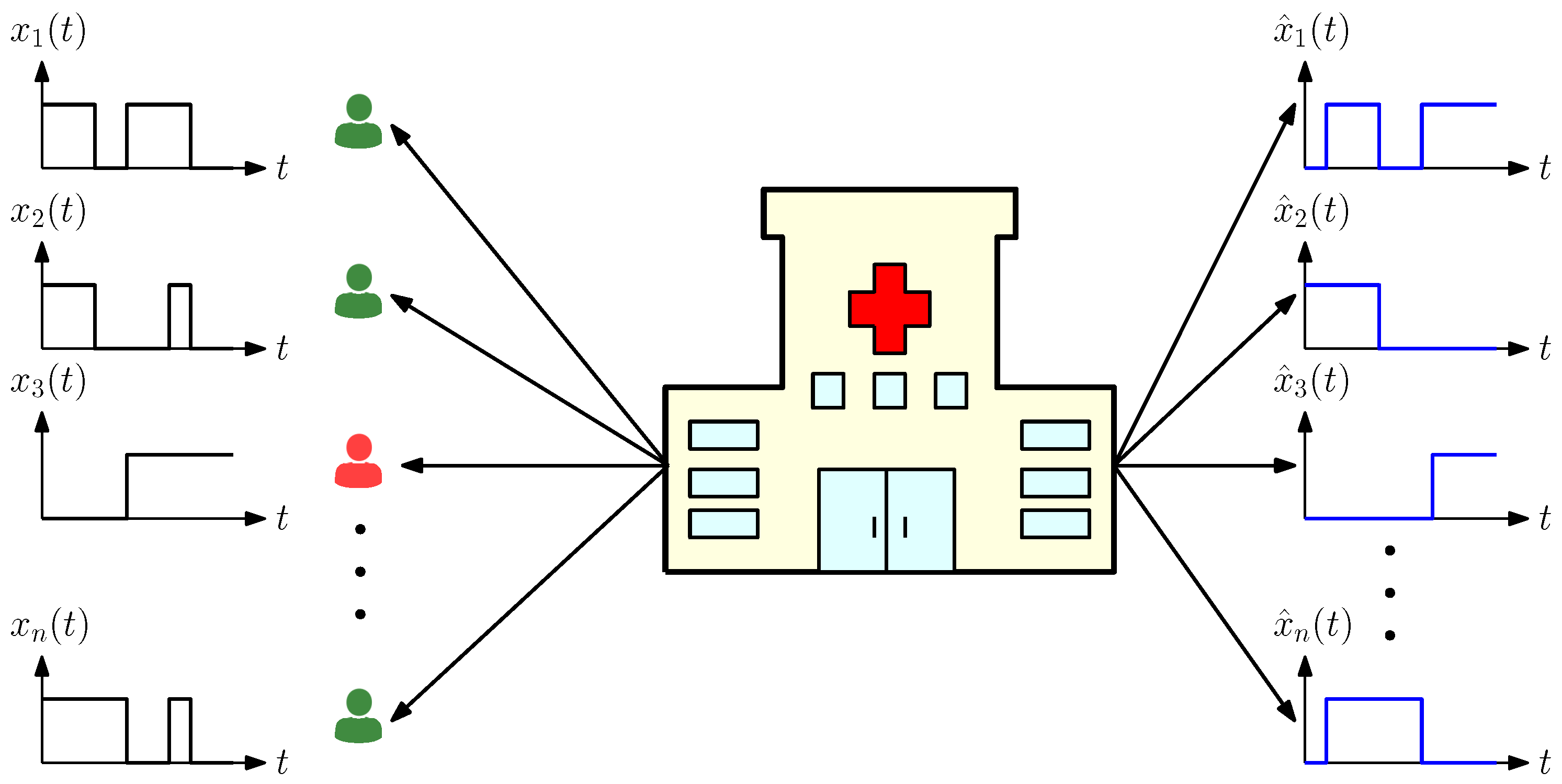
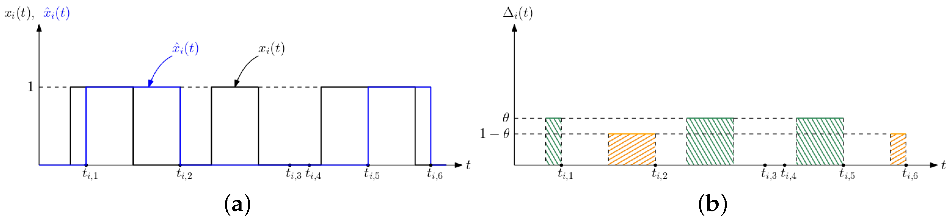
| infection status of the ith person at time t | |
| estimation of at the health care provider | |
| infection and recovery rates for the ith person | |
| , | test rates applied to the ith person when , and |
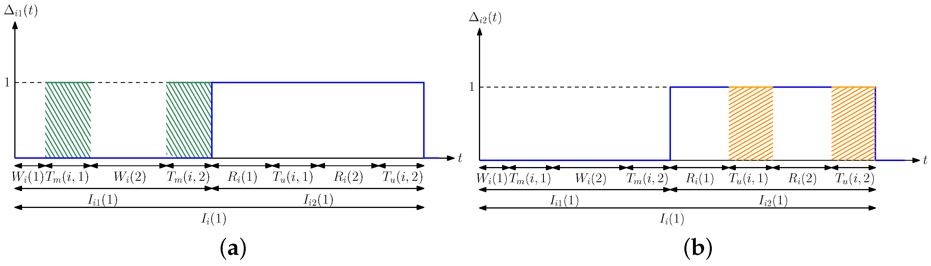
| total estimation error for the ith person at time t | |
| importance factor in | |
| the long-time weighted average for the ith person | |
| C | total test rate constraint |
| Section 5 | |
| the long-time average difference for the ith person with | |
| erroneous test measurements | |
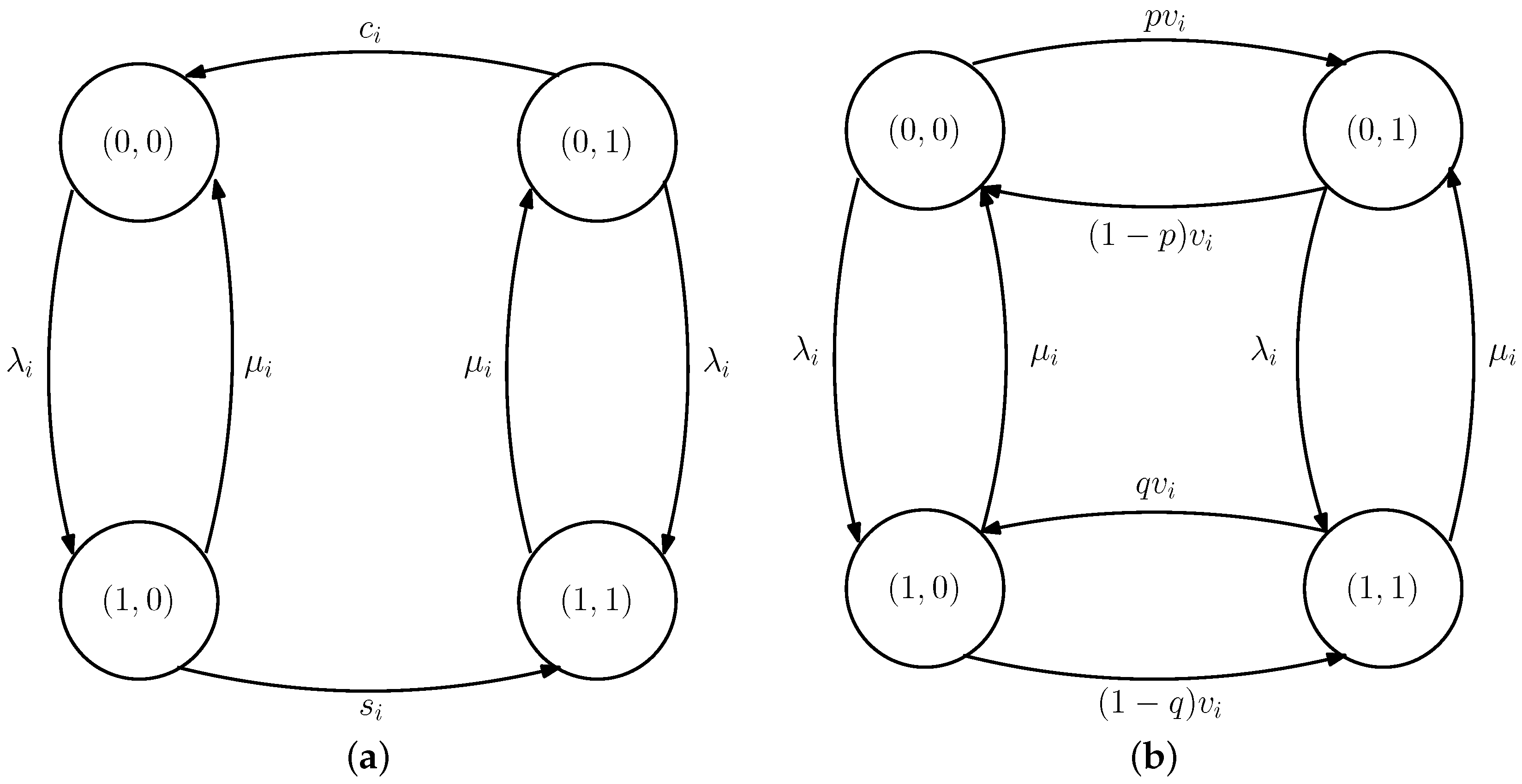
| q | false-negative testing probability with |
| p | false-positive testing probability with |
| test rate applied to the ith person with erroneous test measurements | |
| Section 6 | |
| individual infection and recovery rate of a person | |
| the rate of spreading the virus from an undetected infected person | |
| to a healthy person | |
| c, s | test rates applied to people when , and |
| the long-time average difference for the ith person with | |
| dependent infection rates | |
| Section 7 | |
| test rate applied to the ith person for AoII-based error metric | |
| the long-time average difference for the ith person with | |
| AoII-based error metric |
| ∖ | 0 | 1 |
|---|---|---|
| 0 | p | |
| 1 | q |
Publisher’s Note: MDPI stays neutral with regard to jurisdictional claims in published maps and institutional affiliations. |
© 2022 by the authors. Licensee MDPI, Basel, Switzerland. This article is an open access article distributed under the terms and conditions of the Creative Commons Attribution (CC BY) license (https://creativecommons.org/licenses/by/4.0/).
Share and Cite
Bastopcu, M.; Ulukus, S. Using Timeliness in Tracking Infections. Entropy 2022, 24, 779. https://doi.org/10.3390/e24060779
Bastopcu M, Ulukus S. Using Timeliness in Tracking Infections. Entropy. 2022; 24(6):779. https://doi.org/10.3390/e24060779
Chicago/Turabian StyleBastopcu, Melih, and Sennur Ulukus. 2022. "Using Timeliness in Tracking Infections" Entropy 24, no. 6: 779. https://doi.org/10.3390/e24060779
APA StyleBastopcu, M., & Ulukus, S. (2022). Using Timeliness in Tracking Infections. Entropy, 24(6), 779. https://doi.org/10.3390/e24060779