
Rolling Bearing Fault Diagnosis Using Multi-Sensor Data Fusion Based on 1D-CNN Model


Abstract
:1. Introduction
- (1)
- An improved SWD algorithm, namely BAS-SWD, is proposed. By adopting the BAS algorithm to obtain the optimal parameters of SWD, the OCs with more obvious fault information can be obtained.
- (2)
- Based on the model of VGG-16, the improved 1D-CNN model is proposed to extract the weak features in multi-sensor signals. Through the well-trained model, the features in the raw signals can be extracted, and the high accuracy of classification is verified by different datasets.
- (3)
- The feature fusion strategy is introduced, and the features extracted by different convolutional blocks in the 1D-CNN model are fused in the fusion layer. Based on feature fusion, the classification accuracy of the model is improved obviously.
2. Optimal Swarm Decomposition
2.1. The Beetle Antennae Search Optimization Algorithm
- (1)
- Initialize the initial position x0 and distance between two antennas of the beetle d0. Notably, d0 should be large enough to improve detection ability. Additionally, then define a vector x = {xi, I = 1, 2, ... L} to record beetle’s position during each iteration; L is the maximum number of iterations.
- (2)
- Defines the fitness function, fitness(·), to represent the odor concentration of food.
- (3)
- During each iteration, the direction of beetle’s antennae is initialized as a normalized random vector using Equation (1). Then, the coordinates of beetle’s two antennas can be calculated by Equation (2).where rand(·) is the random function, is the 1-norm of a vector, and x.i is the coordinate of beetle’s antenna at i-th iteration, xi is the position of beetle, and di is the distance between beetle’s antennas currently.
- (4)
- Calculate the value of fitness function with x.i and let the beetle take a step to the direction of the antenna, which has a smaller fitness value. After that, the position and distance between antennas and step length of beetle are updated using Equations (3)–(5).where sgn(·) is the sign function.
- (5)
- Check the iteration stop condition (i.e., i reaches the maximum number of iterations L) is met or not; if not, repeat step (3) to (4) until the iteration stop condition is satisfied.
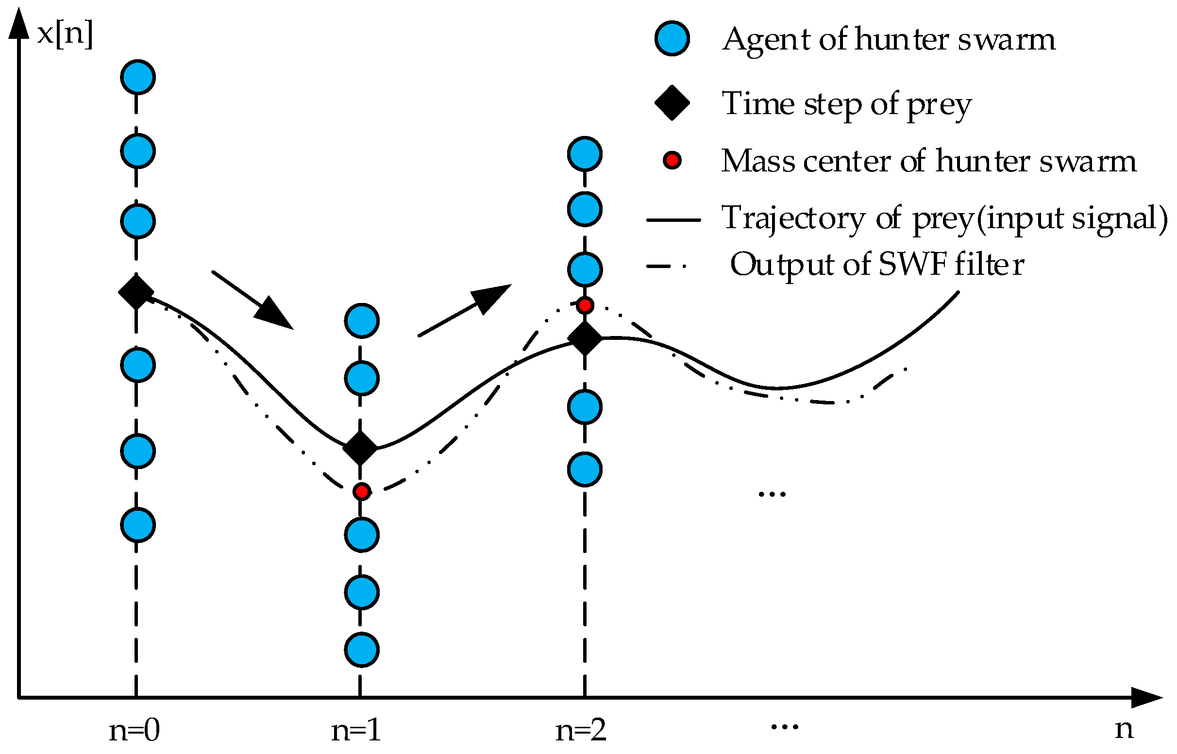
2.2. The Original Swarm Decomposition
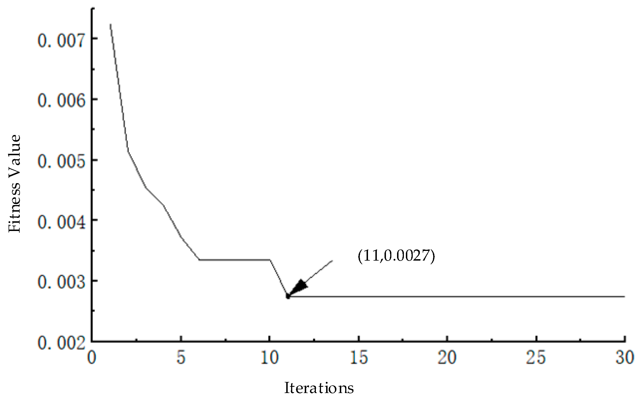
2.3. Improve of Swarm Decomposition
| Algorithm 1. BAS-SWD |
| Input: multi-component signal Output: Pωth, Tth |
| Initialize parameters of BAS: L, d0, δ0, n, Pωth, lb, Pωth_ub, Tth_lb, Tth_ub Definition of fitness function: fit(·) ← Equation (13) Initialize of variables: x0 Definition of list of best positons: best_p ← Array [] Definition of list of best values: best_v ← Array [] i ← 0 while i < L − 1 Calculate fitness value: fit ← fit(xi) Save the position: best_p[i] ← xi Save the fitness value: best_v[i] ← fit Calculate the head’s toward: ← Equation (1) Calculate the position of antennas: ← Equation (2) Update the positon of beetle: ← Equation (3) Update the position of antennas: ← Equation (4) Update the step length: ← Equation (5) i ← i + 1 end of while Search the positon of minimum fitness value: idx ← min-index(best_v) Return best_p[idx] |
3. One-Dimension Convolutional Neural Network
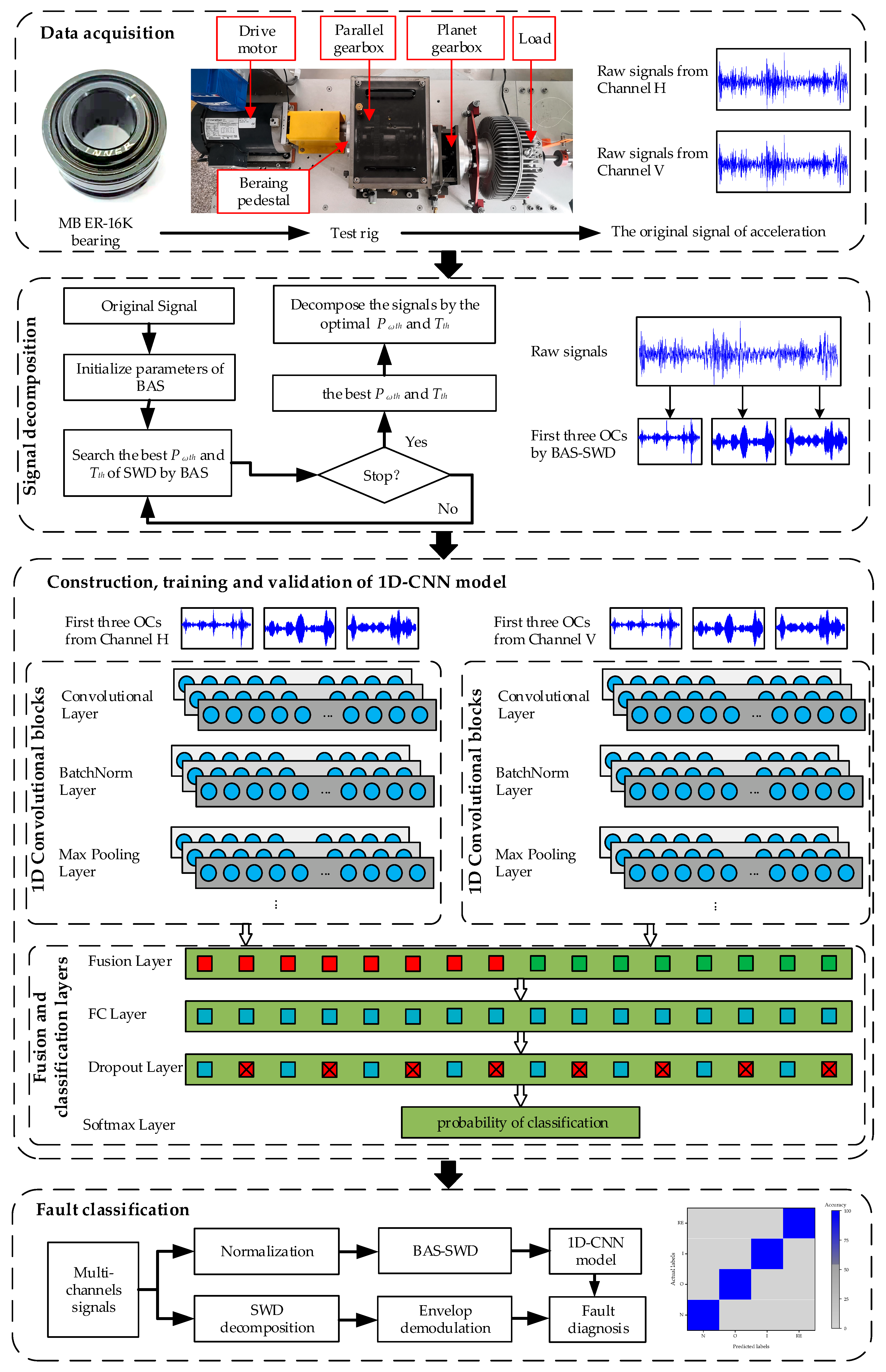
4. The Proposed Method
5. Experimental Validations
5.1. Data Information
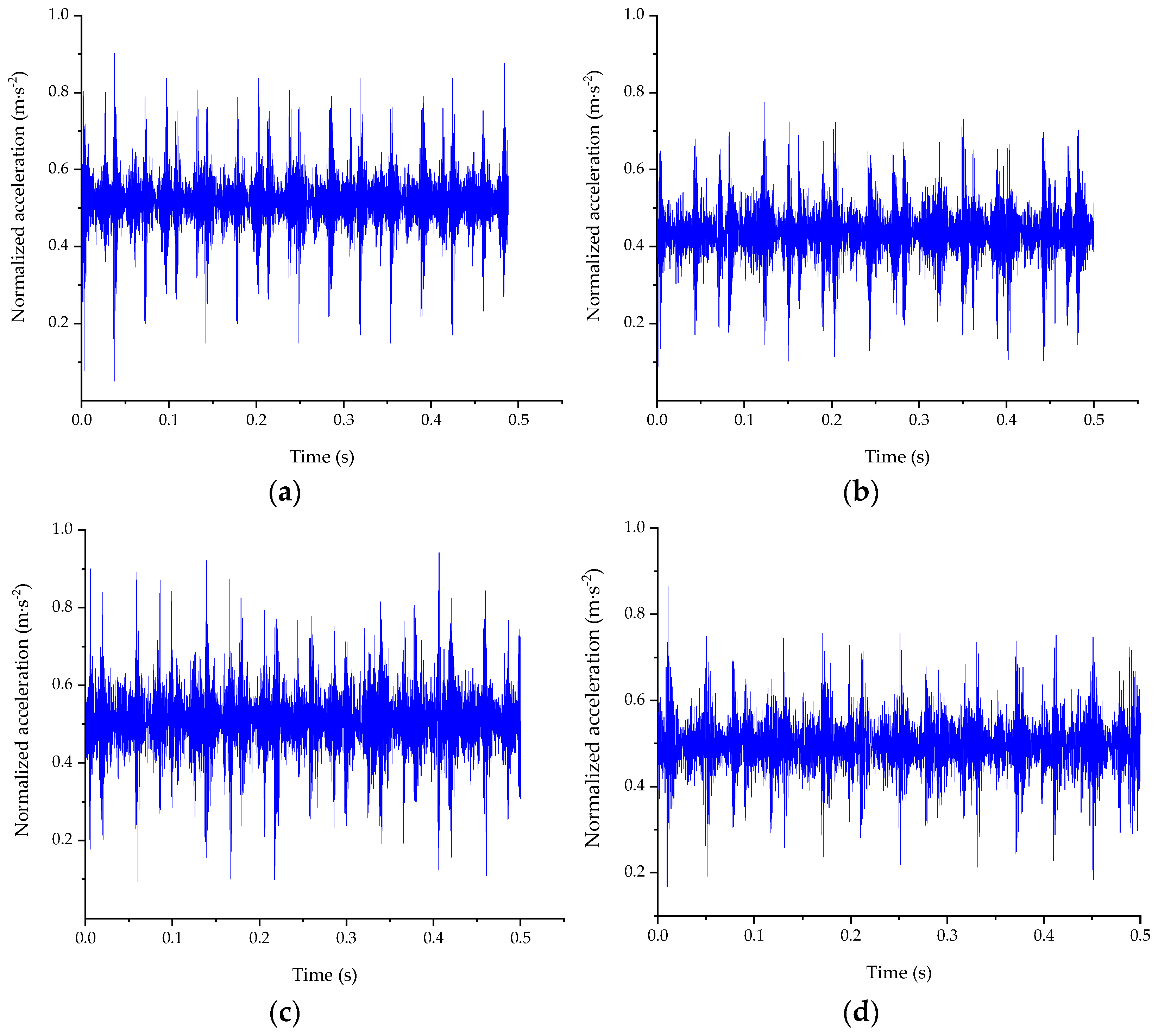
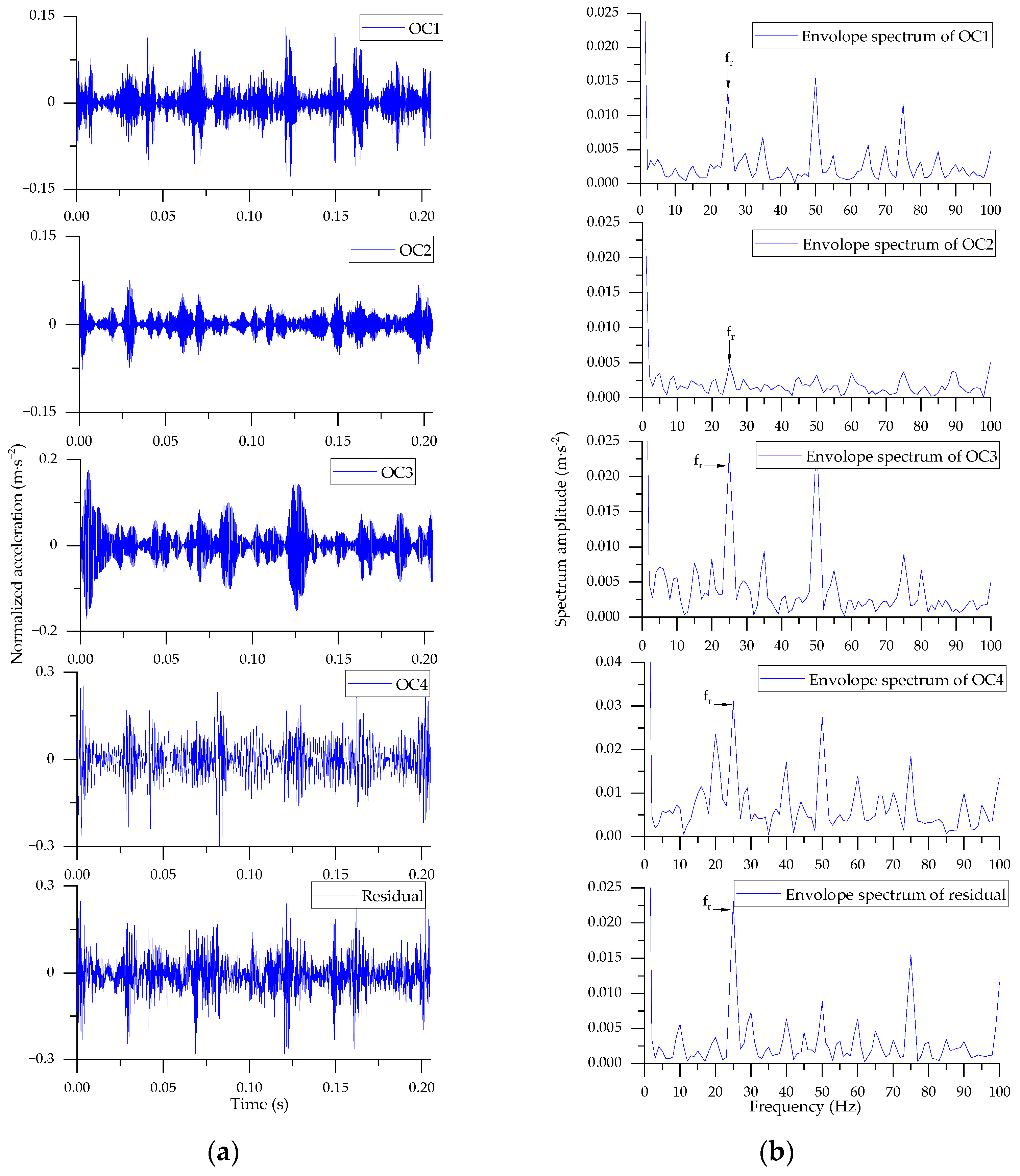
5.2. Preprocessing of Signals
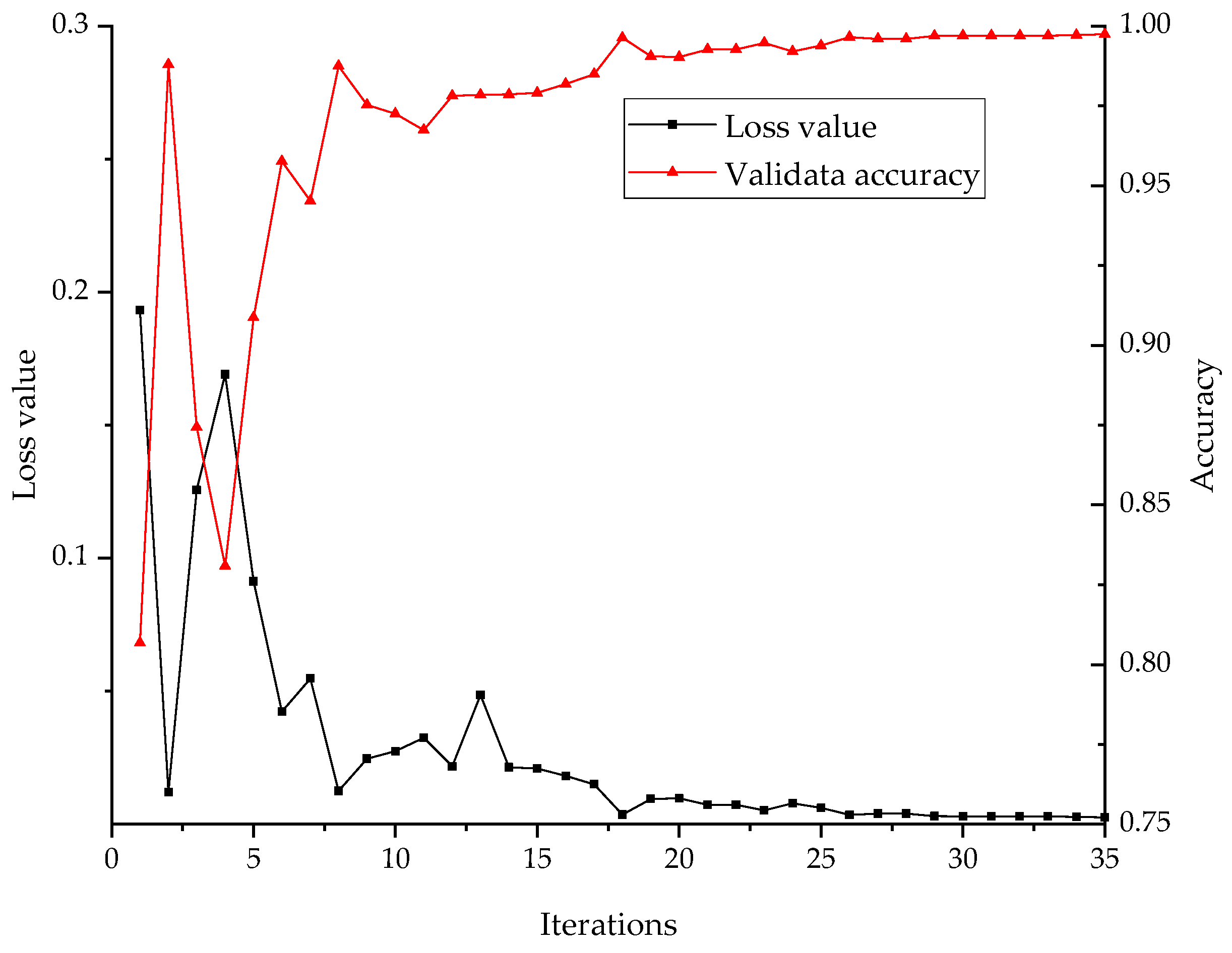
5.3. Construction of 1D-CNN Model
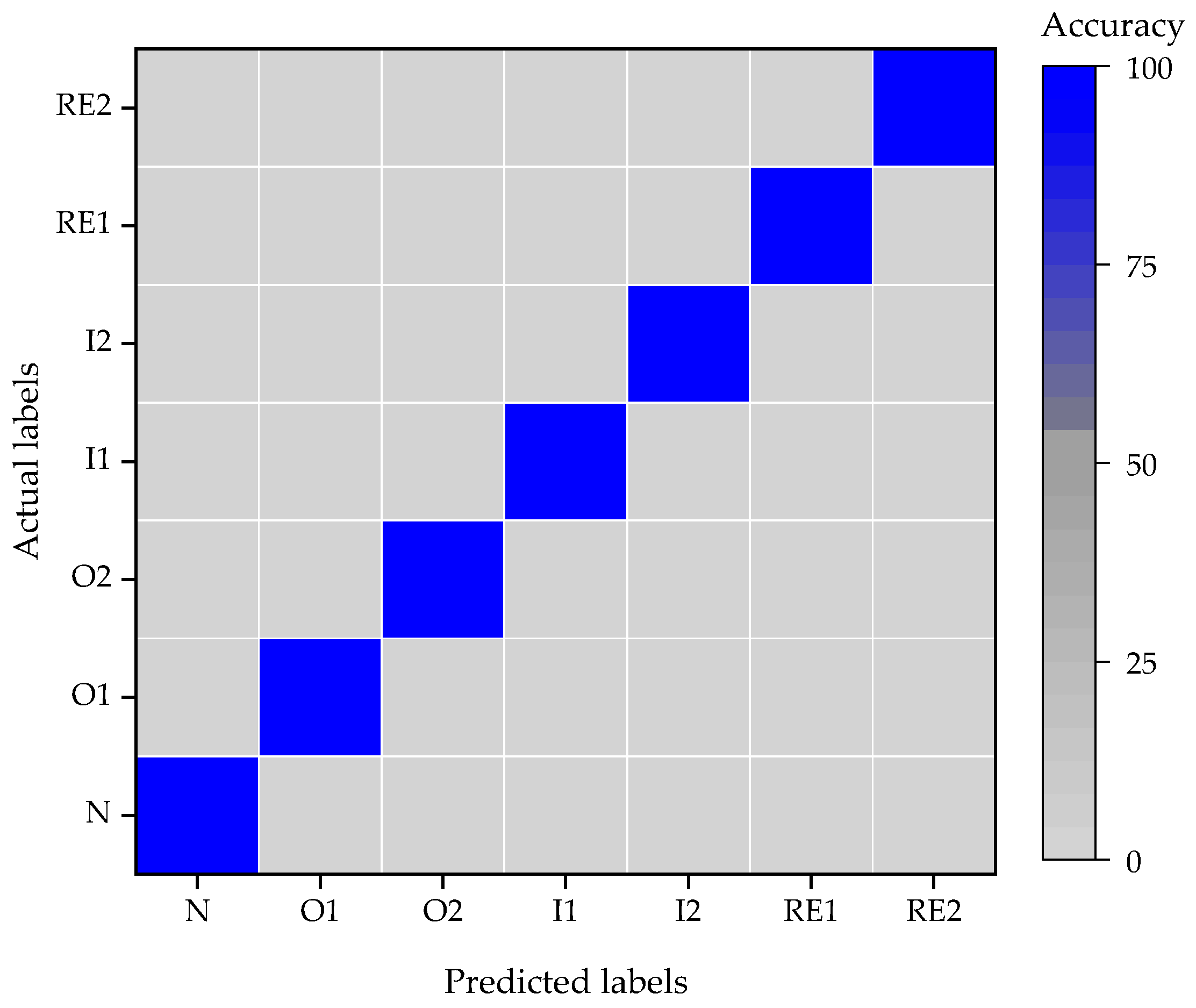
5.4. Case Study I
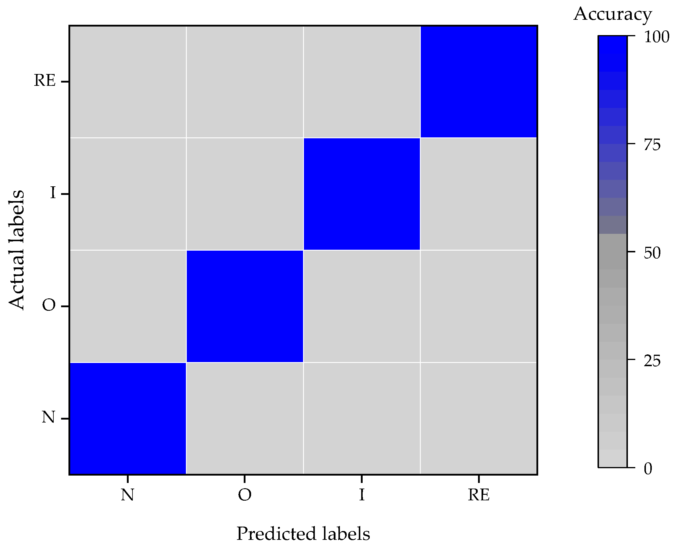
5.5. Case Study II
6. Conclusions
Author Contributions
Funding
Institutional Review Board Statement
Informed Consent Statement
Data Availability Statement
Conflicts of Interest
References
- Ma, J.; Li, Z.; Li, C.; Zhan, L.; Zhang, G. Rolling Bearing Fault Diagnosis Based on Refined Composite Multi-Scale Approximate Entropy and Optimized Probabilistic Neural Network. Entropy 2021, 23, 259. [Google Scholar] [CrossRef] [PubMed]
- Yan, X.; Xu, Y.; She, D.; Zhang, W. Reliable Fault Diagnosis of Bearings Using an Optimized Stacked Variational Denoising Auto-Encoder. Entropy 2022, 24, 36. [Google Scholar] [CrossRef] [PubMed]
- Luo, S.; Yang, W.; Luo, Y. Fault Diagnosis of a Rolling Bearing Based on Adaptive Sparest Narrow-Band Decomposition and Refined Composite Multiscale Dispersion Entropy. Entropy 2020, 22, 375. [Google Scholar] [CrossRef] [PubMed] [Green Version]
- Wang, H.; Sun, W.; He, L.; Zhou, J. Intelligent Fault Diagnosis Method for Gear Transmission Systems Based on Improved Multi-Scale Reverse Dispersion Entropy and Swarm Decomposition. IEEE Trans. Instrum. Meas. 2022, 71, 1–13. [Google Scholar] [CrossRef]
- Glowacz, A.; Glowacz, W.; Glowaz, Z.; Kozik, J. Early Fault Diagnosis of Bearing and Stator Faults of the Single-Phase Induction Motor Using Acoustic Signals. Measurement 2018, 113, 1–9. [Google Scholar] [CrossRef]
- Pang, B.; Nazari, M.; Tang, G. Recursive Variational Mode Extraction and Its Application in Rolling Bearing Fault Diagnosis. Mech. Syst. Signal Process. 2022, 165, 108321. [Google Scholar] [CrossRef]
- Huang, N.E.; Shen, Z.; Long, S.R.; Wu, M.C.; Shih, H.H.; Zheng, Q.; Yen, N.; Tung, C.C.; Liu, H.H. The Empirical Mode Decomposition and the Hilbert Spectrum for Nonlinear and Non-Stationary Time Series Analysis. Proc. Math. Phys. Eng. Sci. 1998, 454, 903–995. [Google Scholar] [CrossRef]
- Wu, Z.; Huang, N.E. Ensemble empirical mode decomposition: A noise-assisted data analysis method. Adv. Adapt. Data Anal. 2009, 1, 1–41. [Google Scholar] [CrossRef]
- Yeh, J.R.; Shieh, J.S.; Huang, N.E. Complementary Ensemble Empirical Mode Decomposition: A Novel Noise Enhanced Data Analysis Method. Adv. Adapt. Data Anal. 2010, 2, 135–156. [Google Scholar] [CrossRef]
- Yu, Y.; Li, W.; Sheng, D.; Chen, J. A Novel Sensor Fault Diagnosis Method Based on Modified Ensemble Empirical Mode Decomposition and Probabilistic Neural Network. Measurement 2015, 68, 328–336. [Google Scholar] [CrossRef]
- Torres, M.E.; Colominas, M.A.; Schlotthauer, G.; Flandrin, P. A Complete Ensemble Empirical Mode Decomposition with Adaptive Noise. In Proceedings of the 2011 IEEE International Conference on Acoustics, Speech and Signal Processing (ICASSP), Prague, Czech Republic, 22–27 May 2011; pp. 4144–4147. [Google Scholar]
- Colominas, M.A.; Schlotthauer, G.; Torres, M.E. Improved Complete Ensemble EMD: A Suitable Tool for Biomedical Signal Processing. Biomed. Signal Process. Control 2014, 14, 19–29. [Google Scholar] [CrossRef]
- Dragomiretskiy, K.; Zosso, D. Variational Mode Decomposition. IEEE Trans. Signal Process. 2014, 32, 531–544. [Google Scholar] [CrossRef]
- Zhang, X.; Miao, Q.; Zhang, H.; Wang, L. A Parameter-adaptive VMD Method Based on Grasshopper Optimization Algorithm to Analyze Vibration Signals from Rotating Machinery. Mech. Syst. Signal Process. 2018, 108, 58–72. [Google Scholar] [CrossRef]
- Georgios, K.A.; Leontios, J.H. Swarm Decomposition: A Novel Signal Analysis Using Swarm Intelligence. Signal Process. 2017, 132, 40–50. [Google Scholar]
- Miao, Y.; Zhao, M.; Makis, V.; Lin, J. Optimal Swarm Decomposition with Whale Optimization Algorithm for Weak Feature Extraction from Multicomponent Modulation Signal. Mech. Syst. Signal Process. 2019, 122, 673–691. [Google Scholar] [CrossRef]
- Wang, Z.; Yao, L.; Cai, Y.; Zhang, J. Mahalanobis Semi-Supervised Mapping and Beetle Antennae Search Based Support Vector Machine for Wind Turbine Rolling Bearings Fault Diagnosis. Renew. Energy 2020, 155, 1312–1327. [Google Scholar] [CrossRef]
- Zhang, D.; Chen, Y.; Guo, F.; Karimi, H.R.; Dong, H.; Xuan, Q. A New Interpretable Learning Method for Fault Diagnosis of Rolling Bearings. IEEE Trans. Instrum. Meas. 2021, 70, 1–10. [Google Scholar] [CrossRef]
- Qin, X.; Xu, D.; Dong, X.; Cui, X.; Zhang, S. The Fault Diagnosis of Rolling Bearing Based on Improved Deep Forest. Shock. Vib. 2021, 2021, 9933137. [Google Scholar] [CrossRef]
- Huo, Z.; Zhang, Y.; Jombo, G.; Shu, L. Adaptive Multiscale Weighted Permutation Entropy for Rolling Bearing Fault Diagnosis. IEEE Access 2020, 8, 87529–87540. [Google Scholar] [CrossRef]
- Liang, H.; Zhao, X. Rolling Bearing Fault Diagnosis Based on One-Dimensional Dilated Convolution Network with Residual Connection. IEEE Access 2021, 9, 31078–31091. [Google Scholar] [CrossRef]
- Zhao, K.; Shao, H. Intelligent Fault Diagnosis of Rolling Bearing Using Adaptive Deep Gated Recurrent Unit. Neural Process. Lett. 2020, 51, 1165–1184. [Google Scholar] [CrossRef]
- Hou, M.; Pi, D.; Li, B. Similarity-Based Deep Learning Approach for Remaining Useful Life Prediction. Measurement 2020, 159, 107788. [Google Scholar] [CrossRef]
- Xu, Y.; Li, Z.; Wang, S.; Li, W.; Sarkodie-Gyan, T.; Feng, S. A Hybrid Deep-Learning Model for Fault Diagnosis of Rolling Bearings. Measurement 2021, 169, 108502. [Google Scholar] [CrossRef]
- Hao, S.; Ge, F.; Li, Y. Multisensor Bearing Fault Diagnosis Based on One-Dimensional Convolutional Long Short-Term Memory Networks. Measurement 2020, 159, 107802. [Google Scholar] [CrossRef]
- Huang, D.; Li, S.; Qin, N.; Zhang, Y. Fault Diagnosis of High-Speed Train Bogie Based on the Improved-CEEMDAN and 1-D CNN Algorithms. IEEE Trans. Instrum. Meas. 2021, 70, 1–11. [Google Scholar] [CrossRef]
- Xue, F.; Zhang, W.; Xue, F.; Li, D.; Xie, S.; Fleischer, J. A Novel Intelligent Fault Diagnosis Method of Rolling Bearing Based on Two-Stream Feature Fusion Convolutional Neural Network. Measurement 2021, 176, 109226. [Google Scholar] [CrossRef]
- Liu, Z.; Zhang, M.; Liu, F.; Zhang, B. Multidimensional Feature Fusion and Ensemble Learning-Based Fault Diagnosis for the Braking System of Heavy-Haul Train. IEEE Trans. Ind. Inform. 2021, 17, 41–51. [Google Scholar] [CrossRef]
- Shang, Z.; Li, W.; Gao, M.; Liu, X.; Yu, Y. An Intelligent Fault Diagnosis Method of Multi-Scale Deep Feature Fusion Based on Information Entropy. Chin. J. Mech. Eng. 2021, 34, 58. [Google Scholar] [CrossRef]
- Liu, S.; Ji, Z.; Wang, Y.; Zhang, Z.; Xu, Z.; Kan, C.; Jin, K. Multi-Feature Fusion for Fault Diagnosis of Rotating Machinery Based on Convolutional Neural Network. Comput. Commun. 2021, 173, 160–169. [Google Scholar] [CrossRef]
- Wang, D.; Li, Y.; Jia, L.; Song, Y.; Liu, Y. Novel Three-Stage Feature Fusion Method of Multimodal Data for Bearing Fault Diagnosis. IEEE Trans. Instrum. Meas. 2021, 70, 1–10. [Google Scholar] [CrossRef]
- Pan, L.; Zhao, L.; Song, A.; She, S.; Wang, S. Research on Gear Fault Diagnosis Based on Feature Fusion Optimization and Improved Two Hidden Layer Extreme Learning Machine. Measurement 2021, 177, 109317. [Google Scholar] [CrossRef]
- Wu, T.; Zhuang, Y.; Fan, B.; Guo, H.; Fan, W.; Yi, C.; Xu, K. Multi Domain Feature Fusion for Varying Speed Bearing Diagnosis Using Broad Learning System. Shock. Vib. 2021, 2021, 6627305. [Google Scholar]
- Wang, X.; Mao, D.; Li, X. Bearing Fault Diagnosis Based on Vibro-Acoustic Data Fusion and 1D-CNN Network. Measurement 2021, 173, 108518. [Google Scholar] [CrossRef]
- Jiang, X.; Li, S. BAS: Beetle Antennae Search Algorithm for Optimization Problems. Int. J. Robot. Control 2017, 1, 1–3. [Google Scholar] [CrossRef]
- Simonyan, K.; Zisserman, A. Very Deep Convolutional Networks for Large-Scale Image Recognition. arXiv 2014, arXiv:1409.1556. [Google Scholar]


| Label | Fault Information | Length of Sample | Count of Samples | Training Set | Validation Set | Testing Set |
|---|---|---|---|---|---|---|
| N | Normal | 1645 | 7700 | 5600 | 1400 | 700 |
| O1 | Outer race 0.007″ | |||||
| O2 | Outer race 0.014″ | |||||
| I1 | Inner race 0.007″ | |||||
| I2 | Inner race 0.014″ | |||||
| RE1 | Rolling Elements 0.007″ | |||||
| RE2 | Rolling elements 0.014″ |
| Label | Fault Information | Length of Sample | Count of Samples | Training Set | Validation Set | Testing Set |
|---|---|---|---|---|---|---|
| N | Normal | 2048 | 4400 | 3200 | 800 | 400 |
| O | Outer race | |||||
| I | Inner race | |||||
| RE | Rolling elements |
| L | D0 | δ0 | n | lb | ub |
|---|---|---|---|---|---|
| 30 | 0.01 | 0.95 | 2 | [0.05, 0.01] | [0.99, 0.35] |
| Layer | Kernel Count and Size | Stride | Padding | Input Size | Output Size |
|---|---|---|---|---|---|
| Conv 1 | 64-1 × 3 | 1 | 1 | Batch × 3 × 2048 | Batch × 64 × 2048 |
| BN/AC 1 | - | - | - | Batch × 64 × 2048 | Batch × 64 × 2048 |
| Conv 2 | 64-1 × 3 | 1 | 1 | Batch × 64 × 2048 | Batch × 64 × 2048 |
| BN/AC 2 | - | - | - | Batch × 64 × 2048 | Batch × 64 × 2048 |
| Pooling 1 | 64-1 × 2 | 2 | 0 | Batch × 64 × 2048 | Batch × 64 × 1024 |
| Conv 3 | 128-1 × 3 | 1 | 1 | Batch × 64 × 1024 | Batch × 128 × 1024 |
| BN/AC 3 | - | - | - | Batch × 128 × 1024 | Batch × 128 × 1024 |
| Conv 4 | 128-1 × 3 | 1 | 1 | Batch × 128 × 1024 | Batch × 128 × 1024 |
| BN/AC 4 | - | - | - | Batch × 128 × 1024 | Batch × 128 × 1024 |
| Pooling 2 | 128-1 × 4 | 4 | 0 | Batch × 128 × 1024 | Batch × 128 × 256 |
| Conv 5 | 256-1 × 3 | 1 | 1 | Batch × 128 × 256 | Batch × 256 × 256 |
| BN/AC 5 | - | - | - | Batch × 256 × 256 | Batch × 256 × 256 |
| Conv 6 | 256-1 × 3 | 1 | 1 | Batch × 256 × 256 | Batch × 256 × 256 |
| BN/AC 6 | - | - | - | Batch × 256 × 256 | Batch × 256 × 256 |
| Conv 7 | 256-1 × 3 | 1 | 1 | Batch × 256 × 256 | Batch × 256 × 256 |
| BN/AC 7 | - | - | - | Batch × 256 × 256 | Batch × 256 × 256 |
| Pooling 3 | 256-1 × 4 | 4 | 0 | Batch × 256 × 256 | Batch × 256 × 64 |
| Conv 8 | 512-1 × 3 | 1 | 1 | Batch × 256 × 64 | Batch × 512 × 64 |
| BN/AC 8 | - | - | - | Batch × 512 × 64 | Batch × 512 × 64 |
| Conv 9 | 512-1 × 3 | 1 | 1 | Batch × 512 × 64 | Batch × 512 × 64 |
| BN/AC 9 | - | - | - | Batch × 512 × 64 | Batch × 512 × 64 |
| Conv 10 | 512-1 × 3 | 1 | 1 | Batch × 512 × 64 | Batch × 512 × 64 |
| BN/AC 10 | - | - | - | Batch × 512 × 64 | Batch × 512 × 64 |
| Pooling 4 | 512-1 × 4 | 4 | 0 | Batch × 512 × 64 | Batch × 512 × 16 |
| Conv 11 | 512-1 × 3 | 1 | 1 | Batch × 512 × 16 | Batch × 512 × 16 |
| BN/AC 11 | - | - | - | Batch × 512 × 16 | Batch × 512 × 16 |
| Conv 12 | 512-1 × 3 | 1 | 1 | Batch × 512 × 16 | Batch × 512 × 16 |
| BN/AC 12 | - | - | - | Batch × 512 × 16 | Batch × 512 × 16 |
| Conv 13 | 512-1 × 3 | 1 | 1 | Batch × 512 × 16 | Batch × 512 × 16 |
| BN/AC 13 | - | - | - | Batch × 512 × 16 | Batch × 512 × 16 |
| Pooling 5 | 512-1 × 4 | 4 | 0 | Batch × 512 × 16 | Batch × 512 × 4 |
| Flatten 1 | - | - | - | Batch × 512 × 4 | Batch × 1 × 2048 |
| Fusion 1 | Batch × 1 × 2048 | Batch × 1 × 4096 | |||
| FC 1 | - | - | - | Batch × 1 × 4096 | Batch × 1 × 512 |
| Dropout 1 | Dropout rate 0.5 | Batch × 1 × 512 | Batch × 1 × 512 | ||
| FC 2 | - | - | - | Batch × 1 × 512 | Batch × 1 × 512 |
| Dropout 2 | Dropout rate 0.5 | Batch × 1 × 512 | Batch × 1 × 512 | ||
| FC 3 | - | - | - | Batch × 1 × 512 | Batch × 1 × 4 |
| Model Names | Accuracy on Testing Sets |
|---|---|
| Proposed model with feature fusion | 100% |
| Proposed model with raw signals with feature fusion | 100% |
| Proposed model with decomposed signals from channel V | 98.25% |
| Proposed model with raw signals from channel V | 98.50% |
| LSTM model with decomposed signals from channel V | 93.75% |
| LSTM model with raw signals from channel V | 92.5% |
| Model Names | Accuracy on Testing Sets |
|---|---|
| Proposed model with decomposed signals | 100% |
| Proposed model with raw signals | 100% |
| LSTM model with decomposed signals | 95% |
| LSTM model with raw signals | 94.25% |
| TSFFCNN Ref. [27] | 97% |
Publisher’s Note: MDPI stays neutral with regard to jurisdictional claims in published maps and institutional affiliations. |
© 2022 by the authors. Licensee MDPI, Basel, Switzerland. This article is an open access article distributed under the terms and conditions of the Creative Commons Attribution (CC BY) license (https://creativecommons.org/licenses/by/4.0/).
Share and Cite
Wang, H.; Sun, W.; He, L.; Zhou, J. Rolling Bearing Fault Diagnosis Using Multi-Sensor Data Fusion Based on 1D-CNN Model. Entropy 2022, 24, 573. https://doi.org/10.3390/e24050573
Wang H, Sun W, He L, Zhou J. Rolling Bearing Fault Diagnosis Using Multi-Sensor Data Fusion Based on 1D-CNN Model. Entropy. 2022; 24(5):573. https://doi.org/10.3390/e24050573
Chicago/Turabian StyleWang, Hongwei, Wenlei Sun, Li He, and Jianxing Zhou. 2022. "Rolling Bearing Fault Diagnosis Using Multi-Sensor Data Fusion Based on 1D-CNN Model" Entropy 24, no. 5: 573. https://doi.org/10.3390/e24050573
APA StyleWang, H., Sun, W., He, L., & Zhou, J. (2022). Rolling Bearing Fault Diagnosis Using Multi-Sensor Data Fusion Based on 1D-CNN Model. Entropy, 24(5), 573. https://doi.org/10.3390/e24050573