
Stan and BART for Causal Inference: Estimating Heterogeneous Treatment Effects Using the Power of Stan and the Flexibility of Machine Learning


Abstract
1. Introduction
2. Background and Context
2.1. BART
2.2. BART for Causal Inference
2.3. Causal Inference with Multilevel Data
3. Notation, Estimands, and Assumptions
3.1. Estimands
3.2. Assumptions
4. Combining Stan and BART: stan4bart
4.1. Stan and Variations on the No-U-Turn Sampler
4.2. Stan for Multilevel Models
4.3. Bayesian Additive Regression Trees
4.4. stan4bart
4.5. stan4bart Model Specification
- If a parameter must be interpreted as a regression coefficient or if the functional form of its relationship to the response is known, include it only in the parametric component.
- Otherwise, include all individual predictors in the nonparametric component.
- Consider including strong predictors or ones that are substantively associated with the outcome in both components, but be mindful that in doing so, the linear model coefficients are not directly interpretable.
- Users who are comfortable with the above caveat can center their model on a simple linear regression, so that BART effectively handles only the non-linearities in the residuals of that fit.
4.6. stan4bart Software
- The R standard left-hand-side–tilde–right-hand-side formula construct gives the base of a parametric linear model, for example, response ∼ covariate_a + covariate_b + covariate_a:covariate_b.
- Multilevel structure is included by adding to the formula, terms of the form (1 + covariate_c | grouping_factor), where the left-hand side of the vertical bar gives intercepts and slopes, while the right-hand side specifies the variable across which those values should vary. The full set of syntax implemented is described in Bates et al. [44].
- The BART component is specified by adding to the formula, a term of the form bart(covariate_d + covariate_e). In this case, the “+” symbol is symbolic, indicating the inclusion of additional variables among those eligible for tree splits.
5. BART and stan4bart for Causal Inference
5.1. BART for Causal Inference
5.2. stan4bart for Causal Inference
5.3. Fixed vs. Random Effects
6. Simulation Design
6.1. Original IHDP Simulation
6.2. Extensions to the Original IHDP Simulation
6.2.1. Adding Group Structure to the Response Surfaces
6.2.2. Additional Simulation Knobs Explored
6.3. Methods Compared
6.3.1. Linear Models
6.3.2. BART-Based Models
6.3.3. stan4bart Implementations
7. Simulation Results
7.1. SATT
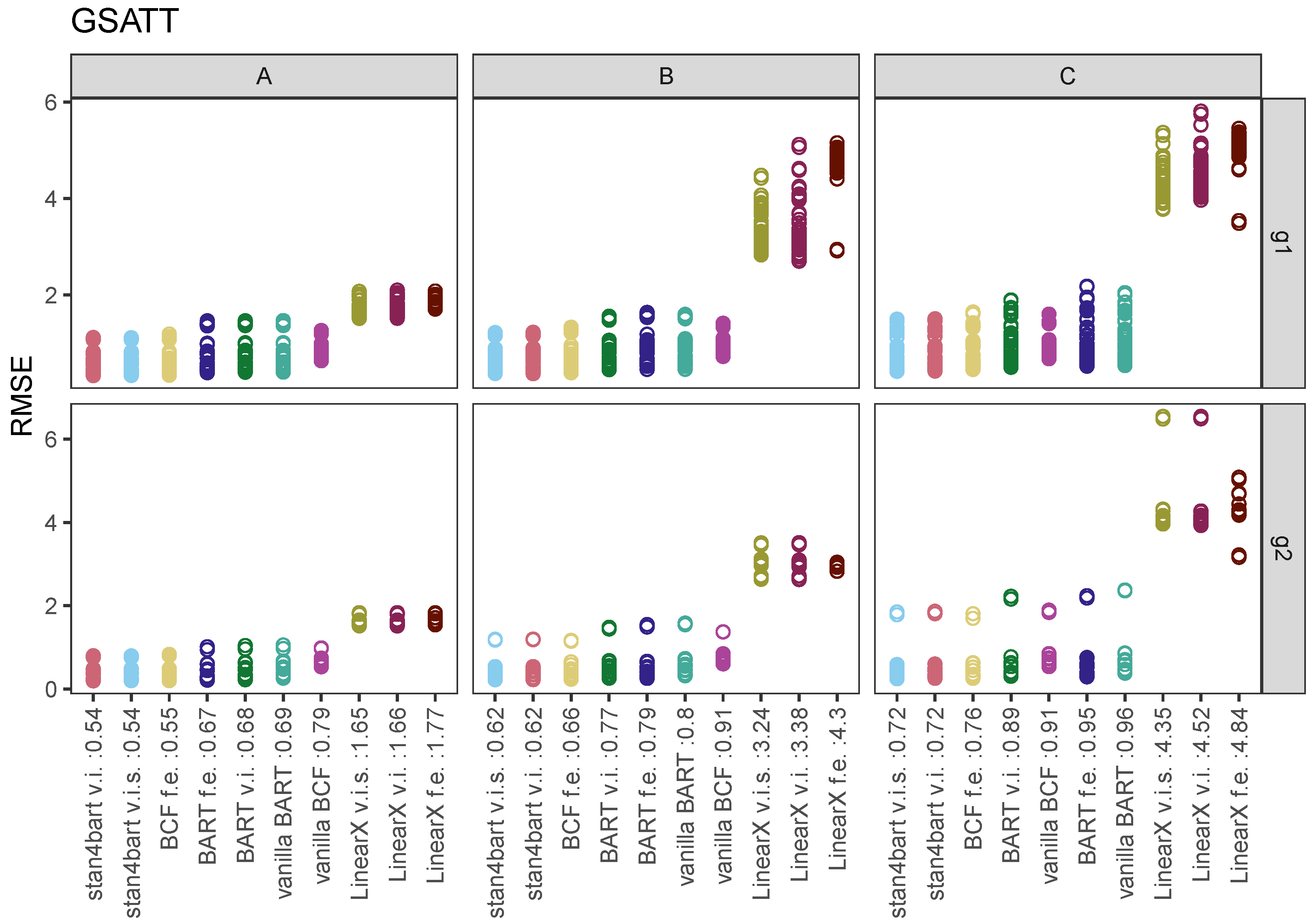
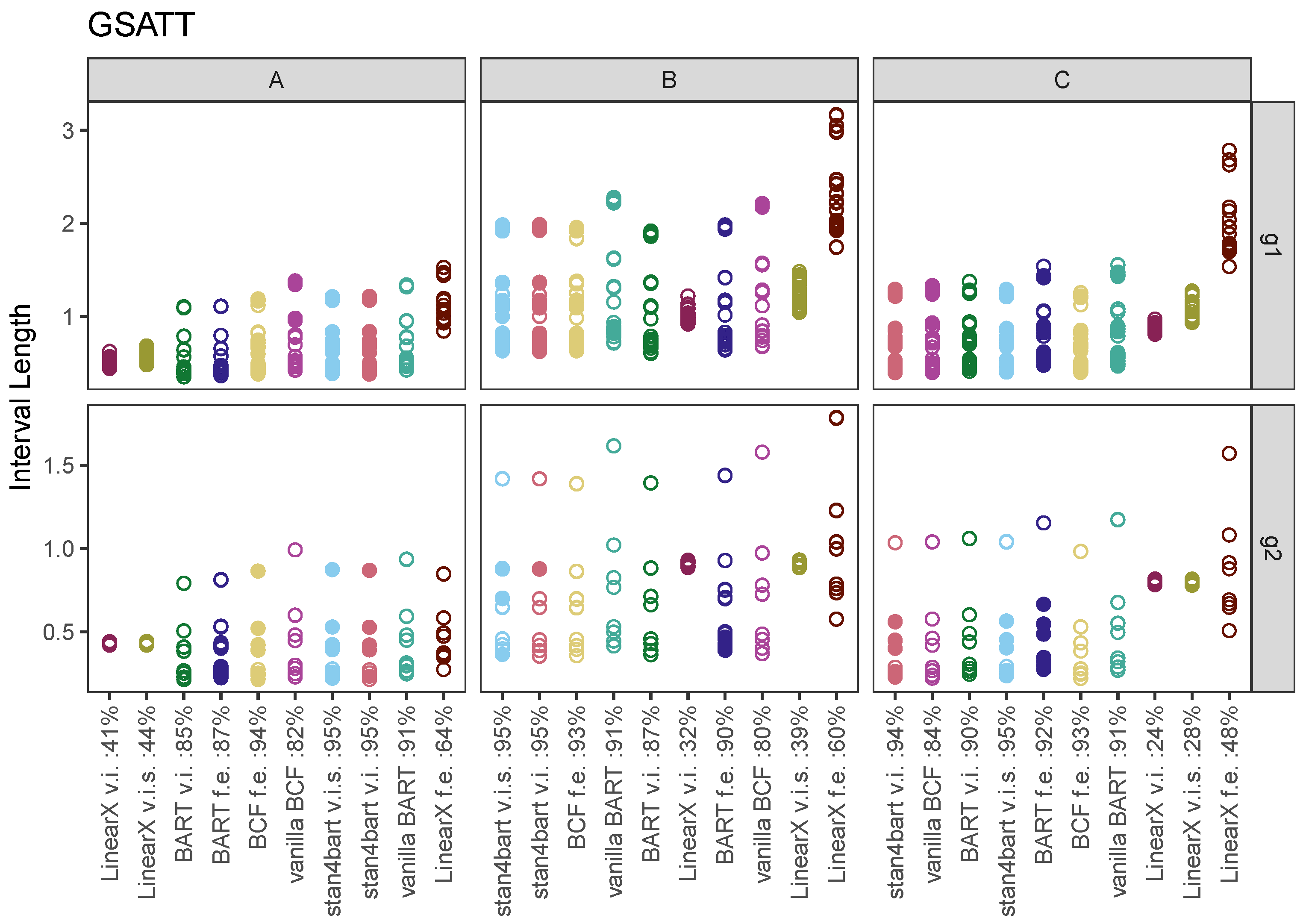
7.2. GSATT
7.3. iCATEs
8. Discussion
Author Contributions
Funding
Institutional Review Board Statement
Data Availability Statement
Conflicts of Interest
References
- Hill, J. Bayesian nonparametric modeling for causal inference. J. Comput. Graph. Stat. 2011, 20, 217–240. [Google Scholar] [CrossRef]
- LeDell, E. h2oEnsemble: H2O Ensemble Learning, R Package Version 0.1.8. 2016.
- Wager, S.; Athey, S. Estimation and Inference of Heterogeneous Treatment Effects using Random Forests. J. Am. Stat. Assoc. 2018, 113, 1228–1242. [Google Scholar] [CrossRef]
- Künzel, S.R.; Sekhon, J.S.; Bickel, P.J.; Yu, B. Metalearners for estimating heterogeneous treatment effects using machine learning. Proc. Natl. Acad. Sci. USA 2019, 116, 4156–4165. [Google Scholar] [CrossRef] [PubMed]
- Ju, C.; Gruber, S.; Lendle, S.D.; Chambaz, A.; Franklin, J.M.; Wyss, R.; Schneeweiss, S.; van der Laan, M.J. Scalable collaborative targeted learning for high-dimensional data. Stat. Methods Med. Res. 2019, 28, 532–554. [Google Scholar] [CrossRef] [PubMed]
- Zeldow, B.; Lo Re, V.R.; Roy, J. A Semiparametric Modeling Approach Using Bayesian Additive Regression Trees with an Application to Evaluate Heterogeneous Treatment Effects. Ann. Appl. Stat. 2019, 13, 1989–2010. [Google Scholar] [CrossRef]
- Hahn, P.R.; Murray, J.S.; Carvalho, C.M. Bayesian Regression Tree Models for Causal Inference: Regularization, Confounding, and Heterogeneous Effects (with Discussion). Bayesian Anal. 2020, 15, 965–2020. [Google Scholar] [CrossRef]
- Dehejia, R.H. Was There a Riverside Miracle? A Hierarchical Framework for Evaluating Programs with Grouped Data. J. Bus. Econ. Stat. 2003, 21, 1–11. [Google Scholar] [CrossRef][Green Version]
- Gelman, A.; Hill, J. Data Analysis Using Regression and Multilevel/Hierarchical Models; Cambridge University Press: New York, NY, USA, 2007. [Google Scholar]
- Hill, J. The SAGE Handbook of Multilevel Modeling; Chapter Multilevel Models and Causal Inference; SAGE: London, UK, 2013; pp. 1248–1318. [Google Scholar]
- Lin, W. Agnostic notes on regression adjustments to experimental data: Reexamining Freedman’s critique. Ann. Appl. Stat. 2013, 7, 295–318. [Google Scholar] [CrossRef]
- Chipman, H.; George, E.; McCulloch, R. Bayesian Ensemble Learning. In Advances in Neural Information Processing Systems 19; Schölkopf, B., Platt, J., Hoffman, T., Eds.; MIT Press: Cambridge, MA, USA, 2007. [Google Scholar]
- Chipman, H.A.; George, E.I.; McCulloch, R.E. BART: Bayesian Additive Regression Trees. Ann. Appl. Stat. 2010, 4, 266–298. [Google Scholar] [CrossRef]
- Dorie, V. dbarts: Discrete Bayesian Additive Regression Trees Sampler, R Package Version 0.9-22. 2022.
- Dorie, V.; Hill, J.; Shalit, U.; Scott, M.; Cervone, D. Automated versus do-it-yourself methods for causal inference: Lessons learned from a data analysis competition. Stat. Sci. 2019, 34, 43–68. [Google Scholar] [CrossRef]
- Bonato, V.; Baladandayuthapani, V.; Broom, B.M.; Sulman, E.P.; Aldape, K.D.; Do, K.A. Bayesian ensemble methods for survival prediction in gene expression data. Bioinformatics 2010, 27, 359–367. [Google Scholar] [CrossRef] [PubMed]
- Pratola, M.; Chipman, H.; George, E.; McCulloch, R. Heteroscedastic BART using multiplicative regression trees. J. Comput. Graph. Stat. 2020, 29, 405–417. [Google Scholar] [CrossRef]
- Linero, A.R.; Sinha, D.; Lipsitz, S.R. Semiparametric mixed-scale models using shared Bayesian forests. Biometrics 2020, 76, 131–144. [Google Scholar] [CrossRef]
- George, E.; Laud, P.; Logan, B.; McCulloch, R.; Sparapani, R. Fully nonparametric Bayesian additive regression trees. In Topics in Identification, Limited Dependent Variables, Partial Observability, Experimentation, and Flexible Modeling: Part B; Emerald Publishing Limited: Bingley, UK, 2019; Volume 40, pp. 89–110. [Google Scholar]
- Murray, J.S. Log-Linear Bayesian Additive Regression Trees for Multinomial Logistic and Count Regression Models. J. Am. Stat. Assoc. 2021, 116, 756–769. [Google Scholar] [CrossRef]
- Hill, J.L.; Weiss, C.; Zhai, F. Challenges with Propensity Score Strategies in a High-Dimensional Setting and a Potential Alternative. Multivar. Behav. Res. 2011, 46, 477–513. [Google Scholar] [CrossRef] [PubMed]
- Hill, J.; Su, Y.S. Assessing lack of common support in causal inference using Bayesian nonparametrics: Implications for evaluating the effect of breastfeeding on children’s cognitive outcomes. Ann. Appl. Stat. 2013, 7, 1386–1420. [Google Scholar] [CrossRef]
- Dorie, V.; Carnegie, N.B.; Harada, M.; Hill, J. A flexible, interpretable framework for assessing sensitivity to unmeasured confounding. Stat. Med. 2016, 35, 3453–3470. [Google Scholar] [CrossRef]
- Kern, H.L.; Stuart, E.A.; Hill, J.L.; Green, D.P. Assessing methods for generalizing experimental impact estimates to target samples. J. Res. Educ. Eff. 2016, 9, 103–127. [Google Scholar]
- Wendling, T.; Jung, K.; Callahan, A.; Schuler, A.; Shah, N.; Gallego, B. Comparing methods for estimation of heterogeneous treatment effects using observational data from health care databases. Stat. Med. 2018, 37, 3309–3324. [Google Scholar] [CrossRef]
- Sparapani, R.; Spanbauer, C.; McCulloch, R. Nonparametric Machine Learning and Efficient Computation with Bayesian Additive Regression Trees: The BART R Package. J. Stat. Softw. 2021, 97, 1–66. [Google Scholar] [CrossRef]
- Bisbee, J. BARP: Improving Mister P Using Bayesian Additive Regression Trees. Am. Political Sci. Rev. 2019, 113, 1060–1065. [Google Scholar] [CrossRef]
- Yeager, D.S.; Hanselman, P.; Walton, G.M.; Murray, J.S.; Crosnoe, R.; Muller, C.; Tipton, E.; Schneider, B.; Hulleman, C.S.; Hinojosa, C.P.; et al. A national experiment reveals where a growth mindset improves achievement. Nature 2019, 573, 364–369. [Google Scholar] [CrossRef]
- Yeager, D.; Bryan, C.; Gross, J.; Murray, J.S.; Cobb, D.K.; Santos, P.H.F.; Gravelding, H.; Johnson, M.; Jamieson, J.P. A synergistic mindsets intervention protects adolescents from stress. Nature 2022, 607, 512–520. [Google Scholar] [CrossRef] [PubMed]
- Yeager, D.S.; Carroll, J.M.; Buontempo, J.; Cimpian, A.; Woody, S.; Crosnoe, R.; Muller, C.; Murray, J.; Mhatre, P.; Kersting, N.; et al. Teacher Mindsets Help Explain Where a Growth-Mindset Intervention Does and Doesn’t Work. Psychol. Sci. 2022, 33, 18–32. [Google Scholar] [CrossRef] [PubMed]
- Suk, Y.; Kang, H. Robust Machine Learning for Treatment Effects in Multilevel Observational Studies Under Cluster-level Unmeasured Confounding. Psychometrika 2022, 87, 310–343. [Google Scholar] [CrossRef] [PubMed]
- Spanbauer, C.; Sparapani, R. Nonparametric machine learning for precision medicine with longitudinal clinical trials and Bayesian additive regression trees with mixed models. Stat. Med. 2021, 40, 2665–2691. [Google Scholar] [CrossRef] [PubMed]
- Tan, Y.V.; Flannagan, C.A.C.; Elliott, M.R. Predicting human-driving behavior to help driverless vehicles drive: Random intercept Bayesian additive regression trees. Stat. Its Interface 2018, 11, 557–572. [Google Scholar] [CrossRef]
- Rubin, D.B. Using Multivariate Matched Sampling and Regression Adjustment to Control Bias in Observational Studies. J. Am. Stat. Assoc. 1979, 74, 318–328. [Google Scholar]
- Holland, P. Statistics and Causal Inference. J. Am. Stat. Assoc. 1986, 81, 945–970. [Google Scholar] [CrossRef]
- Vegetabile, B.G. On the Distinction Between “Conditional Average Treatment Effects” (CATE) and “Individual Treatment Effects” (ITE) Under Ignorability Assumptions. arXiv 2021, arXiv:2108.04939. [Google Scholar]
- Carnegie, N.; Dorie, V.; Hill, J. Examining treatment effect heterogeneity using BART. Obs. Stud. 2019, 76, 491–511. [Google Scholar] [CrossRef]
- Carnegie, N.B.; Harada, M.; Hill, J. Assessing sensitivity to unmeasured confounding using a simulated potential confounder. J. Res. Educ. Eff. 2016, 9, 395–420. [Google Scholar] [CrossRef]
- Rubin, D.B. Bayesian Inference for Causal Effects: The role of randomization. Ann. Stat. 1978, 6, 34–58. [Google Scholar] [CrossRef]
- Team, S.D. Stan Modeling Language Users Guide and Reference Manual; Version 2.29. 2022. Available online: https://mc-stan.org/docs/2_29/stan-users-guide/ (accessed on 14 August 2022).
- Hoffman, M.D.; Gelman, A. The No-U-Turn Sampler: Adaptively Setting Path Lengths in Hamiltonian Monte Carlo. J. Mach. Learn. Res. 2014, 15, 1593–1623. [Google Scholar]
- Betancourt, M. A conceptual introduction to Hamiltonian Monte Carlo. arXiv 2017, arXiv:1701.02434. [Google Scholar]
- Neal, R.M. MCMC using Hamiltonian dynamics. Handb. Markov Chain. Monte Carlo 2011, 2, 2. [Google Scholar]
- Bates, D.; Mächler, M.; Bolker, B.; Walker, S. Fitting Linear Mixed-Effects Models Using lme4. J. Stat. Softw. 2015, 67, 1–48. [Google Scholar] [CrossRef]
- Lewandowski, D.; Kurowicka, D.; Joe, H. Generating random correlation matrices based on vines and extended onion method. J. Multivar. Anal. 2009, 100, 1989–2001. [Google Scholar] [CrossRef]
- Bates, D.; Kliegl, R.; Vasishth, S.; Baayen, H. Parsimonious Mixed Models. arXiv 2015, arXiv:1506.04967. [Google Scholar]
- Bleich, J.; Kapelner, A.; George, E.I.; Jensen, S.T. Variable selection for BART: An application to gene regulation. Ann. Appl. Stat. 2014, 8, 1750–1781. [Google Scholar] [CrossRef]
- Casella, G.; George, E.I. Explaining the Gibbs Sampler. Am. Stat. 1992, 46, 167–174. [Google Scholar]
- Stan Development Team. RStan: The R Interface to Stan, R Package Version 2.21.5. 2022.
- Tan, Y.V.; Roy, J. Bayesian additive regression trees and the General BART model. Stat. Med. 2019, 38, 5048–5069. [Google Scholar] [CrossRef] [PubMed]
- Guidotti, R.; Monreale, A.; Ruggieri, S.; Turini, F.; Giannotti, F.; Pedreschi, D. A Survey of Methods for Explaining Black Box Models. ACM Comput. Surv. 2018, 51, 1–41. [Google Scholar] [CrossRef]
- Liu, J.S.; Wu, Y.N. Parameter Expansion for Data Augmentation. J. Am. Stat. Assoc. 1999, 94, 1264–1274. [Google Scholar] [CrossRef]
- Meng, X.L.; van Dyk, D. Seeking efficient data augmentation schemes via conditional and marginal augmentation. Biometrika 1999, 86, 301–320. [Google Scholar] [CrossRef]
- Gelman, A.; van Dyk, D.A.; Huang, Z.; Boscardin, J.W. Using Redundant Parameterizations to Fit Hierarchical Models. J. Comput. Graph. Stat. 2008, 17, 95–122. [Google Scholar] [CrossRef]
- Carnegie, N. Contributions of Model Features to BART Causal Inference Performance Using ACIC 2016 Competition Data. Stat. Sci. 2019, 34, 90–93. [Google Scholar] [CrossRef]
- Middleton, J.; Scott, M.; Diakow, R.; Hill, J. Bias Amplification and Bias Unmasking. Political Anal. 2016, 24, 307–323. [Google Scholar] [CrossRef]
- Scott, M.; Diakow, R.; Hill, J.; Middleton, J. Potential for Bias Inflation with Grouped Data: A Comparison of Estimators and a Sensitivity Analysis Strategy. Obs. Stud. 2018, 4, 111–149. [Google Scholar] [CrossRef]
- Infant Health and Development Program. Enhancing the outcomes of low-birth-weight, premature infants. J. Am. Med Assoc. 1990, 22, 3035–3042. [Google Scholar]
- Brooks-Gunn, J.; Liaw, F.R.; Klebanov, P.K. Effects of early intervention on cognitive function of low birth weight preterm infants. J. Pediatr. 1991, 120, 350–359. [Google Scholar] [CrossRef] [PubMed]


Publisher’s Note: MDPI stays neutral with regard to jurisdictional claims in published maps and institutional affiliations. |
© 2022 by the authors. Licensee MDPI, Basel, Switzerland. This article is an open access article distributed under the terms and conditions of the Creative Commons Attribution (CC BY) license (https://creativecommons.org/licenses/by/4.0/).
Share and Cite
Dorie, V.; Perrett, G.; Hill, J.L.; Goodrich, B. Stan and BART for Causal Inference: Estimating Heterogeneous Treatment Effects Using the Power of Stan and the Flexibility of Machine Learning. Entropy 2022, 24, 1782. https://doi.org/10.3390/e24121782
Dorie V, Perrett G, Hill JL, Goodrich B. Stan and BART for Causal Inference: Estimating Heterogeneous Treatment Effects Using the Power of Stan and the Flexibility of Machine Learning. Entropy. 2022; 24(12):1782. https://doi.org/10.3390/e24121782
Chicago/Turabian StyleDorie, Vincent, George Perrett, Jennifer L. Hill, and Benjamin Goodrich. 2022. "Stan and BART for Causal Inference: Estimating Heterogeneous Treatment Effects Using the Power of Stan and the Flexibility of Machine Learning" Entropy 24, no. 12: 1782. https://doi.org/10.3390/e24121782
APA StyleDorie, V., Perrett, G., Hill, J. L., & Goodrich, B. (2022). Stan and BART for Causal Inference: Estimating Heterogeneous Treatment Effects Using the Power of Stan and the Flexibility of Machine Learning. Entropy, 24(12), 1782. https://doi.org/10.3390/e24121782