


Optimal Security Protection Strategy Selection Model Based on Q-Learning Particle Swarm Optimization


Abstract
1. Introduction
2. Related Work
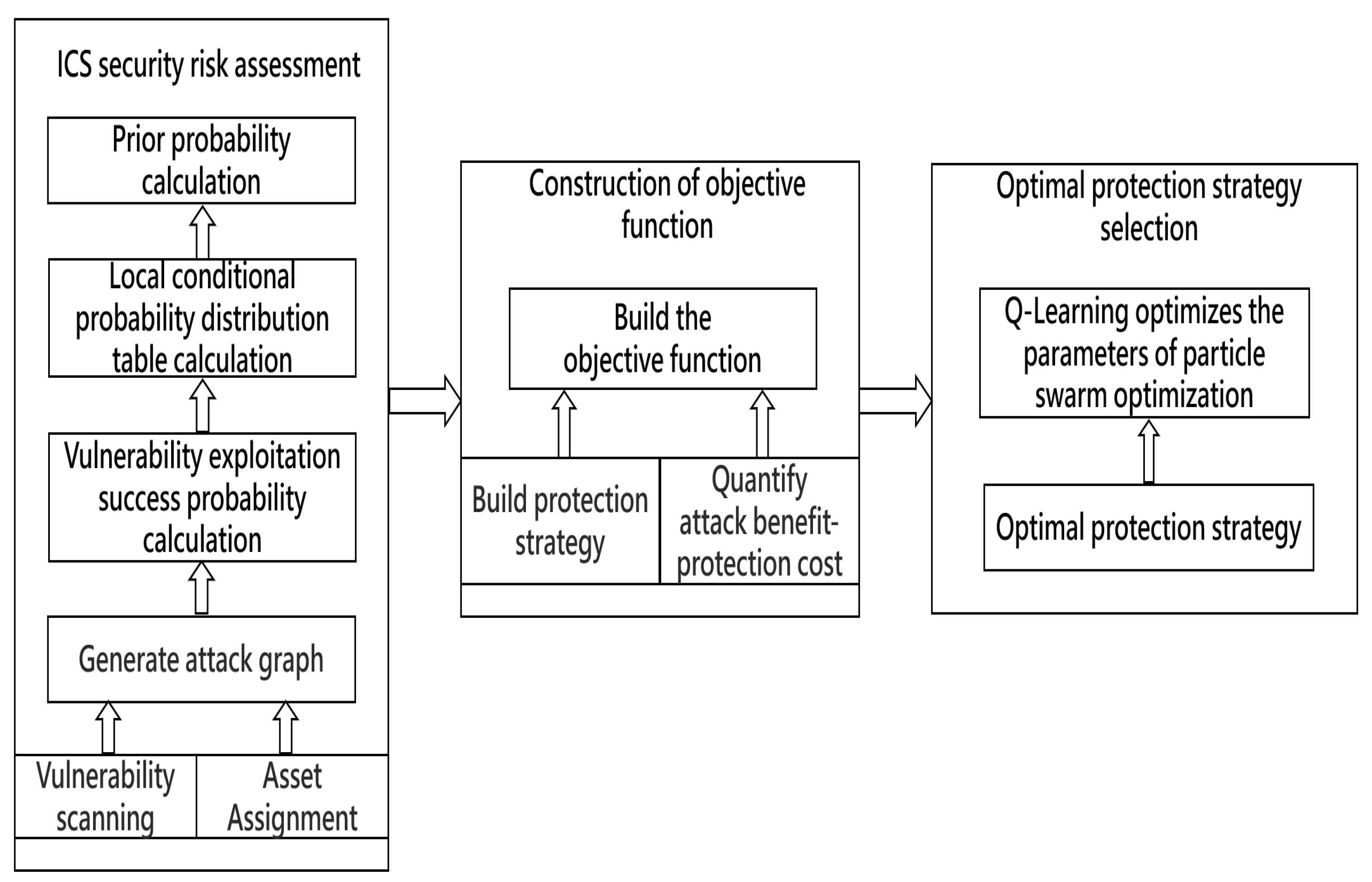
3. Model Framework
- (1)
- ICS security risk assessment: First, we build a Bayesian attack graph based on the network configuration and asset information of the ICS [36], then calculate the exploit success rate of each edge of the attack graph, and construct the local conditional probability distribution (LCPD) table according to the exploit success rate. Finally, the prior probabilities of all attribute nodes being attacked are calculated [37];
- (2)
- Construction of the objective function: Firstly, we construct all possible protection strategies based on the network configuration and asset information of the ICS, then quantify the attack benefit and protection cost, and finally construct the objective function based on both the attack benefit and protection cost;
- (3)
- Optimal protection strategy selection: First, we design the Q-Learning particle swarm optimization algorithm (QLPSO), then solve the objective function using the QLPSO, and finally find the optimal protection strategy.
4. ICS Security Risk Assessment
4.1. Definition of Bayesian Attack Graph
- (1)
- is the set of all attribute nodes of the attack graph.
- (2)
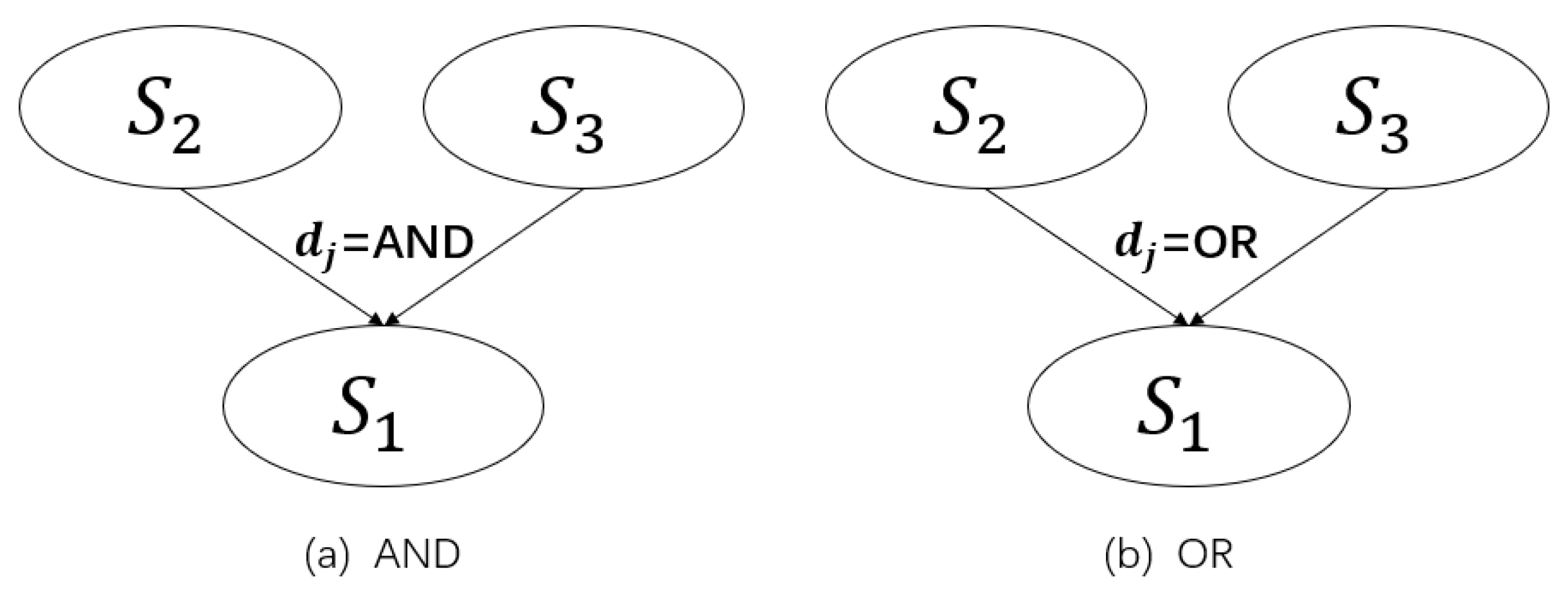
- is the set of all directed edges of the attack graph, where has two end nodes and , and is the parent node and the child node.
- (3)
- means atomic attack. means that the attack has been launched, otherwise .
- (4)
- is the set of the probabilities that the attribute nodes can be attacked. indicates the success probability of attribute node of being attacked.
4.2. Calculation of Success Probability of Vulnerability Exploitation
4.3. Calculation of Local Conditional Probability Distribution (LCPD)
4.4. Prior Probability Calculation
5. Construction of Objective Function
5.1. Protection Strategy
5.2. Attack Benefit
5.3. Attack Benefit-Protection Cost Objective Function
6. Q-Learning Particle Swarm Optimization Algorithm
6.1. Particle Swarm Optimization
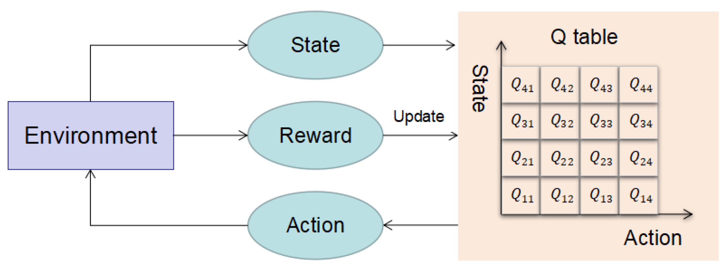
6.2. Q-Learning
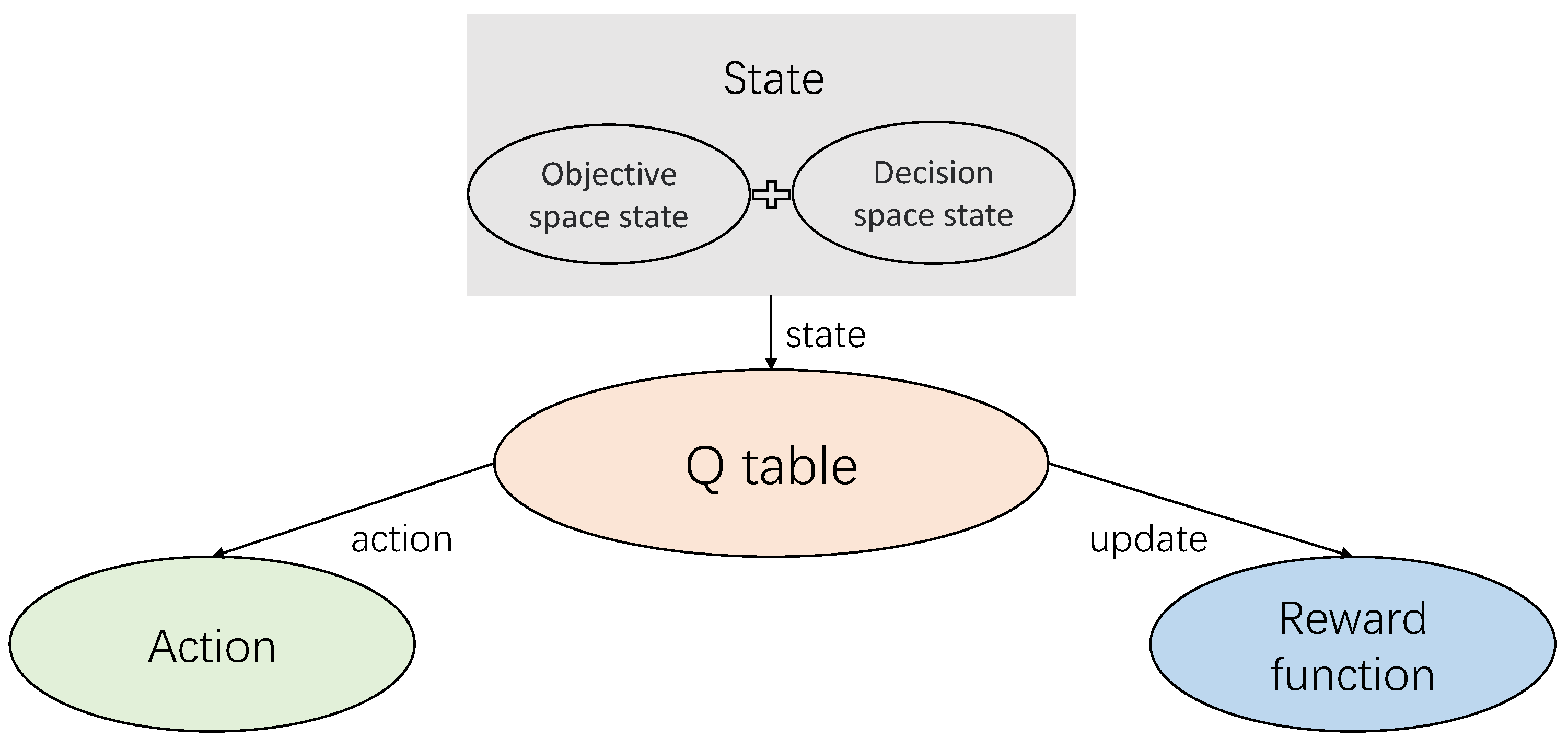
6.3. Q-Learning Particle Swarm Optimization (QLPSO)
- (1)
- States
- (2)
- Action
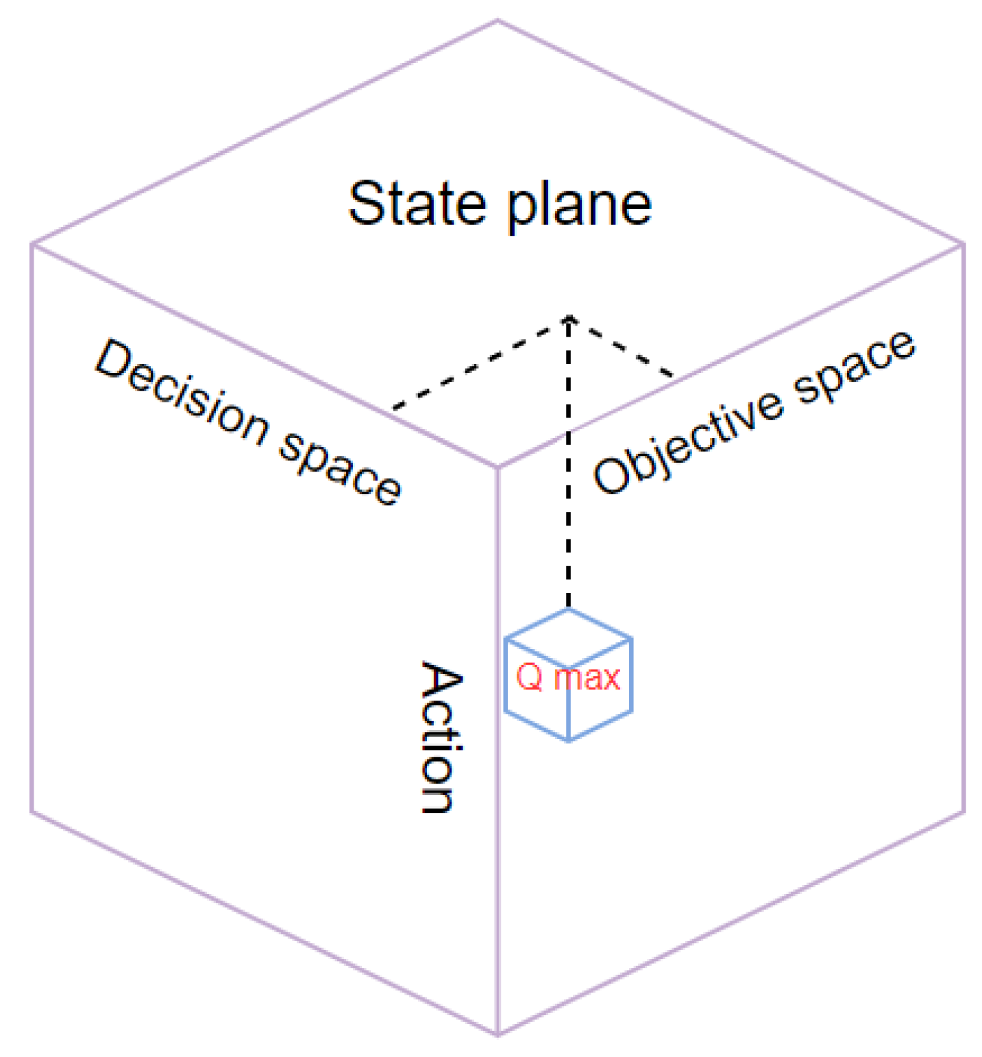
- (3)
- Q table
- (4)
- Rewards
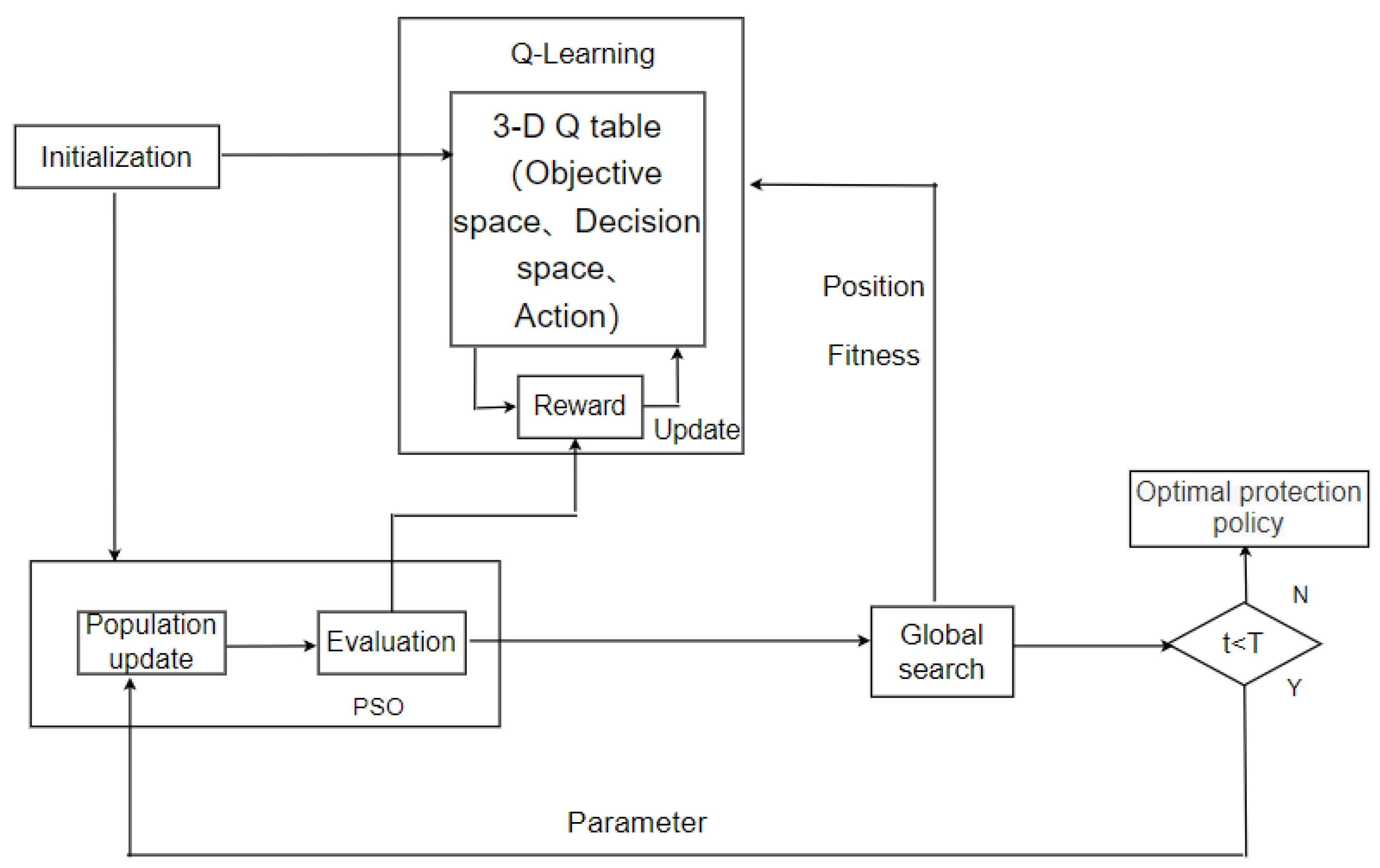
- (1)
- Initialize the population and Q table;
- (2)
- The state of each particle is determined according to its position in the objective space and decision space;
- (3)
- The action (parameter) of the particle is determined using the Q table;
- (4)
- Update the particles according to the parameters determined in the previous step;
- (5)
- Update the Q table according to the reward function;
- (6)
- These steps are repeated for all particles in each generation until the number of iterations is reached.

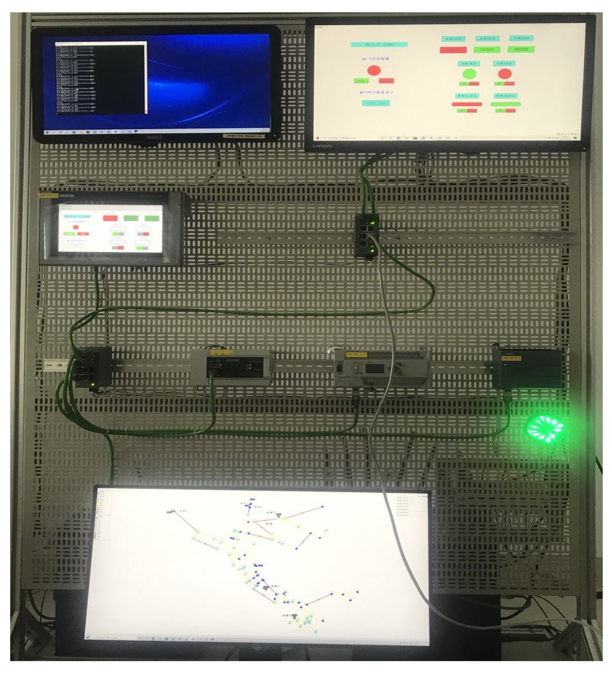
7. Experimental
7.1. Experimental Scenario
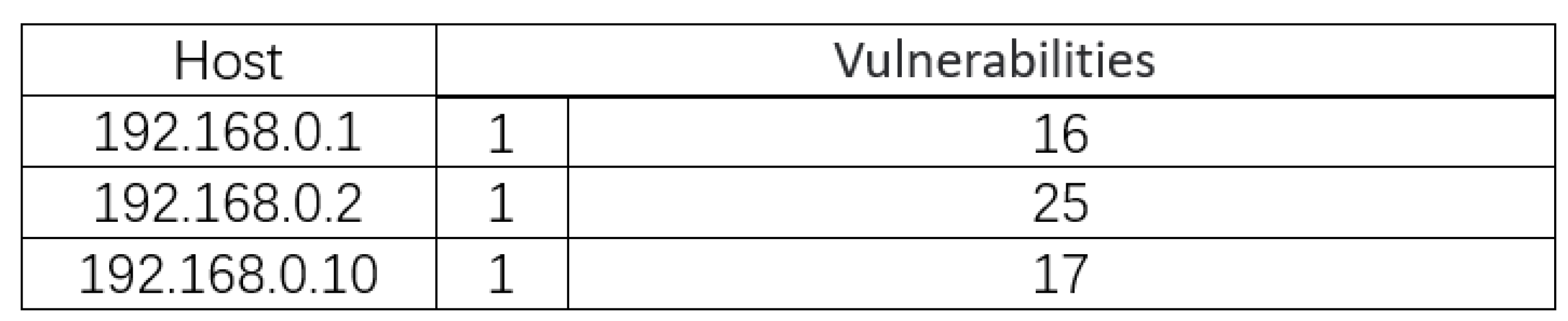
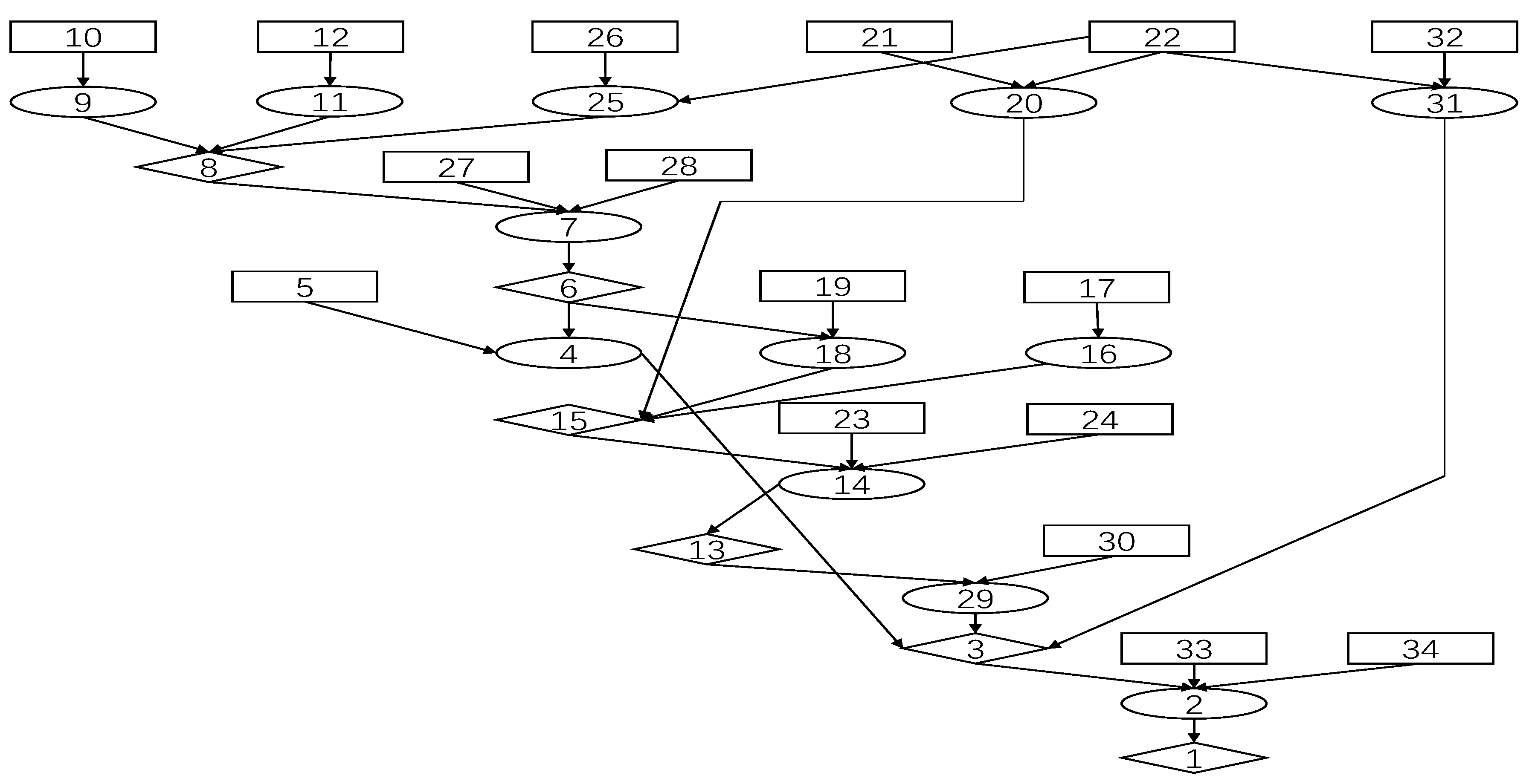
7.2. Generating a Bayesian Attack Graph
7.3. Attack Benefits and Protection Costs
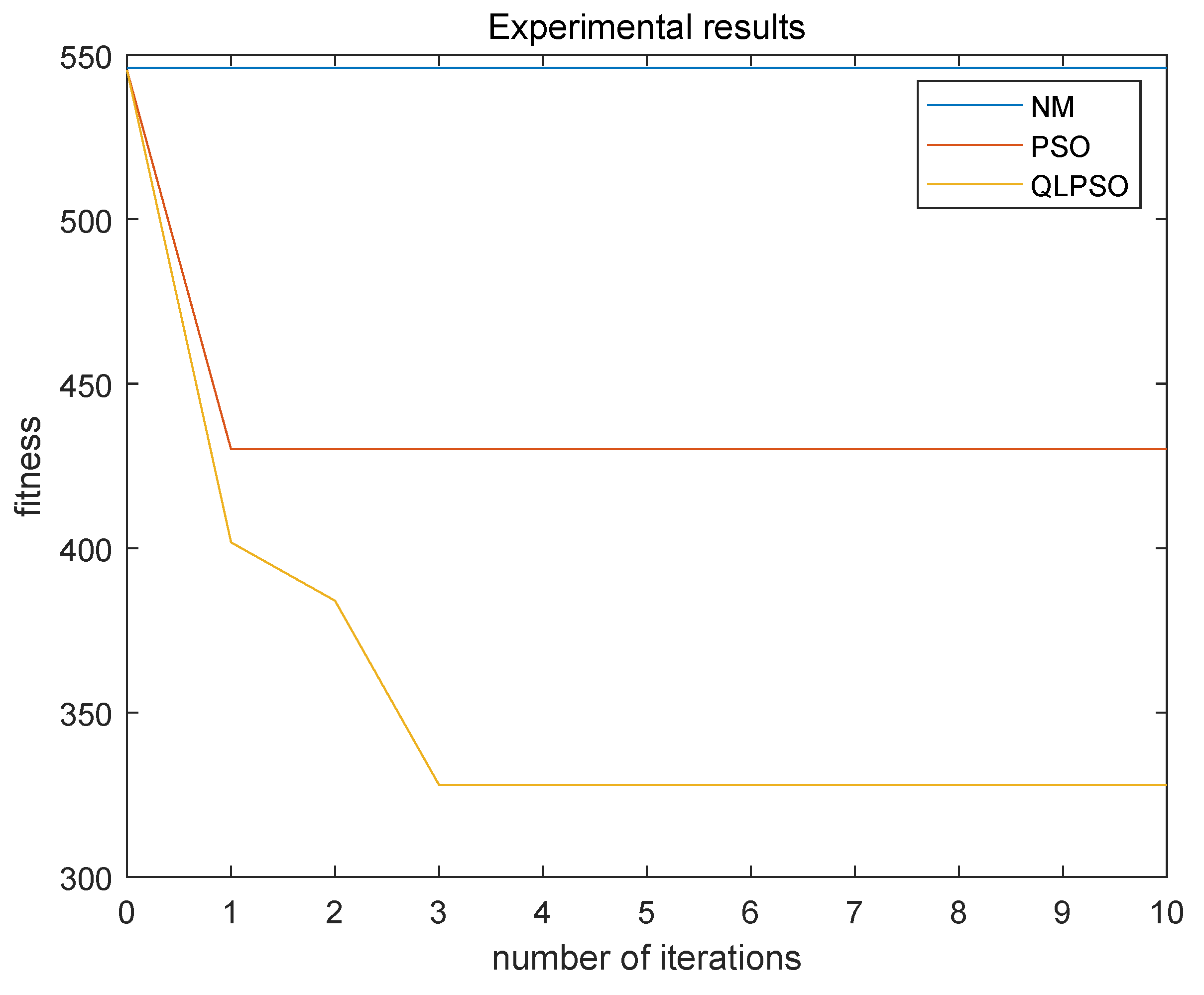
7.4. Experimental Results
8. Conclusions
Author Contributions
Funding
Institutional Review Board Statement
Data Availability Statement
Conflicts of Interest
References
- Brändle, M.; Naedele, M. Security for process control systems: An overview. IEEE Secur. Priv. 2008, 6, 24–29. [Google Scholar] [CrossRef]
- Fan, X.; Fan, K.; Wang, Y.; Zhou, R. Overview of cyber-security of industrial control system. In Proceedings of the 2015 international conference on cyber security of smart cities, industrial control system and communications (SSIC), Shanghai, China, 5–7 August 2015; pp. 1–7. [Google Scholar]
- Wilhoit, K. Who’s really attacking your ICS equipment? Trend Micro 2013, 10. [Google Scholar]
- Clarke, G.; Reynders, D.; Wright, E. Practical Modern SCADA Protocols: DNP3, 60870.5 and Related Systems; Elsevier: Newnes, Australia, 2004. [Google Scholar]
- van Schuppen, J.H.; Boutin, O.; Kempker, P.L.; Komenda, J.; Masopust, T.; Pambakian, N.; Ran, A.C. Control of distributed systems: Tutorial and overview. Eur. J. Control 2011, 17, 579–602. [Google Scholar] [CrossRef]
- Babu, B.; Ijyas, T.; Muneer, P.; Varghese, J. Security issues in SCADA based industrial control systems. In Proceedings of the 2017 2nd International Conference on Anti-Cyber Crimes (ICACC), Abha, Saudi Arabia, 26–27 March 2017; pp. 47–51. [Google Scholar]
- Wang, Y. SCM/ERP/MES/PCS integration for process enterprise. In Proceedings of the 29th Chinese Control Conference, Beijing, China, 29–31 July 2010; pp. 5329–5332. [Google Scholar]
- Li, Z.; Shahidehpour, M.; Aminifar, F. Cybersecurity in distributed power systems. Proc. IEEE 2017, 105, 1367–1388. [Google Scholar] [CrossRef]
- Cruz, T.; Rosa, L.; Proença, J.; Maglaras, L.; Aubigny, M.; Lev, L.; Jiang, J.; Simões, P. A cybersecurity detection framework for supervisory control and data acquisition systems. IEEE Trans. Ind. Inform. 2016, 12, 2236–2246. [Google Scholar] [CrossRef]
- Chen, T.M.; Abu-Nimeh, S. Lessons from stuxnet. Computer 2011, 44, 91–93. [Google Scholar] [CrossRef]
- Sun, C.C.; Hahn, A.; Liu, C.C. Cyber security of a power grid: State-of-the-art. Int. J. Electr. Power Energy Syst. 2018, 99, 45–56. [Google Scholar] [CrossRef]
- Zhao, D.; Wang, L.; Wang, Z.; Xiao, G. Virus propagation and patch distribution in multiplex networks: Modeling, analysis, and optimal allocation. IEEE Trans. Inf. Forensics Secur. 2019, 14, 1755–1767. [Google Scholar] [CrossRef]
- Stouffer, K.; Falco, J.; Scarfone, K. Guide to industrial control systems (ICS) security. NIST Spec. Publ. 2011, 800, 16. [Google Scholar]
- David, A. Multiple Efforts to Secure Control Systems Are under Way, But Challenges Remain; Technical report; US Government Accountability Office (US GAO): Washington DC, USA, 2007. [Google Scholar]
- Zhao, D.; Xiao, G.; Wang, Z.; Wang, L.; Xu, L. Minimum dominating set of multiplex networks: Definition, application, and identification. IEEE Trans. Syst. Man Cybern. Syst. 2021, 51, 7823–7837. [Google Scholar] [CrossRef]
- Shameli-Sendi, A.; Desfossez, J.; Dagenais, M.; Jabbarifar, M. A Retroactive-Burst Framework for Automated Intrusion Response System. J. Comput. Netw. Commun. 2013, 2013, 134760.1–134760.8. [Google Scholar] [CrossRef]
- Deb, K.; Pratap, A.; Agarwal, S.; Meyarivan, T. A fast and elitist multiobjective genetic algorithm: NSGA-II. IEEE Trans. Evol. Comput. 2002, 6, 182–197. [Google Scholar] [CrossRef]
- Gonzalez-Granadillo, G.; Garcia-Alfaro, J.; Alvarez, E.; El-Barbori, M.; Debar, H. Selecting optimal countermeasures for attacks against critical systems using the attack volume model and the RORI index. Comput. Electr. Eng. 2015, 47, 13–34. [Google Scholar] [CrossRef]
- Miehling, E.; Rasouli, M.; Teneketzis, D. Optimal defense policies for partially observable spreading processes on Bayesian attack graphs. In Proceedings of the Second ACM Workshop on Moving Target Defense, Denver, CO, USA, 12 October 2015; pp. 67–76. [Google Scholar]
- Jaquith, A. Security Metrics: Replacing Fear, Uncertainty, and Doubt; Pearson Education: London, UK, 2007. [Google Scholar]
- Bandyopadhyay, S.; Saha, S. Some single-and multiobjective optimization techniques. In Unsupervised Classification; Springer: Berlin/Heidelberg, Germany, 2013; pp. 17–58. [Google Scholar]
- Poolsappasit, N.; Dewri, R.; Ray, I. Dynamic security risk management using bayesian attack graphs. IEEE Trans. Dependable Secur. Comput. 2011, 9, 61–74. [Google Scholar] [CrossRef]
- Yigit, B.; Gür, G.; Alagöz, F. Cost-aware network hardening with limited budget using compact attack graphs. In Proceedings of the 2014 IEEE Military Communications Conference, Baltimore, MD, USA, 6–8 October 2014; pp. 152–157. [Google Scholar]
- Lei, C.; Ma, D.H.; Zhang, H.Q. Optimal strategy selection for moving target defense based on Markov game. IEEE Access 2017, 5, 156–169. [Google Scholar] [CrossRef]
- Herold, N.; Wachs, M.; Posselt, S.A.; Carle, G. An optimal metric-aware response selection strategy for intrusion response systems. In Proceedings of the International Symposium on Foundations and Practice of Security, Quebec City, QC, Canada, 24–25 October 2016; Springer: Berlin/Heidelberg, Germany, 2016; pp. 68–84. [Google Scholar]
- Butler, S.A. Security attribute evaluation method: A cost-benefit approach. In Proceedings of the 24th International Conference on Software Engineering, Orlando, FL, USA, 19–25 May 2002; pp. 232–240. [Google Scholar]
- Butler, S.A.; Fischbeck, P. Multi-attribute risk assessment. In Proceedings of the Symposium on Requirements Engineering for Information Security, Raleigh, NC, USA, 16 October 2002; Volume 2. [Google Scholar]
- Roy, A.; Kim, D.S.; Trivedi, K.S. Scalable optimal countermeasure selection using implicit enumeration on attack countermeasure trees. In Proceedings of the IEEE/IFIP International Conference on Dependable Systems and Networks (DSN 2012), Boston, MA, USA, 25–28 June 2012; pp. 1–12. [Google Scholar]
- Viduto, V.; Maple, C.; Huang, W.; López-Peréz, D. A novel risk assessment and optimisation model for a multi-objective network security countermeasure selection problem. Decis. Support Syst. 2012, 53, 599–610. [Google Scholar] [CrossRef]
- Dewri, R.; Ray, I.; Poolsappasit, N.; Whitley, D. Optimal security hardening on attack tree models of networks: A cost-benefit analysis. Int. J. Inf. Secur. 2012, 11, 167–188. [Google Scholar] [CrossRef]
- Wang, S.; Zhang, Z.; Kadobayashi, Y. Exploring attack graph for cost-benefit security hardening: A probabilistic approach. Comput. Secur. 2013, 32, 158–169. [Google Scholar] [CrossRef]
- Kordy, B.; Wideł, W. How well can I secure my system? In Proceedings of the International Conference on Integrated Formal Methods, Turin, Italy, 20–22 September 2017; Springer: Berlin/Heidelberg, Germany, 2017; pp. 332–347. [Google Scholar]
- Fila, B.; Wideł, W. Exploiting attack–defense trees to find an optimal set of countermeasures. In Proceedings of the 2020 IEEE 33rd Computer Security Foundations Symposium (CSF), Boston, MA, USA, 22–26 June 2020; pp. 395–410. [Google Scholar]
- Speicher, P.; Steinmetz, M.; Künnemann, R.; Simeonovski, M.; Pellegrino, G.; Hoffmann, J.; Backes, M. Formally reasoning about the cost and efficacy of securing the email infrastructure. In Proceedings of the 2018 IEEE European Symposium on Security and Privacy (EuroS&P), London, UK, 24–26 April 2018; pp. 77–91. [Google Scholar]
- Zenitani, K. A multi-objective cost–benefit optimization algorithm for network hardening. Int. J. Inf. Secur. 2022, 21, 813–832. [Google Scholar] [CrossRef]
- Frigault, M.; Wang, L. Measuring network security using bayesian network-based attack graphs. In Proceedings of the 2008 32nd Annual IEEE International Computer Software and Applications Conference, Turku, Finland, 28 July–1 August 2008; pp. 698–703. [Google Scholar]
- Liu, Y.; Man, H. Network vulnerability assessment using Bayesian networks. In Proceedings of the Data Mining, Intrusion Detection, Information Assurance, and Data Networks Security 2005, Orlando, FL, USA, 28–29 March 2005; Volume 5812, pp. 61–71. [Google Scholar]
- Ou, X.; Govindavajhala, S.; Appel, A.W. MulVAL: A Logic-based Network Security Analyzer. In Proceedings of the USENIX Security Symposium, Baltimore, MD, USA, 31 July–5 August 2005; Volume 8, pp. 113–128. [Google Scholar]
- Mell, P.; Scarfone, K.; Romanosky, S. Common vulnerability scoring system. IEEE Secur. Priv. 2006, 4, 85–89. [Google Scholar] [CrossRef]
- Gao, N.; Gao, L.; He, Y.; Lei, Y.; Gao, Q. Dynamic security risk assessment model based on Bayesian attack graph. J. Sichuan Univ. (Eng. Sci. Ed.) 2016, 48, 111–118. [Google Scholar]
- Gao, N.; Gao, L.; Yiyue, H.E.; Wang, F. Optimal security hardening measures selection model based on Bayesian attack graph. Comput. Eng. Appl. 2016, 52, 125–130. [Google Scholar]
- Kennedy, J.; Eberhart, R. Particle swarm optimization. In Proceedings of the ICNN’95-International Conference on Neural Networks, Perth, WA, Australia, 27 November–1 December 1995; Volume 4, pp. 1942–1948. [Google Scholar]
- Clerc, M. Particle Swarm Optimization; John Wiley & Sons: Hoboken, NJ, USA, 2010; Volume 93. [Google Scholar]
- Jang, B.; Kim, M.; Harerimana, G.; Kim, J.W. Q-learning algorithms: A comprehensive classification and applications. IEEE Access 2019, 7, 133653–133667. [Google Scholar] [CrossRef]
- Watkins, C.J.; Dayan, P. Q-learning. Mach. Learn. 1992, 8, 279–292. [Google Scholar] [CrossRef]
- Clifton, J.; Laber, E. Q-learning: Theory and applications. Annu. Rev. Stat. Its Appl. 2020, 7, 279–301. [Google Scholar] [CrossRef]
- Liu, Y.; Lu, H.; Cheng, S.; Shi, Y. An adaptive online parameter control algorithm for particle swarm optimization based on reinforcement learning. In Proceedings of the 2019 IEEE Congress on Evolutionary Computation (CEC), Wellington, New Zealand, 10–13 June 2019; pp. 815–822. [Google Scholar]
- Abed-Alguni, B.H.; Paul, D.J.; Chalup, S.K.; Henskens, F.A. A comparison study of cooperative Q-learning algorithms for independent learners. Int. J. Artif. Intell. 2016, 14, 71–93. [Google Scholar]
- Meerza, S.I.A.; Islam, M.; Uzzal, M.M. Q-learning based particle swarm optimization algorithm for optimal path planning of swarm of mobile robots. In Proceedings of the 2019 1st International Conference on Advances in Science, Engineering and Robotics Technology (ICASERT), Dhaka, Bangladesh, 3–5 May 2019; pp. 1–5. [Google Scholar]
- Xu, L.; Wang, B.; Wu, X.; Zhao, D.; Zhang, L.; Wang, Z. Detecting Semantic Attack in SCADA System: A Behavioral Model Based on Secondary Labeling of States-Duration Evolution Graph. IEEE Trans. Netw. Sci. Eng. 2021, 9, 703–715. [Google Scholar] [CrossRef]


| Index | Rank | Score |
|---|---|---|
| local access | 0.395 | |
| Access Vector (AV) | adjacent network access | 0.646 |
| network accessible | 1.0 | |
| high | 0.35 | |
| Access complexity (AC) | medium | 0.61 |
| low | 0.71 | |
| multiple instances of authentication | 0.45 | |
| Authentication (AU) | single instance of authentication | 0.56 |
| no authentication | 0.704 |
| Relative Distance (Rd) | Decision Space State |
|---|---|
| 0 | DNearest |
| 0.25 | DNearer |
| 0.5 | DFarther |
| 0.75 | DFarthest |
| Single-Objective Problem Relative Fitness (Rf ) | Objective Space State |
|---|---|
| 0 | FSmallest |
| 0.25 | FSmaller |
| 0.5 | FLarger |
| 0.75 | FLargest |
| Search Status | Weight | Lp | Lb |
|---|---|---|---|
| Large scale search | 1 | 0.5 | 0.5 |
| Small scale search | 0.8 | 2 | 1 |
| Slow search | 0.6 | 1 | 2 |
| Fast search | 0.4 | 0.5 | 0.5 |
| Attribute Nodes | Prior Probability | Attribute Nodes | Prior Probability | Attribute Nodes | Priori Probability |
|---|---|---|---|---|---|
| 0.5000 | 0.1812 | 0.5000 | |||
| 0.5000 | 1.0000 | 1.0000 | |||
| 0.3967 | 0.5000 | 1.0000 | |||
| 1.0000 | 1.0000 | 1.0000 | |||
| 0.8372 | 0.3257 | 0.5000 | |||
| 1.0000 | 1.0000 | 0.5000 | |||
| 1.0000 | 0.6793 | 1.0000 | |||
| 1.0000 | 1.0000 | 0.9863 | |||
| 0.8000 | 1.0000 | 1.0000 | |||
| 0.9960 | 0.5814 | 1.0000 | |||
| 0.5641 | 1.0000 | 1.0000 | |||
| 0.9530 |
| Node | Node Information |
|---|---|
| 1 | execCode(192.168.0.1,someUser):0.3623 |
| 2 | RULE 2 (remote exploit of a server program):0.3623 |
| 3 | netAccess(192.168.0.1,udp,161):0.906 |
| 4 | RULE 5 (multi-hop access):0.3173 |
| 5 | hacl(192.168.0.10,192.168.0.1,udp,161):1.0 |
| 6 | execCode(192.168.0.10,someUser):0.3967 |
| 7 | RULE 2 (remote exploit of a server program):0.3967 |
| 8 | netAccess(192.168.0.10,udp,161):0.992 |
| 9 | RULE 5 (multi-hop access):0.8 |
| 10 | hacl(192.168.0.1,192.168.0.10,udp,161):1.0 |
| 11 | RULE 5 (multi-hop access):0.8 |
| 12 | hacl(192.168.0.2,192.168.0.10,udp,161):1.0 |
| 13 | execCode(192.168.0.2,someUser):0.389 |
| 14 | RULE 2 (remote exploit of a server program):0.389 |
| 15 | netAccess(192.168.0.2,udp,161):0.9727 |
| 16 | RULE 5 (multi-hop access):0.8 |
| 17 | hacl(192.168.0.1,192.168.0.2,udp,161):1.0 |
| 18 | RULE 5 (multi-hop access):0.3173 |
| 19 | hacl(192.168.0.10,192.168.0.2,udp,161):1.0 |
| 20 | RULE 6 (direct network access):0.8 |
| 21 | hacl(internet,192.168.0.2,udp,161):1.0 |
| 22 | attackerLocated(internet):1.0 |
| 23 | networkServiceInfo(192.168.0.2,sun sunos,udp,161,someUser):1.0 |
| 24 | vulExists(192.168.0.2,CVE-1999-0517,sun sunos,remoteExploit,privEscalation):0.4998 |
| 25 | RULE 6 (direct network access):0.8 |
| 26 | hacl(internet,192.168.0.10,udp,161):1.0 |
| 27 | networkServiceInfo(192.168.0.10, sun sunos,udp,161,someUser):1.0 |
| 28 | vulExists(192.168.0.10,CVE-1999-0517,sun sunos,remoteExploit,privEscalation):0.4998 |
| 29 | RULE 5 (multi-hop access):0.3112 |
| 30 | hacl(192.168.0.2,192.168.0.1,udp,161):1.0 |
| 31 | RULE 6 (direct network access):0.8 |
| 32 | hacl(internet,192.168.0.1,udp,161):1.0 |
| 33 | networkServiceInfo(192.168.0.1,sun sunos,udp,161,someUser):1.0 |
| 34 | vulExists(192.168.0.1,CVE-1999-0517,sun sunos,remoteExploit,privEscalation):0.4998 |
| Index | Weight () |
|---|---|
| Disable cost | 0.357 |
| Disconnect cost | 0.286 |
| Patch cost | 0.214 |
| Install cost | 0.143 |
| Protective Strategies | Protective Action | COST | Pi |
|---|---|---|---|
| Disconnect 192.168.0.1–192.168.0.10 | 14 | 0.25 | |
| Disconnect Disconnect 192.168.0.2–192.168.0.10 | 14 | 0.25 | |
| Disconnect Internet 192.168.0.10 | 15 | 0.30 | |
| Disconnect Internet 192.168.0.2 | 15 | 0.30 | |
| Disconnect Internet | 22 | 0.05 | |
| Disable Internet | 22 | 0.05 | |
| Disable Internet direct network access | 22 | 0.05 | |
| Disconnect Internet 192.168.0.1 | 15 | 0.30 | |
| Disable multi-hop access 192.168.0.10 | 12 | 0.10 | |
| Disable udp | 12 | 0.10 | |
| Disable direct network access 192.168.0.10 | 12 | 0.10 | |
| Disable direct network access 192.168.0.2 | 12 | 0.10 | |
| Disable direct network access 192.168.0.1 | 12 | 0.10 | |
| Disable netAccess 192.168.0.10 | 12 | 0.10 | |
| Disable networkService 192.168.0.10 | 18 | 0.45 | |
| Patch CVE-1999-0517 192.168.0.10 | 18 | 0.45 | |
| Disable service programs | 25 | 0.20 | |
| Disconnect 192.168.0.10–192.168.0.1 | 14 | 0.25 | |
| Disable execCode 192.168.0.10 | 20 | 0.30 | |
| Disconnect 192.168.0.10 | 20 | 0.30 | |
| Disconnect 192.168.0.10–192.168.0.2 | 14 | 0.25 | |
| Disconnect 192.168.0.1–192.168.0.2 | 14 | 0.25 | |
| Disable multi-hop access 192.168.0.1 | 20 | 0.30 | |
| Disable multi-hop access 192.168.0.2 | 20 | 0.30 | |
| Disable netAccess 192.168.0.2 | 20 | 0.30 | |
| Disable netAccess | 12 | 0.10 | |
| Disable networkService 192.168.0.2 | 14 | 0.25 | |
| Patch CVE-1999-0517 192.168.0.2 | 18 | 0.45 | |
| Disable execCode 192.168.0.2 | 25 | 0.20 | |
| Disable multi-hop access | 20 | 0.30 | |
| Disconnect 192.168.0.2–192.168.0.1 | 14 | 0.25 | |
| Disable netAccess 192.168.0.1 | 12 | 0.10 | |
| Disable service program 192.168.0.1 | 12 | 0.10 | |
| Disable networkService 192.168.0.1 | 18 | 0.45 | |
| Patch CVE-1999-0517 192.168.0.1 | 18 | 0.45 | |
| Install ids | 30 | 0.20 |
Publisher’s Note: MDPI stays neutral with regard to jurisdictional claims in published maps and institutional affiliations. |
© 2022 by the authors. Licensee MDPI, Basel, Switzerland. This article is an open access article distributed under the terms and conditions of the Creative Commons Attribution (CC BY) license (https://creativecommons.org/licenses/by/4.0/).
Share and Cite
Gao, X.; Zhou, Y.; Xu, L.; Zhao, D. Optimal Security Protection Strategy Selection Model Based on Q-Learning Particle Swarm Optimization. Entropy 2022, 24, 1727. https://doi.org/10.3390/e24121727
Gao X, Zhou Y, Xu L, Zhao D. Optimal Security Protection Strategy Selection Model Based on Q-Learning Particle Swarm Optimization. Entropy. 2022; 24(12):1727. https://doi.org/10.3390/e24121727
Chicago/Turabian StyleGao, Xin, Yang Zhou, Lijuan Xu, and Dawei Zhao. 2022. "Optimal Security Protection Strategy Selection Model Based on Q-Learning Particle Swarm Optimization" Entropy 24, no. 12: 1727. https://doi.org/10.3390/e24121727
APA StyleGao, X., Zhou, Y., Xu, L., & Zhao, D. (2022). Optimal Security Protection Strategy Selection Model Based on Q-Learning Particle Swarm Optimization. Entropy, 24(12), 1727. https://doi.org/10.3390/e24121727