

Diffusion and Velocity Correlations of the Phase Transitions in a System of Macroscopic Rolling Spheres

 , , and
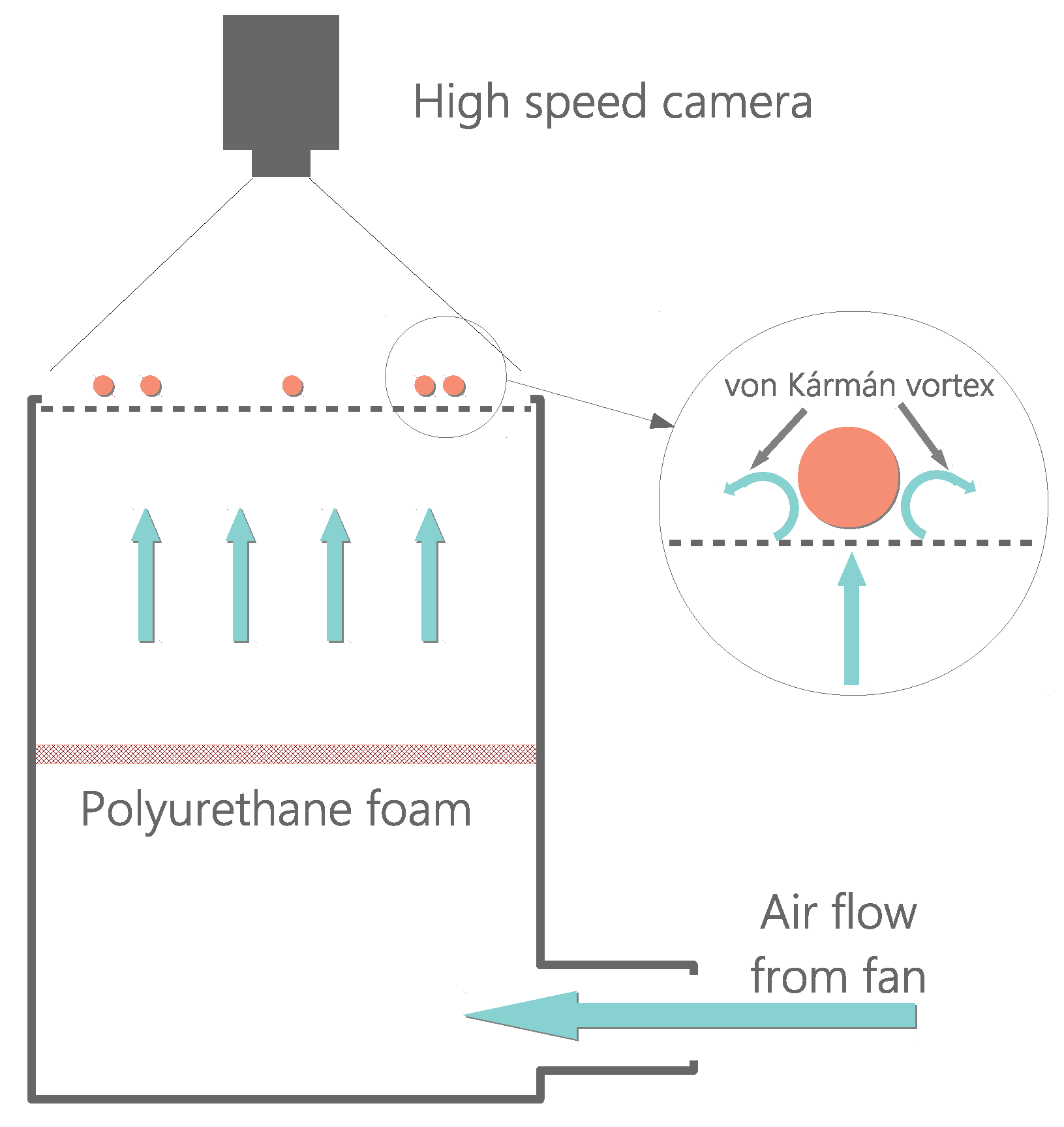
Abstract
1. Introduction
2. Description of the Experiments
2.1. Setup
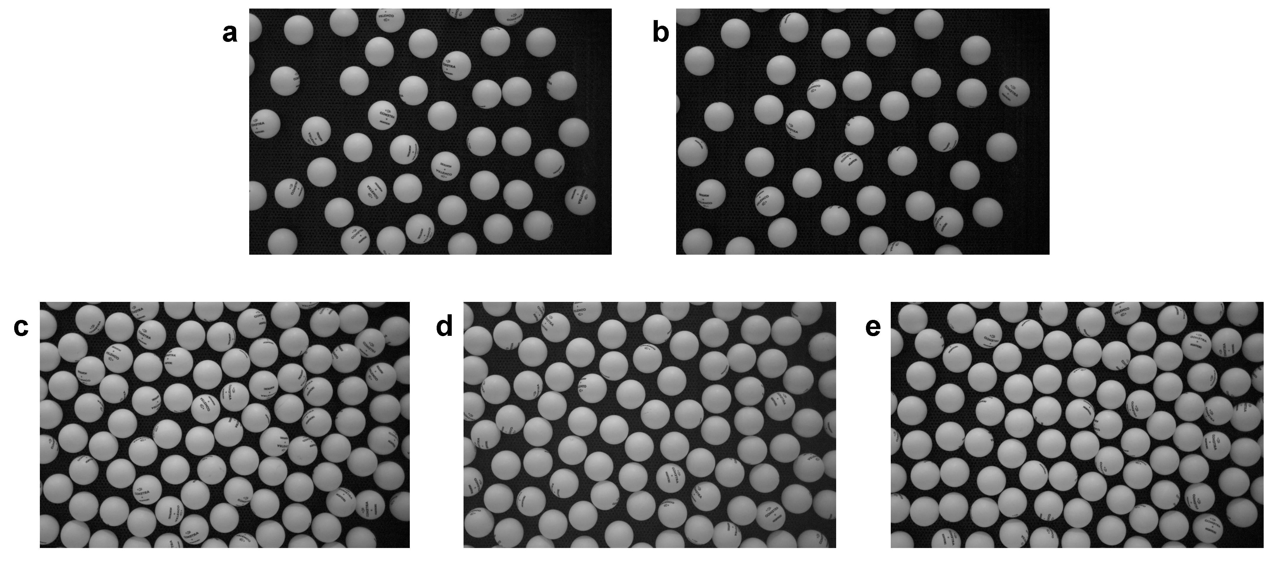
2.2. Phase Behavior
3. Results
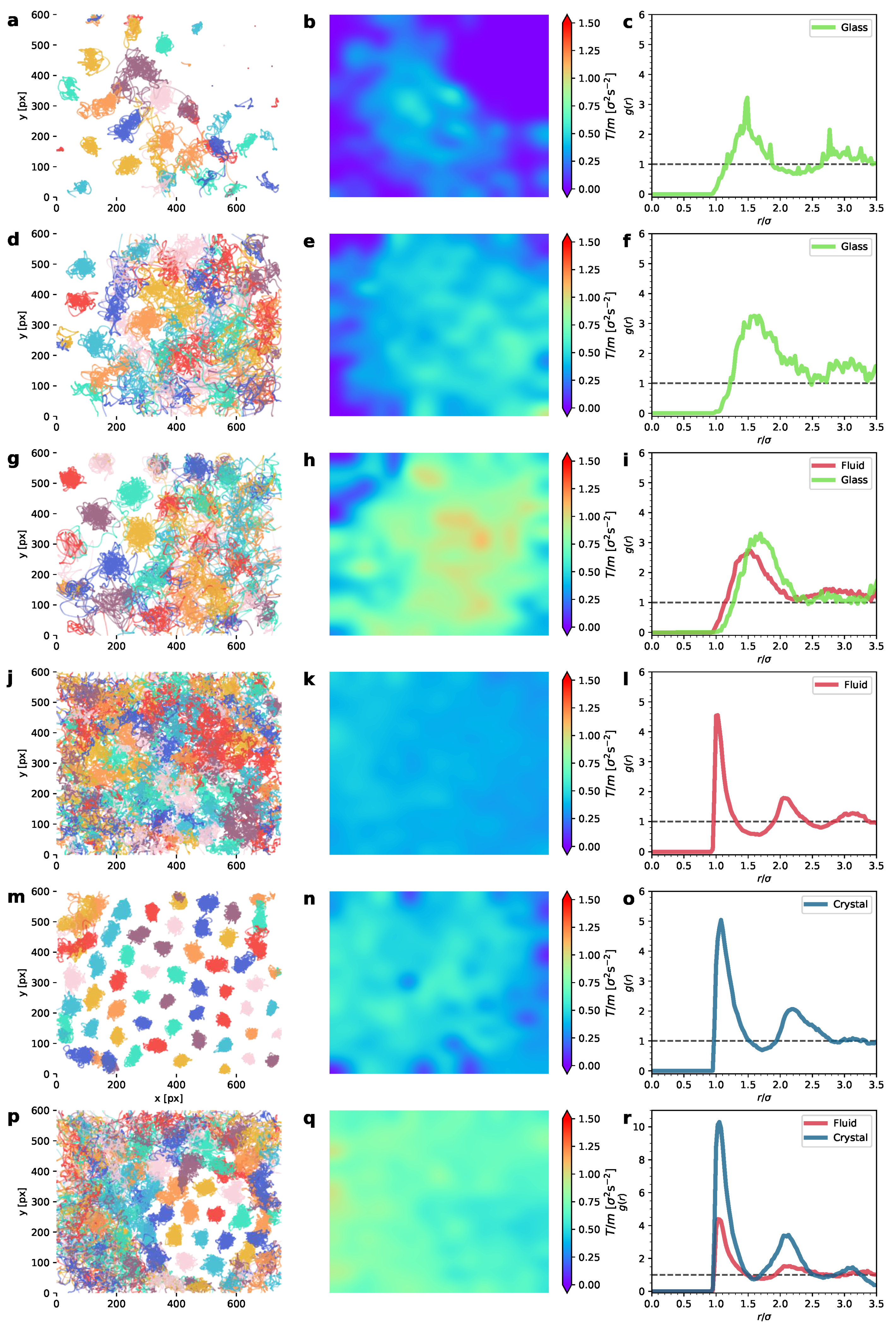
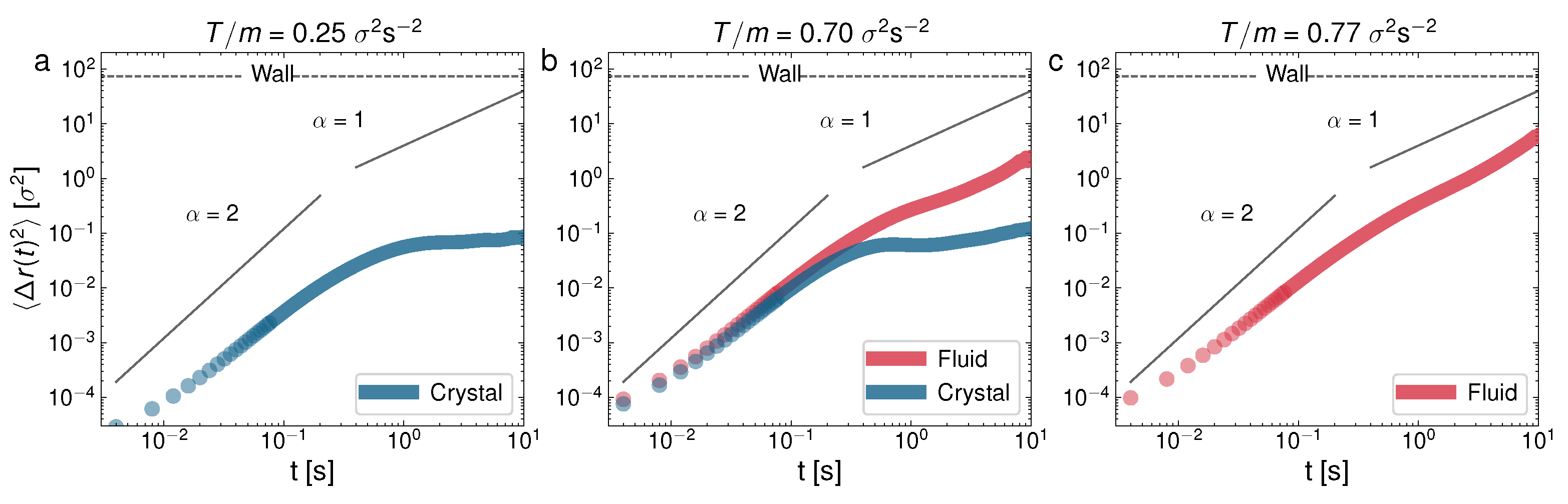
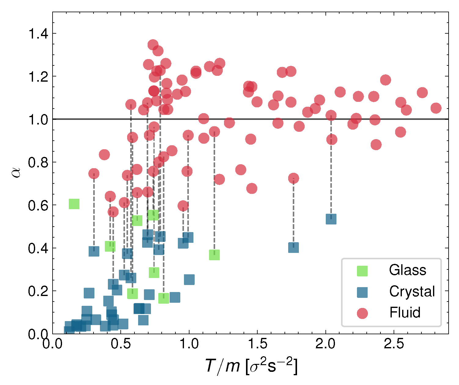
3.1. Trajectories and Granular Temperature Field
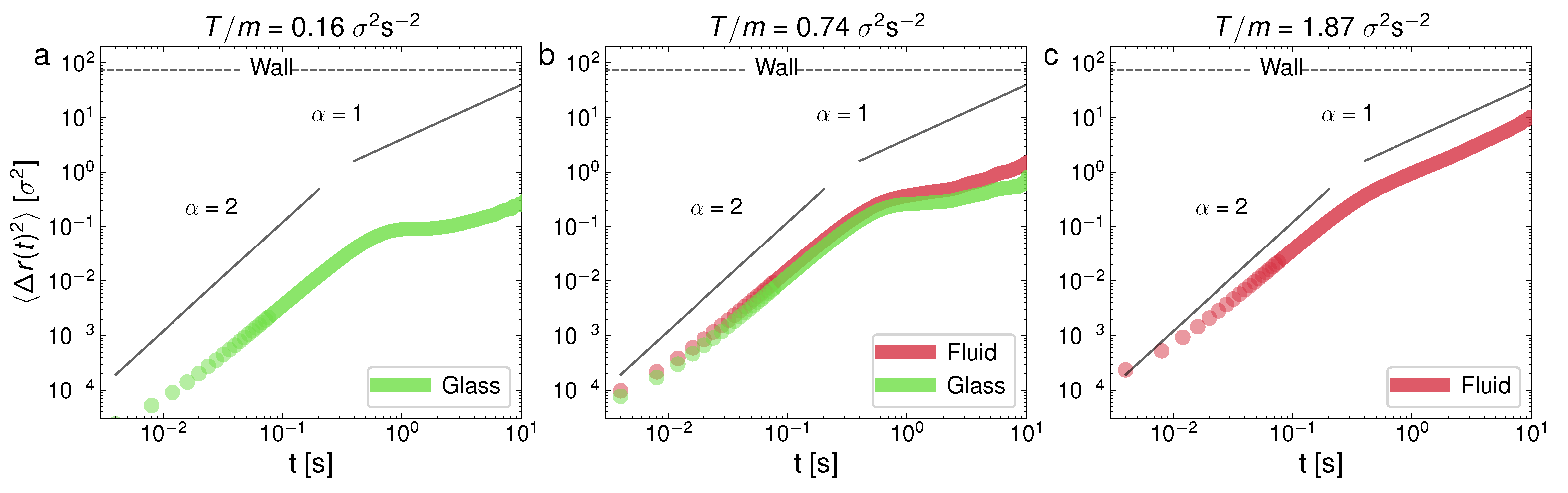
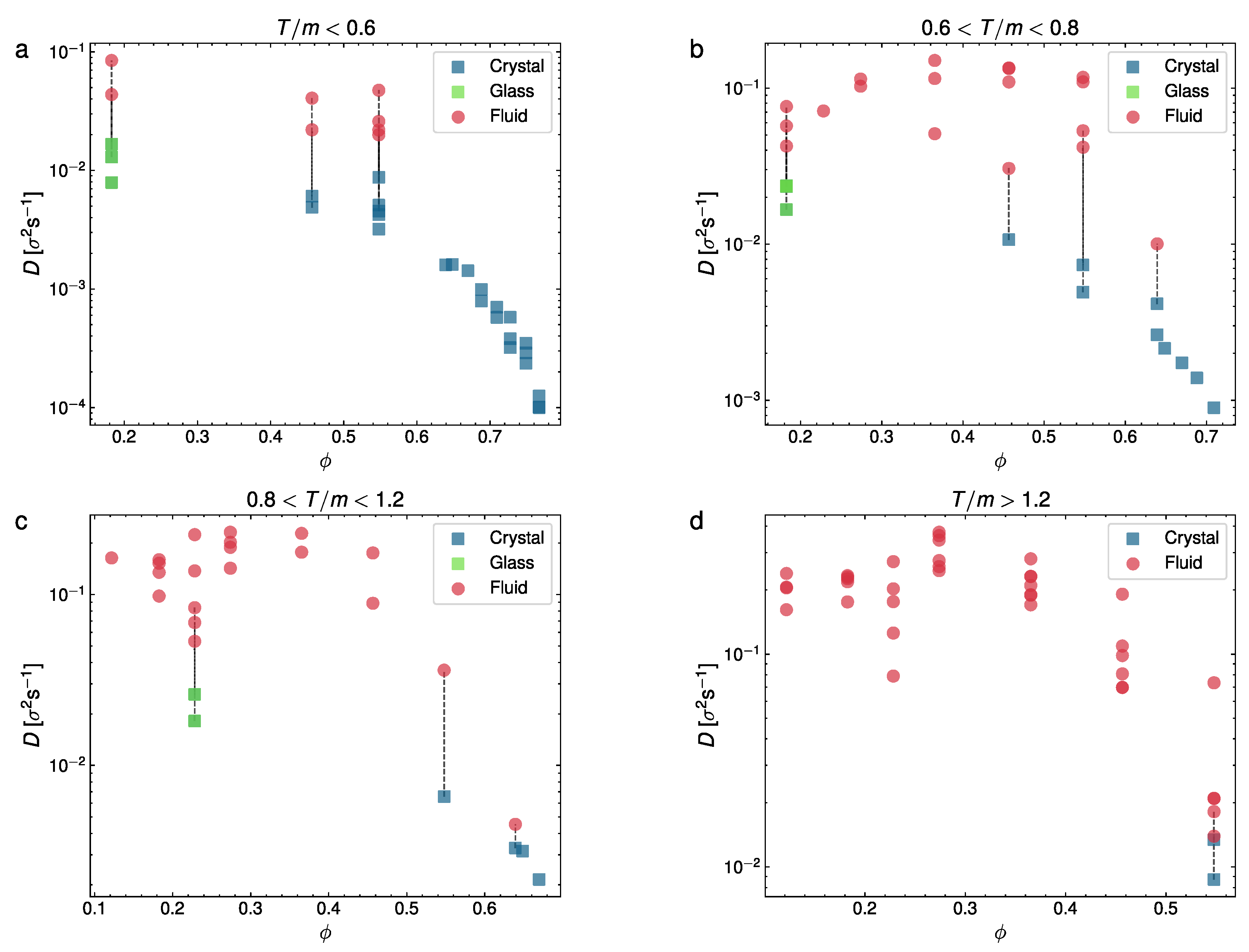
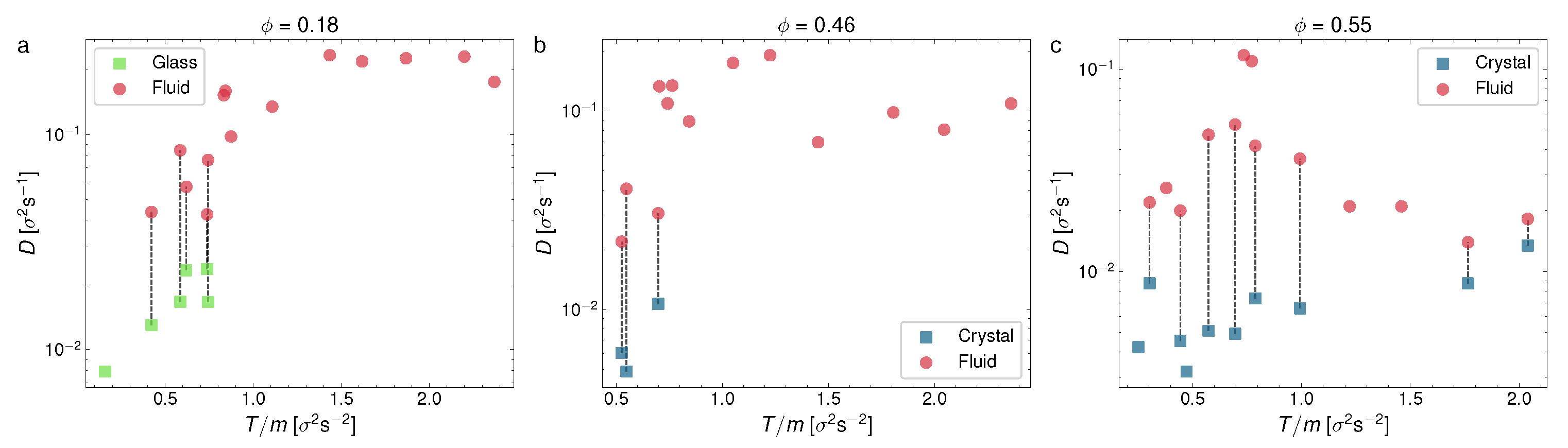
3.2. Diffusion Coefficient
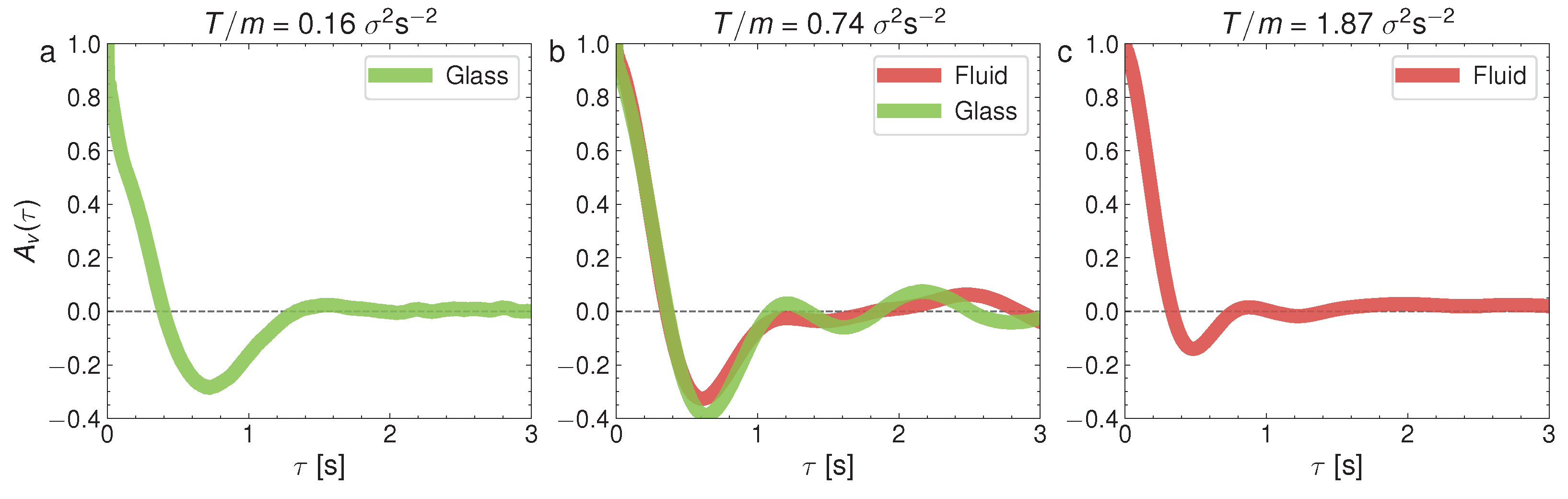
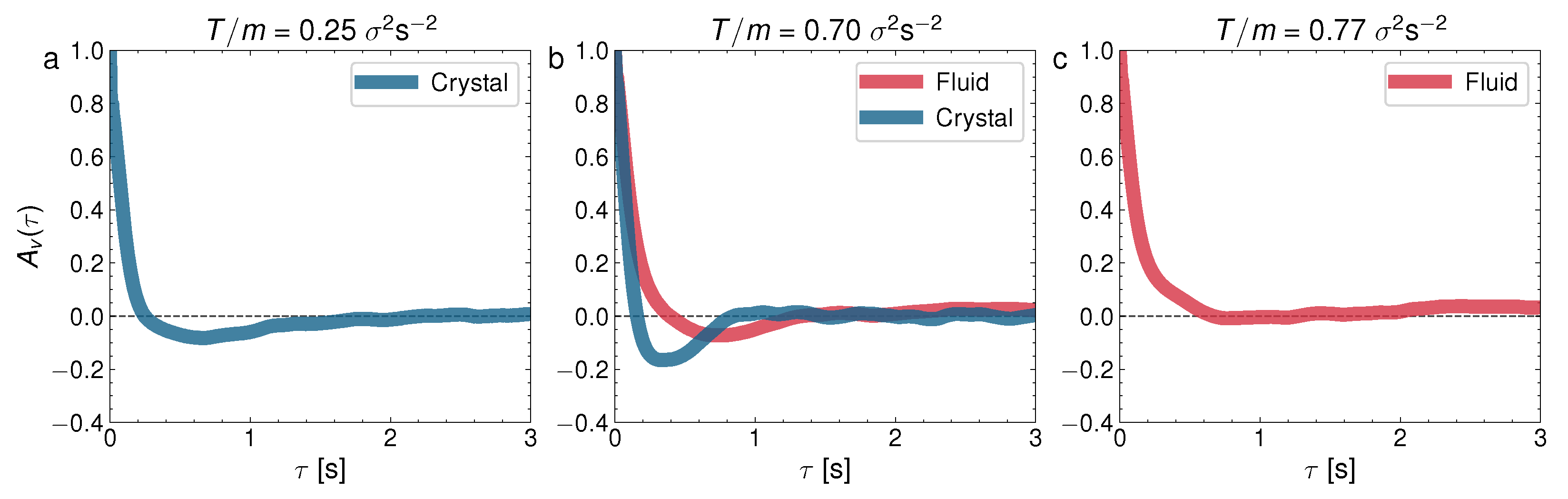
3.3. Velocity Autocorrelations
4. Discussion
Supplementary Materials
Author Contributions
Funding
Data Availability Statement
Acknowledgments
Conflicts of Interest
References
- Jaeger, H.M.; Nagel, S.; Behringer, R. The physics of granular materials. Phys. Today 1996, 49, 32. [Google Scholar] [CrossRef]
- De Gennes, P.G. Granular matter: A tentative view. Rev. Mod. Phys. 1999, 71, S374–S382. [Google Scholar] [CrossRef]
- Aranson, I.S.; Tsimring, L.S. Patterns and collective behavior in granular media: Theoretical concepts. Rev. Mod. Phys. 2006, 78, 641–692. [Google Scholar] [CrossRef]
- Olafsen, J.S.; Urbach, J.S. Clustering, order and collapse in a driven granular monolayer. Phys. Rev. Lett. 1998, 81, 4369–4372. [Google Scholar] [CrossRef]
- Goldhirsch, I. Rapid Granular Flows. Annu. Rev. Fluid Mech. 2003, 35, 267–293. [Google Scholar] [CrossRef]
- Vega Reyes, F.; Urbach, J.S. Steady base states for Navier-Stokes granular hydrolodynamics with boundary heating and shear. J. Fluid Mech. 2009, 636, 279. [Google Scholar] [CrossRef]
- Gantzounis, G.; Yang, J.; Kevrekidis, P.G.; Daraio, C. Granular acoustic switches and logic elements. Nat. Commun. 2014, 5, 5311. [Google Scholar] [CrossRef]
- González-Saavedra, J.F.; Rodríguez-Rivas, Á.; López-Castaño, M.A.; Vega Reyes, F. Acoustic Resonances in a Confined Set of Disks. In Traffic and Granular Flow 2019; Zuriguel, I., Garcimartin, A., Cruz, R., Eds.; Springer International Publishing: Cham, Switzerland, 2020; pp. 349–355. [Google Scholar]
- Mujica, N.; Soto, R. Dynamics of Noncohesive Confined Granular Media. In Recent Advances in Fluid Dynamics with Environmental Applications; Klapp, J., Sigalotti, L.D.G., Medina, A., López, A., Ruiz-Chavarría, G., Eds.; Springer International Publishing: Cham, Switzerland, 2016; pp. 445–463. [Google Scholar]
- Zik, O.; Stavans, J. Self-Diffusion in Granular Flows. Europhys. Lett. (EPL) 1991, 16, 255–258. [Google Scholar] [CrossRef]
- Oger, L.; Annic, C.; Bideau, D.; Dai, R.; Savage, S.B. Diffusion of two-dimensional particles on an air table. J. Stat. Phys. 1996, 82, 1047. [Google Scholar] [CrossRef]
- Ojha, R.P.; Lemieux, P.A.; Dixon, P.K.; Liu, A.J.; Durian, D.J. Statistical mechanics of a gas-fluidized particle. Nature 2004, 427, 521. [Google Scholar] [CrossRef]
- Rosato, A.; Strandburg, K.J.; Prinz, F.; Swendsen, R.H. Why the Brazil nuts are on top: Size segregation of particulate matter by shaking. Phys. Rev. Lett. 1987, 58, 1038–1040. [Google Scholar] [CrossRef] [PubMed]
- Kondic, L.; Hartley, R.R.; Tennakoon, S.G.K.; Painter, B.; Behringer, R.P. Segregation by friction. EPL 2003, 61, 742. [Google Scholar] [CrossRef]
- Jenkins, J.T.; Yoon, D.K. Segregation in Binary Mixtures under Gravity. Phys. Rev. Lett. 2002, 88, 194301. [Google Scholar] [CrossRef] [PubMed]
- Hill, K.M.; Khakhar, D.V.; Gilchrist, J.F.; McCarthy, J.J.; Ottino, J.M. Segregation-driven organization in chaotic granular flows. Proc. Natl. Acad. Sci. 1999, 96, 11701–11706. [Google Scholar] [CrossRef] [PubMed]
- Melby, P.; Vega Reyes, F.; Prevost, A.; Robertson, R.; Kumar, P.; Egolf, D.A.; Urbach, J.S. The dynamics of thin vibrated granular layers. J. Phys. Condens. Matter 2005, 17, S2369. [Google Scholar] [CrossRef]
- Eshuis, P.; van der Weele, K.; van der Meer, D.; Bos, R.; Lohse, D. Phase diagram of vertically shaken granular matter. Phys. Fluids 2007, 19, 123301. [Google Scholar] [CrossRef]
- McLaren, C.P.; Kovar, T.M.; Penn, A.; Müller, C.R.; Boyce, C.M. Gravitational instabilities in binary granular materials. Proc. Natl. Acad. Sci. USA 2019, 116, 9263–9268. [Google Scholar] [CrossRef]
- He, X.; Meerson, B.; Doolen, G. Hydrodynamics of thermal granular convection. Phys. Rev. E 2002, 65, 030301. [Google Scholar] [CrossRef]
- Pontuale, G.; Gnoli, A.; Puglisi, A.; Vega Reyes, F. Thermal Convection in Granular Gases with Dissipative Lateral Walls. Phys. Rev. Lett. 2017, 117, 098006. [Google Scholar] [CrossRef]
- Isobe, M. Statistical law of turbulence in granular gas. J. Phys. Conf. Ser. 2012, 402, 012041. [Google Scholar] [CrossRef]
- Isobe, M. Velocity statistics in two-dimensional granular turbulence. Phys. Rev. E 2003, 68, 040301(R). [Google Scholar] [CrossRef]
- Liu, A.; Nagel, S. Jamming is not just cool anymore. Nature 1998, 396, 21–22. [Google Scholar] [CrossRef]
- Daniels, L.J.; Haxton, T.K.; Xu, N.; Liu, A.J.; Durian, D.J. Temperature-pressure scaling for air-fluidized grains near jamming. Phys. Rev. Lett. 2012, 108, 138001. [Google Scholar] [CrossRef] [PubMed]
- Lasanta, A.; Vega Reyes, F.; Prados, A.; Santos, A. When the Hotter Cools More Quickly: Mpemba Effect in Granular Fluids. Phys. Rev. Lett. 2017, 119, 148001. [Google Scholar] [CrossRef] [PubMed]
- Keim, N.C.; Paulsen, J.D.; Zeravcic, Z.; Sastry, S.; Nagel, S.R. Memory formation in matter. Rev. Mod. Phys. 2019, 91, 035002. [Google Scholar] [CrossRef]
- Prevost, A.; Melby, P.; Egolf, D.A.; Urbach, J.S. Nonequilibrium two-phase coexistence in a confined granular layer. Phys. Rev. E 2004, 70, 050301. [Google Scholar] [CrossRef]
- Reis, P.M.; Ingale, R.A.; Shattuck, M. Crystallization of a quasi-two-dimensional granular fluid. Phys. Rev. Lett. 2006, 96, 258001. [Google Scholar] [CrossRef]
- Vega Reyes, F.; Urbach, J.S. Effect of inelasticity on the phase transitions of a thin vibrated granular layer. Phys. Rev. E 2008, 78, 051301. [Google Scholar] [CrossRef]
- Castillo, G.; Mujica, N.; Soto, R. Criticality of a Granular Solid-Liquid-Like Phase Transi- tion. Phys. Rev. Lett. 2012, 109, 095701. [Google Scholar] [CrossRef]
- Néel, B.; Rondini, I.; Turzillo, A.; Mujica, N.; Soto, R. Dynamics of a first-order transition to an absorbing state. Phys. Rev. E 2014, 89, 042206. [Google Scholar] [CrossRef]
- Non-Gaussian velocity distributions in excited granular matter in the absence of clustering. Phys. Rev. E 2000, 62, R1489–R1492. [CrossRef] [PubMed]
- González-Pinto, M.; Borondo, F.; Martínez-Ratón, Y.; Velasco, E. Clustering in vibrated monolayers of granular rods. Soft Matter 2017, 13, 2571. [Google Scholar] [CrossRef] [PubMed]
- Olafsen, J.S.; Urbach, J.S. Two-Dimensional Melting Far from Equilibrium in a Granular Monolayer. Phys. Rev. Lett. 2005, 95, 098002. [Google Scholar] [CrossRef] [PubMed]
- Castillo, G.; Mujica, N.; Soto, R. Universality and criticality of a second-order granular solid-liquid-like phase transition. Phys. Rev. E 2015, 91, 012141. [Google Scholar] [CrossRef] [PubMed]
- Vega Reyes, F.; Santos, A.; Garzó, V. Non-Newtonian Granular Hydrodynamics. What Do the Inelastic Simple Shear Flow and the Elastic Fourier Flow Have in Common? Phys. Rev. Lett. 2010, 104, 028001. [Google Scholar] [CrossRef] [PubMed]
- Rietz, F.; Radin, C.; Swinney, H.L.; Schröter, M. Nucleation in Sheared Granular Matter. Phys. Rev. Lett. 2018, 120, 055701. [Google Scholar] [CrossRef]
- Goldhirsch, I.; Zanetti, G. Clustering instability in dissipative gases. Phys. Rev. Lett. 1993, 70, 1619–1622. [Google Scholar] [CrossRef]
- Prevost, A.; Egolf, D.A.; Urbach, J.S. Forcing and Velocity Correlations in a Vibrated Granular Monolayer. Phys. Rev. Lett. 2002, 89, 084301. [Google Scholar] [CrossRef]
- Kosterlitz, J.M.; Thouless, D.J. Long range order and metastability in two dimensional solids and superfluids. (Application of dislocation theory). J. Phys. C 1972, 5, L124–L126. [Google Scholar] [CrossRef]
- Kosterlitz, J.M.; Thouless, D.J. Ordering, metastability and phase transitions in two-dimensional systems. J. Phys. C 1973, 6, 1181. [Google Scholar] [CrossRef]
- Nelson, D.R.; Halperin, B.I. Dislocation mediated melting in two dimensions. Phys. Rev. B 1979, 19, 2457. [Google Scholar] [CrossRef]
- Young, A.P. Melting and the vector Coulomb gas in two dimensions. Phys. Rev. B 1979, 19, 1855. [Google Scholar] [CrossRef]
- Strandburg, K.J. Two-dimensional melting. Rev. Mod. Phys. 1988, 60, 161. [Google Scholar] [CrossRef]
- Komatsu, Y.; Tanaka, H. Roles of Energy Dissipation in a Liquid-Solid Transition of Out-of-Equilibrium Systems. Phys. Rev. X 2015, 5, 031025. [Google Scholar] [CrossRef]
- Foerster, S.F.; Louge, M.Y.; Chang, H.; Allia, K. Measurements of the collision properties of small spheres. Phys. Fluids 1994, 6, 1108–1115. [Google Scholar] [CrossRef]
- Olafsen, J.S.; Urbach, J.S. Velocity distributions and density fluctuations in a granular gas. Phys. Rev. E 1999, 60, R2468. [Google Scholar] [CrossRef] [PubMed]
- Olafsen, J.S.; Urbach, J.S. Experimental observations of non-equilibrium distributions and transitions in a 2D granular gas. In Granular Gases; Springer: Berlin, Germany, 2001; Volume Lecture Notes in Physics, pp. 410–428. [Google Scholar]
- Brey, J.J.; Dufty, J.W.; Kim, C.S.; Santos, A. Hydrodynamics for granular flow at low density. Phys. Rev. E 1998, 58, 4638–4653. [Google Scholar] [CrossRef]
- Brey, J.J.; Cubero, D. Hydrodynamic transport coefficients of granular gases. In Granular Gases; Springer: Berlin, Germany, 2001; Volume Lecture Notes in Physics, pp. 59–78. [Google Scholar]
- Bechinger, C.; Di Leonardo, R.; Löwen, H.; Reichhardt, C.; Volpe, G.; Volpe, G. Active particles in complex and crowded environments. Rev. Mod. Phys. 2016, 88, 045006. [Google Scholar] [CrossRef]
- Digregorio, P.; Levis, D.; Suma, A.; Cugliandolo, L.F.; Gonnella, G.; Pagonabarraga, I. Full Phase Diagram of Active Brownian Disks: From Melting to Motility-Induced Phase Separation. Phys. Rev. Lett. 2018, 121, 098003. [Google Scholar] [CrossRef]
- Ojha, R.P.; Abate, A.R.; Durian, D.J. Statistical characterization of the forces on spheres in an upflow of air. Phys. Rev. E 2005, 71, 016313. [Google Scholar] [CrossRef]
- Batchelor, G.K. Transport properties of two-phase materials with random structure. Ann. Rev. Fluid Mech. 1974, 6, 227–255. [Google Scholar] [CrossRef]
- López-Castaño, M.A.; González-Saavedra, J.F.; Rodríguez-Rivas, A.; Abad, E.; Yuste, S.B.; Vega Reyes, F. Pseudo-two-dimensional dynamics in a system of macroscopic rolling spheres. Phys. Rev. E 2021, 103, 042903. [Google Scholar] [CrossRef] [PubMed]
- Abate, A.R.; Durian, D.J. Partition of energy for air-fluidized grains. Phys. Rev. E 2005, 72, 031305. [Google Scholar] [CrossRef] [PubMed]
- López-Castaño, M.A.; González-Saavedra, J.F.; Rodríguez-Rivas, Á.; Vega Reyes, F. Statistical Properties of a Granular Gas Fluidized by Turbulent Air Wakes. In Traffic and Granular Flow 2019; Zuriguel, I., Garcimartin, A., Cruz, R., Eds.; Springer International Publishing: Cham, Switzerland, 2020; pp. 397–403. [Google Scholar]
- Koyama, S.; Matsuno, T.; Noguchi, T. Anomalous diffusion in a monolayer of lightweight spheres fluidized in air flow. Phys. Rev. E 2021, 104, 054901. [Google Scholar] [CrossRef]
- Maw, N.; Barber, J.R.; Fawcett, J.N. The Role of Elastic Tangential Compliance in Oblique Impact. J. Lubr. Technol. 1981, 103, 74–80. [Google Scholar] [CrossRef]
- Taneda, S. Visual observations of the flow past a sphere at Reynolds numbers between 104 and 106. J. Fluid Mech. 1978, 85, 187–192. [Google Scholar] [CrossRef]
- Van Dyke, M. An Album of Fluid Motion; The Parabolic Press: Stanford, CA, USA, 1982. [Google Scholar]
- Montanero, J.M.; Garzó, V.; Santos, A.; Brey, J.J. Kinetic theory of simple granular shear flows of smooth hard spheres. J. Fluid Mech. 1999, 389, 391–411. [Google Scholar] [CrossRef]
- OpenCV. Available online: https://opencv.org/ (accessed on 10 November 2022).
- Allan, D.B.; Caswell, T.; Keim, N.C.; van der Wel, C.M. Soft-Matter/Trackpy: Trackpy v0.4.2. 2019. Available online: https://soft-matter.github.io/trackpy/v0.5.0/ (accessed on 10 November 2022).
- Vega Reyes, F.; Rodríguez-Rivas, A.; González-Saavedra; López-Castaño, M.A. Available online: https://github.com/fvegar/Tracks (accessed on 10 November 2022).
- Kanatani, K.I. A micropolar continuum theory for the flow of granular materials. Int. J. Engng. Sci. 1979, 17, 419–432. [Google Scholar] [CrossRef]
- Desmond, K.W.; Weeks, E.R. Random close packing of disks and spheres in confined geometries. Phys. Rev.-Stat. Nonlinear Soft Matter Phys. 2009, 80, 051305. [Google Scholar] [CrossRef]
- Rodríguez-Rivas, A.; Romero-Enrique, J.M.; Rull, L.F. Molecular simulation study of the glass transition in a soft primitive model for ionic liquids. Mol. Phys. 2019, 117, 3941–3956. [Google Scholar] [CrossRef]
- Metzler, R.; Jeon, J.H.; Cherstvy, A.G.; Barkai, E. Anomalous diffusion models and their properties: Non-stationarity, non-ergodicity, and ageing at the centenary of single particle tracking. Phys. Chem. Chem. Phys. 2014, 16, 24128–24164. [Google Scholar] [CrossRef] [PubMed]
- Kranz, W.T.; Sperl, M.; Zippelius, A. Glass Transition for Driven Granular Fluids. Phys. Rev. Lett. 2010, 104. [Google Scholar] [CrossRef] [PubMed]
- Vega Reyes, F.; López-Castaño, M.A.; Rodríguez-Rivas, A. Diffusive regimes in a two-dimensional chiral fluid. Commun. Phys. 2022, 5, 1–7. [Google Scholar] [CrossRef]


Publisher’s Note: MDPI stays neutral with regard to jurisdictional claims in published maps and institutional affiliations. |
© 2022 by the authors. Licensee MDPI, Basel, Switzerland. This article is an open access article distributed under the terms and conditions of the Creative Commons Attribution (CC BY) license (https://creativecommons.org/licenses/by/4.0/).
Share and Cite
Vega Reyes, F.; Rodríguez-Rivas, Á.; González-Saavedra, J.F.; López-Castaño, M.A. Diffusion and Velocity Correlations of the Phase Transitions in a System of Macroscopic Rolling Spheres. Entropy 2022, 24, 1684. https://doi.org/10.3390/e24111684
Vega Reyes F, Rodríguez-Rivas Á, González-Saavedra JF, López-Castaño MA. Diffusion and Velocity Correlations of the Phase Transitions in a System of Macroscopic Rolling Spheres. Entropy. 2022; 24(11):1684. https://doi.org/10.3390/e24111684
Chicago/Turabian StyleVega Reyes, Francisco, Álvaro Rodríguez-Rivas, Juan F. González-Saavedra, and Miguel A. López-Castaño. 2022. "Diffusion and Velocity Correlations of the Phase Transitions in a System of Macroscopic Rolling Spheres" Entropy 24, no. 11: 1684. https://doi.org/10.3390/e24111684
APA StyleVega Reyes, F., Rodríguez-Rivas, Á., González-Saavedra, J. F., & López-Castaño, M. A. (2022). Diffusion and Velocity Correlations of the Phase Transitions in a System of Macroscopic Rolling Spheres. Entropy, 24(11), 1684. https://doi.org/10.3390/e24111684