
Performance Modulation of S-CO2 Brayton Cycle for Marine Low-Speed Diesel Engine Flue Gas Waste Heat Recovery Based on MOGA


Abstract
1. Introduction
2. Marine Low-Speed Engine Modeling and Validation
2.1. Marine Low-Speed Diesel Engine Modeling
2.2. The Algorithm Fitting for Marine Low-Speed Diesel Engine Model
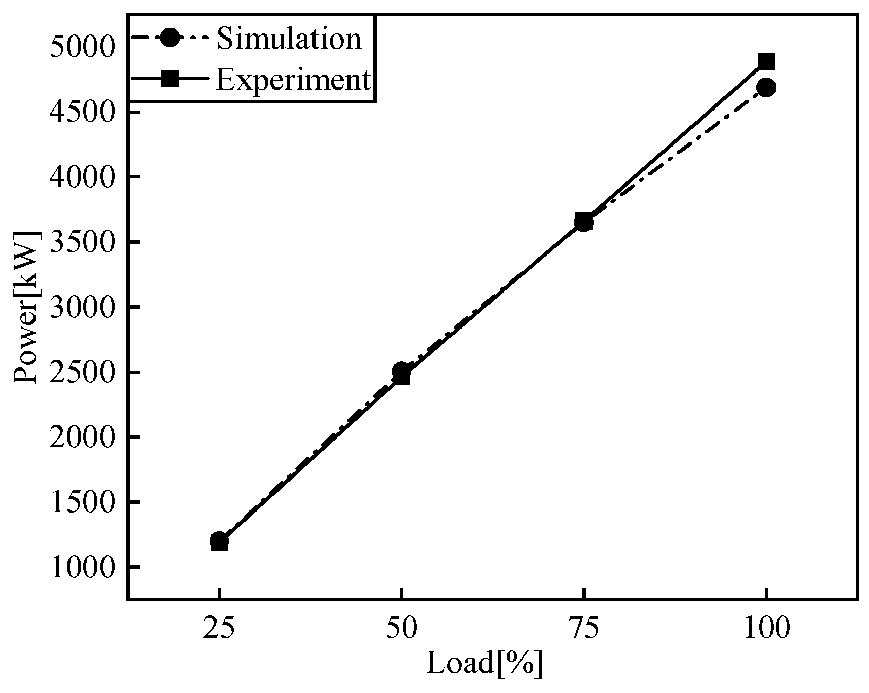
2.3. The Validation of Marine Low-Speed Diesel Engine Model
3. S-CO2 Brayton Cycle Waste Heat Recovery Model
3.1. Flue Gas Waste Heat Recovery Layout
3.2. SCRBC Thermodynamic Model
- The system is in a stable state, and the change in kinetic energy is ignored;
- Isentropic efficiency is adopted for the turbines and compressors;
- Except the cooler, the heat transfer loss of the whole cycle and environment is ignored;
- The effectiveness of HTR and LTR are considered;
- The end difference at the cooler, regenerator and heat exchanger is considered;
- The parameters of each state point do not change with time. The thermodynamic model of each component of the cycle is shown in Table 4.
3.3. Matching of WHR Parameters for Multiple Operating Conditions
4. Timing Adjustment for Waste Heat Modulation
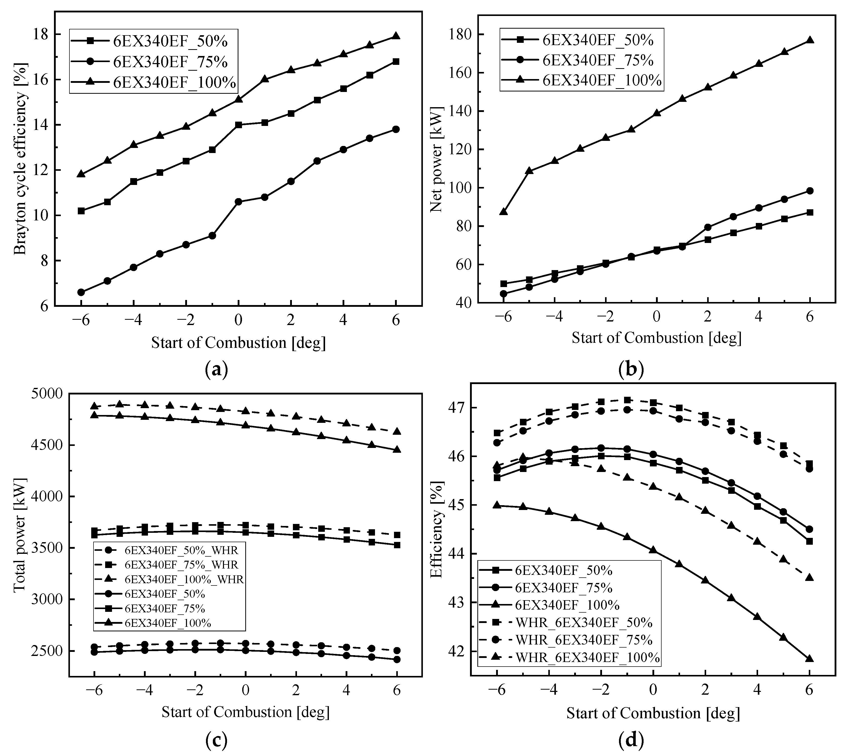
4.1. The Effect of Injection Timing on Residual Heat Modulation
4.2. The Effect of Exhaust Timing on Residual Heat Modulation
5. S-CO2 Waste Heat Recovery Performance Evaluation
5.1. Optimized Timing Modulation Based on MOGA
5.2. Thermodynamic Evaluation
5.3. Emissivity Evaluation
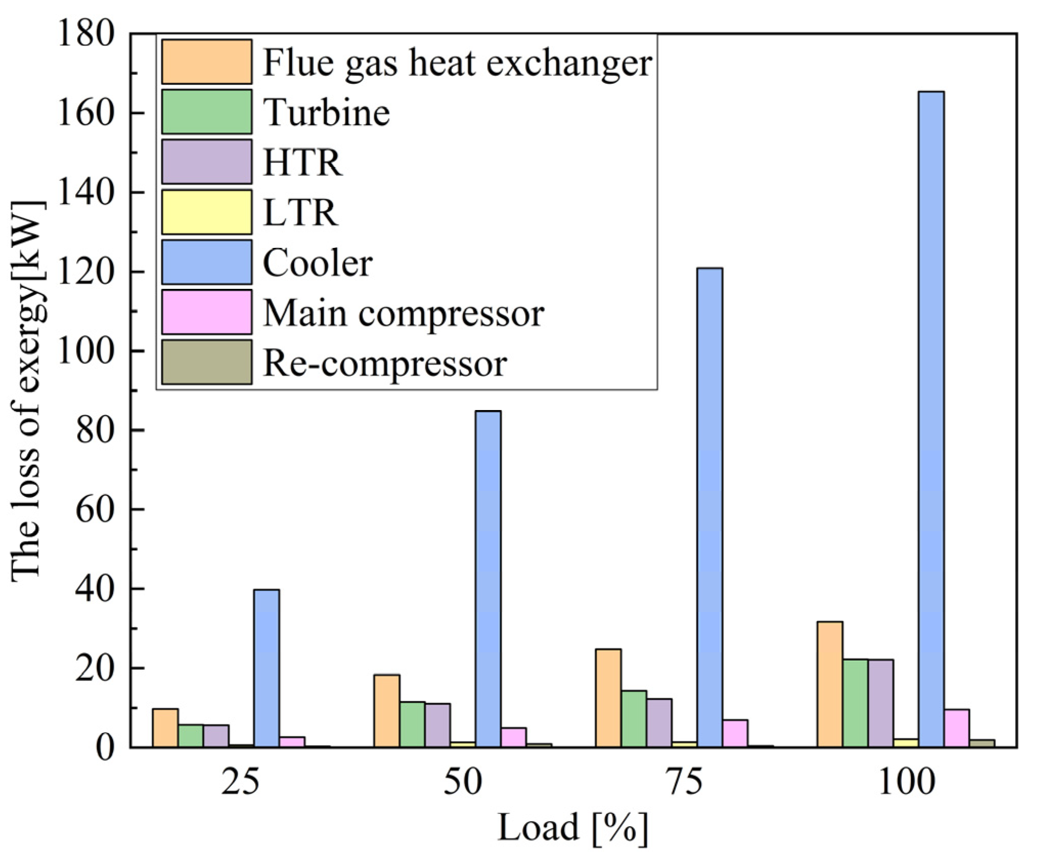
5.4. Exergy Analysis
6. Conclusions
- (1)
- With the structural parameters of 6EX340EF marine low-speed diesel engine, the low-speed engine model was established in AVL Cruise M and verified by the bench test data. The optimum combustion parameters for each load were obtained by fitting the cylinder pressure curve and the ROHR curve with the MOGA algorithm. A one-dimensional simulation model of the S-CO2 recompression Brayton cycle system for the low-speed engine flue gas waste heat recovery was developed in EBSILON, and the accuracy of the model was verified by SANDIA experimental data. On this basis, the effects of injection timing and valve timing parameters on the comprehensive performance of the main engine and the waste heat recovery system were investigated.
- (2)
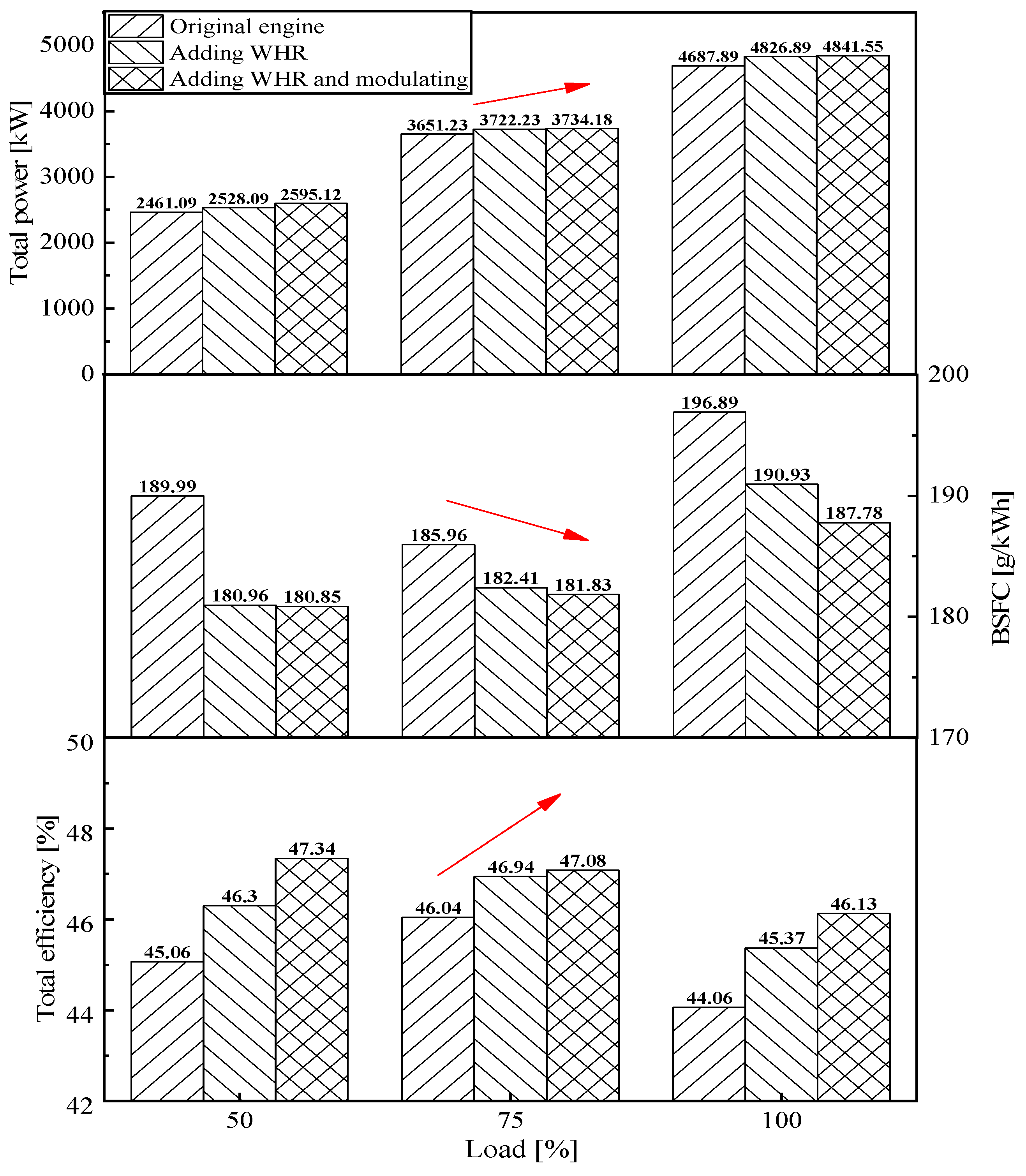
- By optimizing the timing modulation parameters through MOGA and evaluating the flue gas waste heat recovery from the perspective of thermodynamic performance, the research on the performance modulation method of the S-CO2 Brayton cycle for flue gas waste heat in marine low-speed engines has been completed. The SCRBC with waste heat modulation will further increase the total power and efficiency, which in turn brings about a reduction in fuel consumption rate. The efficiency of the SCRBC system with the addition of waste heat recovery increases by 1.24%, 0.90% and 1.31% at 50%, 75% and 100%, respectively, while the efficiency of the SCRBC system with the addition of waste heat modulation increases by 2.28%, 1.04% and 2.07% at 50%, 75% and 100%, respectively. The SCRBC system with the waste heat modulation had annual CO2 emission reductions for each load of the low-speed engine, and the maximum annual CO2 emission reduction of 748.51 × 10³ kg·a−1 occurred at 50% load.
- (3)
- With the exergy analysis, the cooler has the largest system exergy loss of 165 kW, with the exergy loss efficiency of 2.06% under 100% load. The second is flue gas heat exchanger with the exergy loss of 165 kW, and the exergy loss efficiency of 2.06%. Further optimization of the SCRBC system should first focus on improving these two components.
- (4)
- The evaluation of the low-speed engine flue gas waste heat recovery from the perspective of thermodynamic performance and energy saving and emission reduction efficiency was carried out. The research on the performance modulation method of S-CO2 Brayton cycle for flue gas waste heat in marine low-speed engine has been completed, which further improves the efficiency of the system and can be extended to other engines.
Author Contributions
Funding
Institutional Review Board Statement
Informed Consent Statement
Data Availability Statement
Conflicts of Interest
Nomenclature
| Abbreviations | |
| IMO | International Maritime Organization |
| WHR | Waste Heat Recovery |
| EEDI | Energy Efficiency Design Index |
| PT | Power Turbine |
| ET | Electrical Turbine |
| TEG | Thermoelectric Generator |
| ORC | Organic Rankine Cycle |
| SCBC | Supercritical Carbon Dioxide Brayton Cycle |
| S-CO2 | Supercritical Carbon Dioxide |
| SCRBC | S-CO2 Recompression Brayton Cycle |
| MOGA | Multi-objective Genetic Algorithm |
| HPCR | High-Pressure Common Rail |
| ROHR | Rate of Heat Release |
| LTR | Low-Temperature Recuperator |
| HTR | High-Temperature Recuperator |
| BSFC | Brake Specific Fuel Consumption |
| CA | Crank Angle |
| RSM | Response Surface Methodology |
| Subscripts and superscripts | |
| T | Turbine |
| MC | Main Compressor |
| RC | Re-compressor |
| Heater | Heat Exchanger |
| Cooler | Cooler |
| LTR | Low-Temperature Recuperator |
| HTR | High-Temperature Recuperator |
| fuel | Diesel Fuel |
| X+ | The Supplying Exergy |
| X− | The Effective Exergy |
| X,L | The Total Exergy Loss |
| exe | Exergy |
| xlf | Exergy Loss of Flue Gas Heat Exchanger |
| xlt | Exergy Loss of Turbine |
| xlh | Exergy Loss of HTR |
| xll | Exergy Loss of LTR |
| xlc | Exergy Loss of Cooler |
| xlmc | Exergy Loss of Main Compressor |
| xlrc | Exergy Loss of Re-compressor |
| xls | Exergy Loss of Splitter |
| xlm | Exergy Loss of Mixer |
| 1, …8 | Thermodynamic State Points (Figure 9) |
| Symbols | |
| P | Pressure (MPa) |
| E | Specific exergy (kJ/kg) |
| q | Thermal energy (kW) |
| S | Entropy (kJ/(kg·K)) |
| T | Temperature (K or °C) |
| W | Work Down, Power (kW) |
| h | Specific Enthalpy (kJ/kg) |
| η | Efficiency (%) |
| r | Split ratio (-) |
| k | The Slope of (-) |
| CP | Specific Heat Capacity (kJ/(kg·K)) |
| m | Mass Flow Rate (kg/s) |
| κ | Polytropic Coefficient |
| x | The Value of the Factor |
| β | The Regression Coefficient |
| ε | The Error |
| R | Annual CO2 Emission Reduction |
| f | The CO2 Emission Factor |
References
- Nielsen, R.F.; Haglind, F.; Larsen, U. Design and modelling of an advanced marine machinery system including waste heat recovery and removal of Sulphur oxides. Energy Convers. Manag. 2014, 85, 687–693. [Google Scholar] [CrossRef]
- Hossain, S.N.; Bari, S. Waste heat recovery from a diesel engine using shell and tube heat exchanger. Appl. Therm. Eng. 2013, 61, 355–363. [Google Scholar]
- Shi, L.F.; Tian, H.; Shu, G.Q. Multi-mode analysis of a CO2-based combined refrigeration and power cycle for engine waste heat recovery. Appl. Energy 2020, 264, 114670. [Google Scholar] [CrossRef]
- Zhang, R.Y.; Su, W.; Lin, X.X.; Zhou, N.J.; Zhao, L. Thermodynamic analysis and parametric optimization of a novel S–CO2 power cycle for the waste heat recovery of internal combustion engines. Energy 2020, 209, 11848. [Google Scholar] [CrossRef]
- Hountalas, D.T.; Rogdakis, E.D.; Kouremenos, D.A.; Katsanos, C.O. Study of available exhaust gas heat recovery technologies for HD diesel engine applications. Int. J. Altern. Propuls. 2007, 1, 228–249. [Google Scholar] [CrossRef]
- Hopmann, U. Diesel engine waste heat recovery utilizing electric turbo-compound technology. In Proceedings of the Diesel Engine Emissions Reduction (DEER) Conference, San Diego, CA, USA, 29 August–2 September 2004. [Google Scholar]
- Weerasinghe, W.M.; Stobart, R.K.; Hounsham, S.M. Thermal efficiency improvement in high output diesel engines a comparison of a Rankine cycle with turbo-compounding. Appl. Therm. Eng. 2010, 30, 2253–2256. [Google Scholar] [CrossRef]
- Lan, S.; Yang, Z.J.; Chen, R.; Stobart, R. A dynamic model for thermoelectric generator applied to vehicle waste heat recovery. Appl. Energy 2018, 210, 327–338. [Google Scholar] [CrossRef]
- Yang, H.Q.; Shu, G.Q.; Tian, H.; Ma, X.N.; Chen, T.Y.; Liu, P. Optimization of thermoelectric generator (TEG) integrated with three-way catalytic converter (TWC) for harvesting engine’s exhaust waste heat. Appl. Therm. Eng. 2018, 144, 628–638. [Google Scholar] [CrossRef]
- Merve, A.; Hüseyin, Y.; Yıldız, K.; Ali, K.; Ali, S.; Recep, Y. Why Kalina (Ammonia-Water) cycle rather than steam Rankine cycle and pure ammonia cycle: A comparative and comprehensive case study for a cogeneration system. Energy Convers. Manag. 2022, 265, 115739. [Google Scholar]
- Özkan, K.; Yıldız, K.; Hüseyin, Y. Is Kalina cycle or organic Rankine cycle for industrial waste heat recovery applications? A detailed performance, economic and environment based comprehensive analysis. Process Saf. Environ. Prot. 2022, 163, 421–437. [Google Scholar]
- Emrullah, K.; Cuma, K.; Hüseyin, Y.; Yıldız, K.; Recep, Y.; Ali, K. Pinch point determination and Multi-Objective optimization for working parameters of an ORC by using numerical analyses optimization method. Energy Convers. Manag. 2022, 271, 116301. [Google Scholar]
- Song, B.Y.; Zhuge, W.L.; Zhao, R.C.; Zheng, X.Q.; Zhang, Y.J.; Yin, Y.; Zhao, Y.T. An investigation on the performance of a Brayton cycle waste heat recovery system for turbocharged diesel engines. J. Mech. Sci. Technol. 2013, 27, 1721–1729. [Google Scholar] [CrossRef]
- Bian, X.Y.; Wang, X.; Wang, R.; Cai, J.W.; Tian, H.; Shu, G.Q.; Lin, Z.M.; Yu, X.Y.; Shi, L.F. A comprehensive evaluation of the effect of different control valves on the dynamic performance of a recompression supercritical CO2 Brayton cycle. Energy 2022, 248, 123630. [Google Scholar] [CrossRef]
- Feng, Y.M.; Du, Z.Q.; Shreka, M.; Zhu, Y.Q.; Zhou, S.; Zhang, W.P. Thermodynamic analysis and performance optimization of the supercritical carbon dioxide Brayton cycle combined with the Kalina cycle for waste heat recovery from a marine low-speed diesel engine. Energy Convers. Manag. 2020, 206, 112483. [Google Scholar] [CrossRef]
- Miller, J.D.; Buckmaster, D.J.; Hart, K.; Held, T.J.; Thimsen, D.; Maxson, A.; Phillips, J.N.; Hume, S. Comparison of Supercritical CO2 Power Cycles to Steam Rankine Cycles in Coal-Fired Applications. In Proceedings of the ASME Turbo Expo 2017: Turbomachinery Technical Conference and Exposition, Charlotte, NC, USA, 26–30 June 2017. [Google Scholar]
- Gao, Y. Simulation and Optimization of the Performance of Marine Main Diesel Engine in Waste Heat Utilization System. Ph.D. Thesis, Harbin Engineering University, Harbin, China, 2013. [Google Scholar]
- Wang, Q.P.; Li, J.; Yang, J.G.; Yu, Y.H. Research on Real-Time Simulation Model for Electronically Controlled Low-Speed Marine Diesel Engine. Chin. Intern. Combust. Engine Eng. 2021, 42, 60–67, 75. [Google Scholar]
- Pan, M.Z.; Zhu, Y.; Bian, X.Y.; Liang, Y.C.; Lu, F.L. Theoretical analysis and comparison on supercritical CO2 based combined cycles for waste heat recovery of engine. Energy Convers. Manag. 2020, 219, 113049. [Google Scholar] [CrossRef]
- Siddiqui, M.E.; Almitani, K.H. Proposal and Thermodynamic Assessment of S-CO2 Brayton Cycle Layout for Improved Heat Recovery. Entropy 2020, 22, 305. [Google Scholar] [CrossRef] [PubMed]
- Hu, N.; Zhou, P.L.; Yang, J.G. Comparison and combination of NLPQL and MOGA algorithms for a marine medium-speed diesel engine optimization. Energy Convers. Manag. 2017, 133, 138–152. [Google Scholar] [CrossRef]
- Wang, K.; Li, M.J.; Guo, J.Q.; Li, P.W.; Liu, Z.B. A systematic comparison of different S-CO2 Brayton cycle layouts based on multi-objective optimization for applications in solar power tower plants. Appl. Energy 2018, 212, 109–121. [Google Scholar] [CrossRef]
- Xie, L.T.; Yang, J.G.; Dong, F. Optimization of S-CO2 Brayton cycle system for flue gas waste heat of marine low-speed diesel engine. J. Dalian Marit. Univ. 2022, 48, 89–97. [Google Scholar]
- Liu, C.; Yang, Q.G.; Cui, G.M. Supercritical Carbon Dioxide(s-CO2) Power Cycle for Waste Heat Recovery: A Review from Thermodynamic Perspective. Processes 2020, 8, 1461. [Google Scholar] [CrossRef]
- Yu, A.F.; Su, W.; Lin, X.X.; Zhou, L. Thermodynamic analysis on the combination of supercritical carbon dioxide power cycle and transcritical carbon dioxide refrigeration cycle for the waste heat recovery of shipboard. Energy Convers. Manag. 2020, 221, 113214. [Google Scholar] [CrossRef]
- Cheng, W.-L.; Huang, W.-X.; Nian, Y.-L. Global parameter optimization and criterion formula of supercritical carbon dioxide Brayton cycle with recompression. Energy Convers. Manag. 2017, 150, 669–677. [Google Scholar] [CrossRef]
- Son, S.M.; Heo, J.Y.; Lee, J.I. Prediction of inner pinch for supercritical CO2 heat exchanger using Artificial Neural Network and evaluation of its impact on cycle design. Energy Convers. Manag. 2018, 163, 66–73. [Google Scholar] [CrossRef]
- Wright, S.A.; Radel, R.F.; Vernon, M.E.; Pickard, P.S.; Rochau, G.E. Operation and Analysis of a Supercritical CO2 Brayton Cycle; Technical Report SAND2010-0171; Sandia National Laboratories: Albuquerque, NM, USA, 2010.
- Zou, Y.J.; Wang, M.D.; Shen, L.Z.; Wu, T.; Wang, Z.J. Research on Control Parameters and Performance of Variable Nozzle Turbocharger Common Rail Diesel Engine at Different Altitudes. Chin. Intern. Combust. Engine Eng. 2022, 43, 45–51. [Google Scholar]
- Shadidi, B.; Alizade, H.H.A.; Najafi, G. The Influence of Diesel–Ethanol Fuel Blends on Performance Parameters and Exhaust Emissions: Experimental Investigation and Multi-Objective Optimization of a Diesel Engine. Sustainability 2021, 13, 5379. [Google Scholar] [CrossRef]
- Wang, H.; Gan, H.; Wang, G.; Zhong, G. Emission and Performance Optimization of Marine Four-Stroke Dual-Fuel Engine Based on Response Surface Methodology. Math. Probl. Eng. 2020, 2020, 5268314. [Google Scholar] [CrossRef]
- Meng, D.Y.; Gan, H.B.; Wang, H.Y. Modeling and Optimization of the Flue Gas Heat Recovery of a Marine Dual-Fuel Engine Based on RSM and GA. Processes 2022, 10, 674. [Google Scholar] [CrossRef]
- Fuente, D.L.; Sua, S.; Roberge, D.; Greig, A. Safety and CO2 emissions: Implications of using organic fluids in a ship’s waste heat recovery system. Mar. Policy 2017, 75, 191–203. [Google Scholar] [CrossRef]
- Agrebi, S.; Dreblerdre, L.; Nishad, K. The Exergy Losses Analysis in Adiabatic Combustion Systems including the Exhaust Gas Exergy. Entropy 2022, 24, 564. [Google Scholar] [CrossRef]
- Zheng, L.X.; Hu, Y.D.; Mi, C.N.; Deng, J.Q. Advanced exergy analysis of a CO2 two-phase ejector. Appl. Therm. Eng. 2022, 209, 118247. [Google Scholar] [CrossRef]
- Nezammahalleh, H. Exergy analysis of DSG parabolic trough collectors for the optimal integration with a combined cycle. Int. J. Exergy 2015, 16, 72–96. [Google Scholar] [CrossRef]


| Parameters | Unit | Values |
|---|---|---|
| Bore | [mm] | 340 |
| Power | [kW] | 4700 |
| Rated speed | [r/min] | 157 |
| Compression ratio | [-] | 20.5 |
| Fire order | [-] | 1-6-2-4-3-5 |
| Cylinder | [-] | 6 |
| Rod | [mm] | 1600 mm |
| Stroke | [mm] | 1600 mm |
| Fuel injection | [-] | High pressure common rail (HPCR) |
| Exhaust valve drive | [-] | Electrical control |
| Main forms | [-] | Turbocharged, Intercooled, DC scavenging, Inline arrangement |
| Name | Value |
|---|---|
| Optimization | MOGA |
| Number of Generations | 10 |
| Population Size | 50 |
| Crossover Probability | 0.5 |
| Distribution for Crossover Probability | 10 |
| Mutation Probability | 0.5 |
| Distribution for Mutation Probability | 10 |
| Load | Run ID | Start of Combustion [Deg] | Vibe Shape Parameter M[-] | Combustion Duration [Deg] | ObjPressure [MPa] | ObjROHR [kJ/Deg] |
|---|---|---|---|---|---|---|
| 100% | 361 | 2.0694 | 0.6639 | 58.2864 | 0.1736 | 2.5597 |
| 546 | 2.7279 | 0.5854 | 58.4207 | 0.1761 | 2.3935 | |
| 584 | 2.0015 | 0.5910 | 58.4208 | 0.1776 | 1.7935 | |
| 75% | 529 | −9.6757 | 3.0558 | 34.9973 | 0.2264 | 3.0055 |
| 19 | −9.5773 | 3.0715 | 33.8959 | 0.2301 | 3.2137 | |
| 173 | −9.5773 | 3.2351 | 33.8959 | 0.2302 | 3.2483 | |
| 50% | 155 | 0.7546 | 1.2246 | 22.0988 | 0.1732 | 2.8007 |
| 67 | 1.5750 | 0.7428 | 25.6988 | 0.1740 | 2.8501 | |
| 279 | −1.8556 | 1.8593 | 23.2302 | 0.1753 | 2.8574 | |
| 25% | 520 | 2.5750 | 0.0048 | 45.0227 | 0.1231 | 1.8271 |
| 459 | 1.7101 | 0.1378 | 40.5455 | 0.1233 | 1.6170 | |
| 359 | 1.7485 | 0.1378 | 38.8616 | 0.1234 | 1.7204 |
| Components | Formula |
|---|---|
| Turbine | |
| Main compressor | |
| Re-compressor | |
| Heat exchanger | |
| HTR | |
| LTR | |
| Cooler | |
| Overall |
| Power [MW] | Sandia | Simulation | Deviation [%] |
|---|---|---|---|
| Cooler | 315.5 | 313.75 | 0.55 |
| Main compressor | 56.30 | 57.51 | 2.2 |
| Re-compressor | 45.89 | 45.81 | 0.17 |
| LTR | 375.00 | 377.23 | 0.59 |
| HTR | 1452.40 | 1466.11 | 0.94 |
| Heat exchanger | 600.00 | 583.33 | 2.78 |
| Turbine | 388.00 | 371.12 | 4.35 |
| Efficiency [%] | 47.60 | 45.12 | 5.21 |
| Load [%] | Mass Flow [kg/s] | Exhaust Temperature [K] | Enthalpy [kJ/kg] | Entropy [kJ/kgK] | Brayton Efficiency [%] | Recovery Power [kW] | Efficiency Increase [%] |
|---|---|---|---|---|---|---|---|
| 100 | 10.60 | 513 | 246.12 | 4.53 | 15.12 | 139 | 1.31 |
| 75 | 8.58 | 489 | 210.65 | 4.51 | 10.60 | 71 | 0.90 |
| 50 | 5.90 | 499 | 233.51 | 4.66 | 14.01 | 67 | 1.24 |
| 25 | 3.14 | 505 | 228.31 | 4.85 | 11.93 | 31 | 1.05 |
| Run ID | Injection Timing [deg CA] | Exhaust Timing [deg CA] | Net Power [kW] | Output Power [kW] | Total Efficiency [%] | BCFS [g/kWh] |
|---|---|---|---|---|---|---|
| 202 | −4.07 | 116.79 | 112.52 | 4795.42 | 46.13 | 187.78 |
| 121 | −2.94 | 114.49 | 121.60 | 4785.71 | 46.13 | 187.80 |
| 56 | −3.73 | 116.65 | 114.69 | 4792.09 | 46.12 | 187.82 |
| 48 | −4.55 | 114.43 | 111.73 | 4794.70 | 46.12 | 187.84 |
| 113 | −4.32 | 114.43 | 112.93 | 4792.61 | 46.11 | 187.87 |
| Load [%] | Injection Timing [deg CA] | Exhaust Timing [deg CA] | Net Power [kW] | Output Power [kW] | Total Efficiency [%] | BCFS [g/kWh] |
|---|---|---|---|---|---|---|
| 100 | −4.07 | 116.79 | 112.52 | 4795.42 | 46.13 | 187.78 |
| 75 | −1.19 | 124.18 | 52.52 | 3681.66 | 47.08 | 181.83 |
| 50 | −1.30 | 132.98 | 37.79 | 2547.78 | 47.34 | 180.85 |
| Load [%] | BSFCDE [g/kWh] | BSFCDE-SCRBC [g/kWh] | BSFCDE-MOGA [g/kWh] | RCO2-DE-SRCBC [103 kg·a−1] | RCO2-DE-MOGA [103 kg·a−1] |
|---|---|---|---|---|---|
| 100 | 196.89 | 190.93 | 187.78 | 326.37 | 652.89 |
| 75 | 185.96 | 182.41 | 181.83 | 385.87 | 450.82 |
| 50 | 189.99 | 180.96 | 180.85 | 677.10 | 748.51 |
| Components | Exergy Loss | ηxl |
|---|---|---|
| Turbine | ||
| Main compressor | ||
| Re-compressor | ||
| Heat exchanger | ||
| HTR | ||
| LTR | ||
| Cooler |
Publisher’s Note: MDPI stays neutral with regard to jurisdictional claims in published maps and institutional affiliations. |
© 2022 by the authors. Licensee MDPI, Basel, Switzerland. This article is an open access article distributed under the terms and conditions of the Creative Commons Attribution (CC BY) license (https://creativecommons.org/licenses/by/4.0/).
Share and Cite
Xie, L.; Yang, J. Performance Modulation of S-CO2 Brayton Cycle for Marine Low-Speed Diesel Engine Flue Gas Waste Heat Recovery Based on MOGA. Entropy 2022, 24, 1544. https://doi.org/10.3390/e24111544
Xie L, Yang J. Performance Modulation of S-CO2 Brayton Cycle for Marine Low-Speed Diesel Engine Flue Gas Waste Heat Recovery Based on MOGA. Entropy. 2022; 24(11):1544. https://doi.org/10.3390/e24111544
Chicago/Turabian StyleXie, Liangtao, and Jianguo Yang. 2022. "Performance Modulation of S-CO2 Brayton Cycle for Marine Low-Speed Diesel Engine Flue Gas Waste Heat Recovery Based on MOGA" Entropy 24, no. 11: 1544. https://doi.org/10.3390/e24111544
APA StyleXie, L., & Yang, J. (2022). Performance Modulation of S-CO2 Brayton Cycle for Marine Low-Speed Diesel Engine Flue Gas Waste Heat Recovery Based on MOGA. Entropy, 24(11), 1544. https://doi.org/10.3390/e24111544