
Four-Objective Optimization of an Irreversible Stirling Heat Engine with Linear Phenomenological Heat-Transfer Law


Abstract
1. Introduction
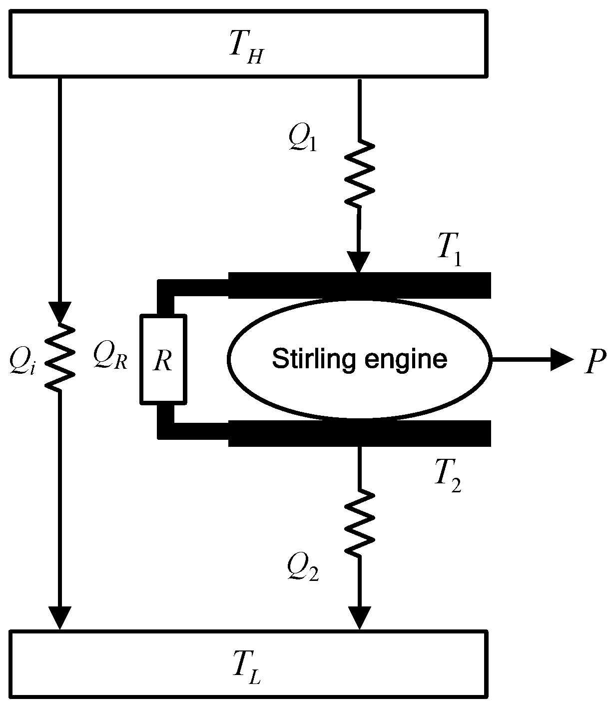
2. Model of SHE Cycle and OOs
3. Multi-Objective Optimizations
4. Conclusions
- From the expressions derived of the four OOs under linear phenomenological HTL it was found that , , and were obviously different from those in reference [69], which indicates that the change of HTL also fundamentally changes the performance indicators of the heat engine;
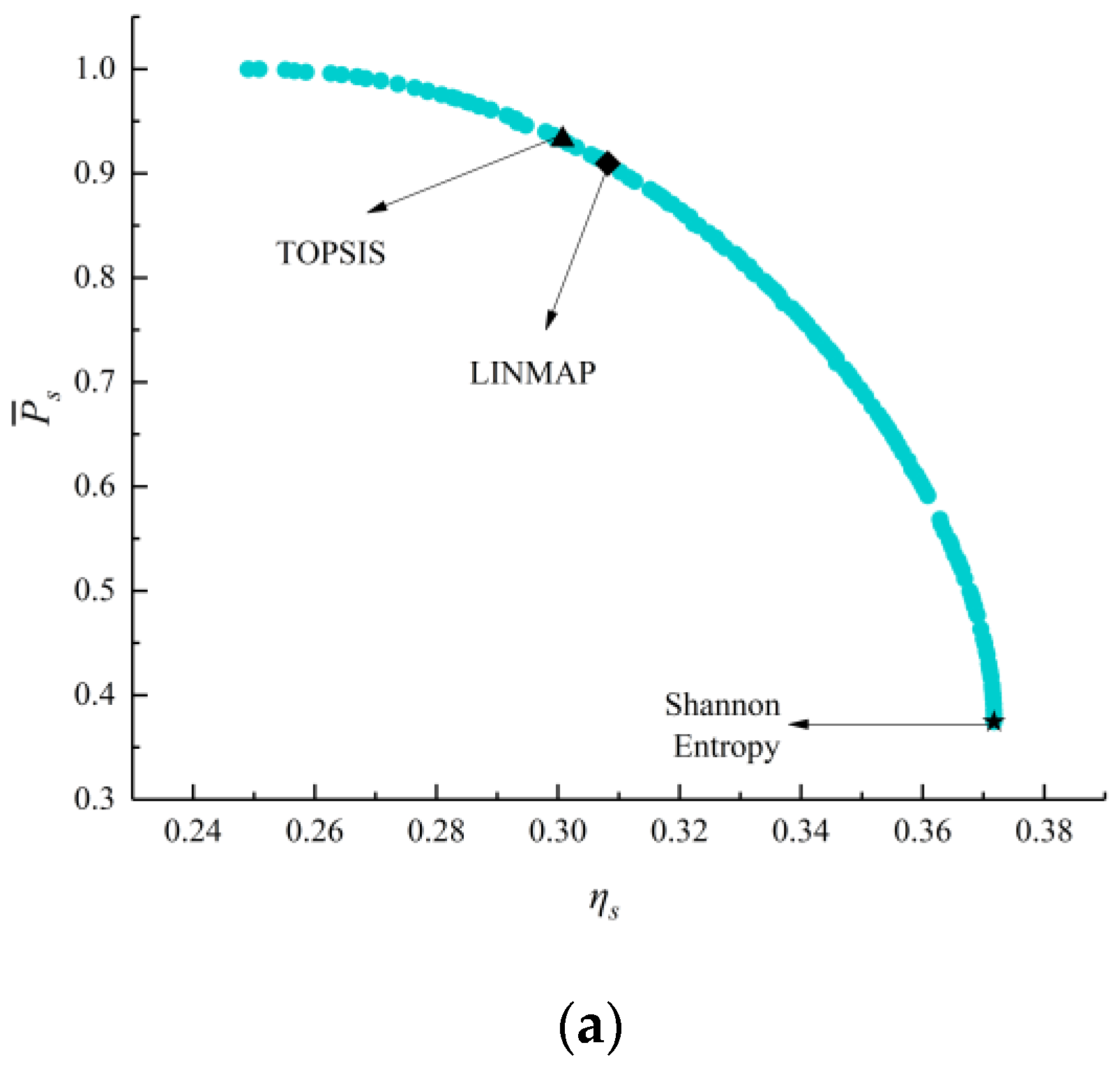
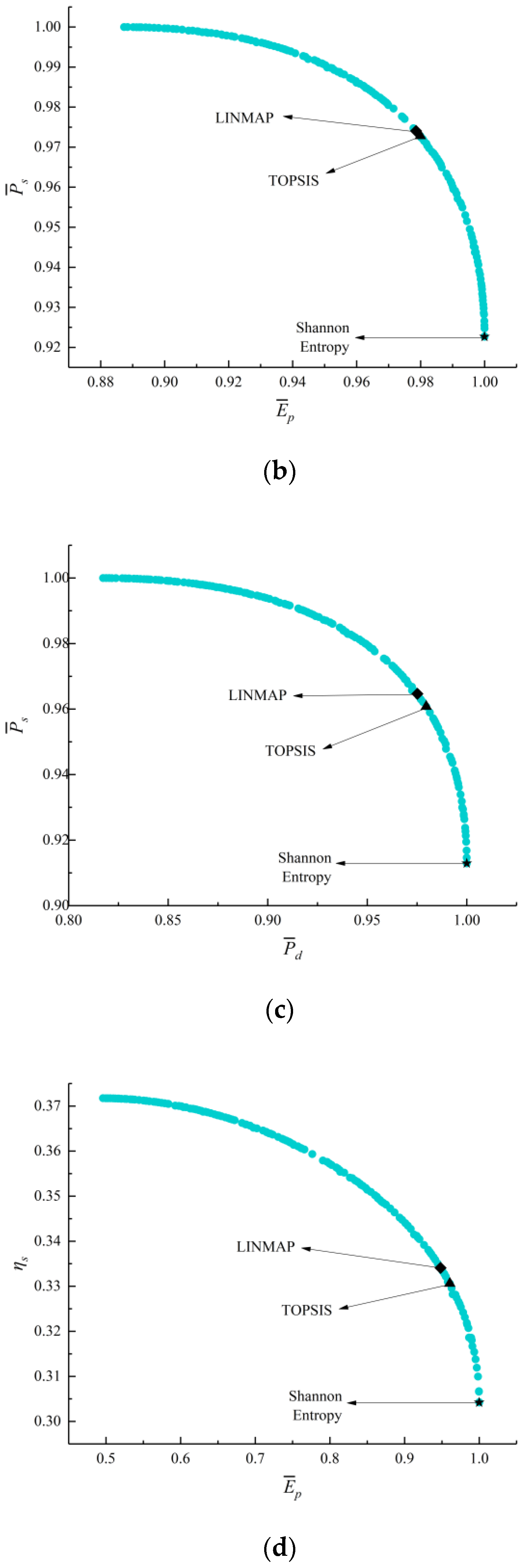
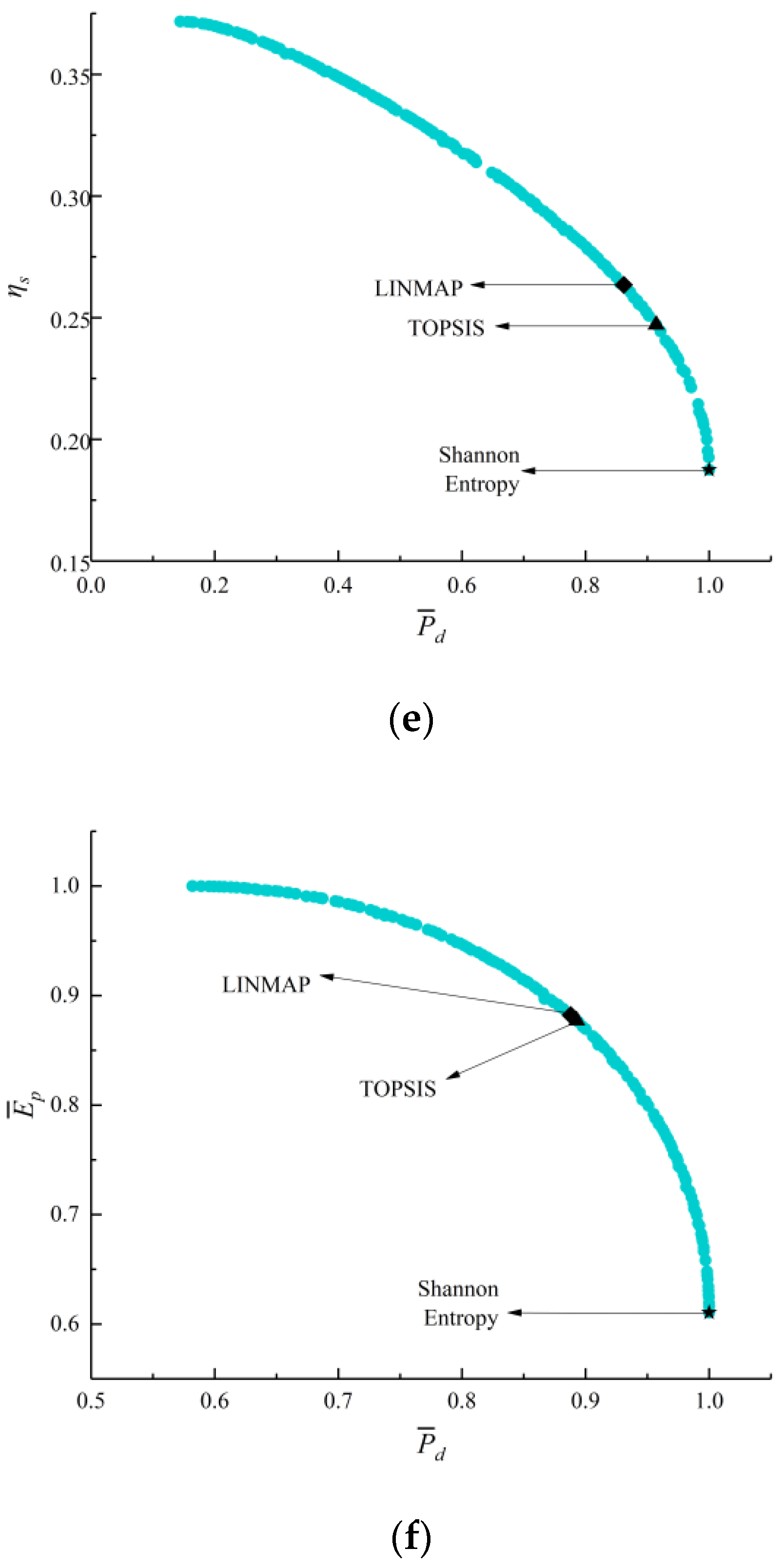
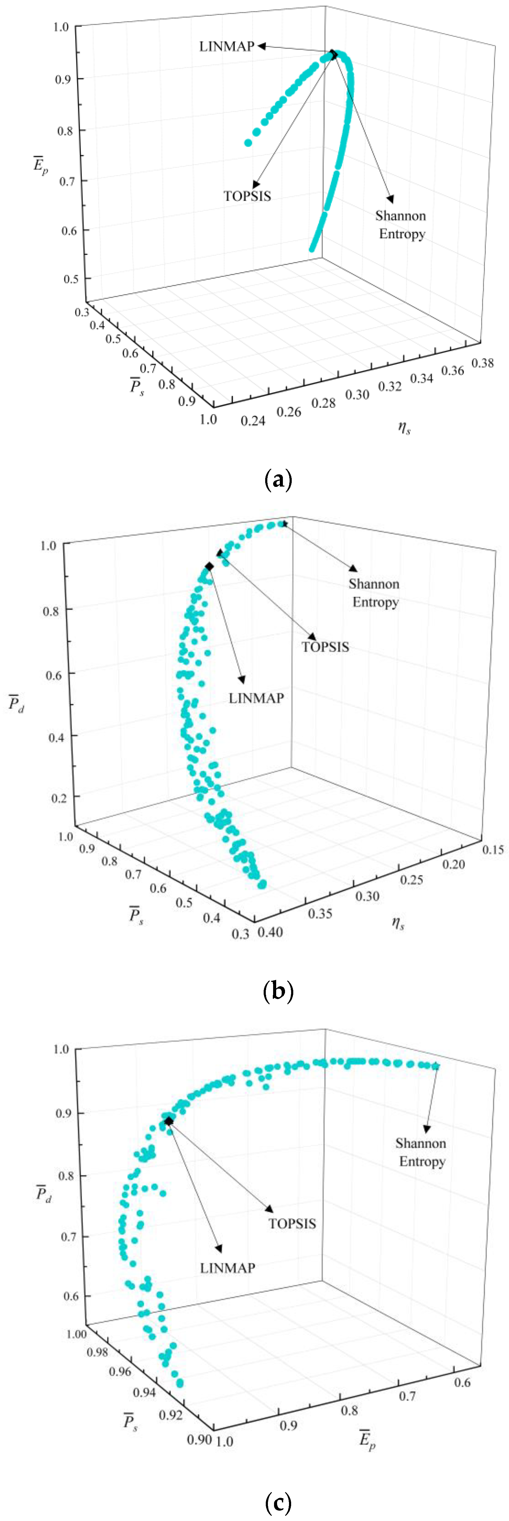
- The deviation indexes calculated by TOPSIS and LINMAP decision-making strategies are both 0.1683 when MOO is performed on , which are smaller and the optimization results are better than the results using the Shannon Entropy strategy. Compared with the deviation indexes (0.1978, 0.8624, 0.3319, and 0.3032) calculated by single-objective optimization at maximum , , , and conditions, the deviation indexes of MOO are smaller and their results are better;
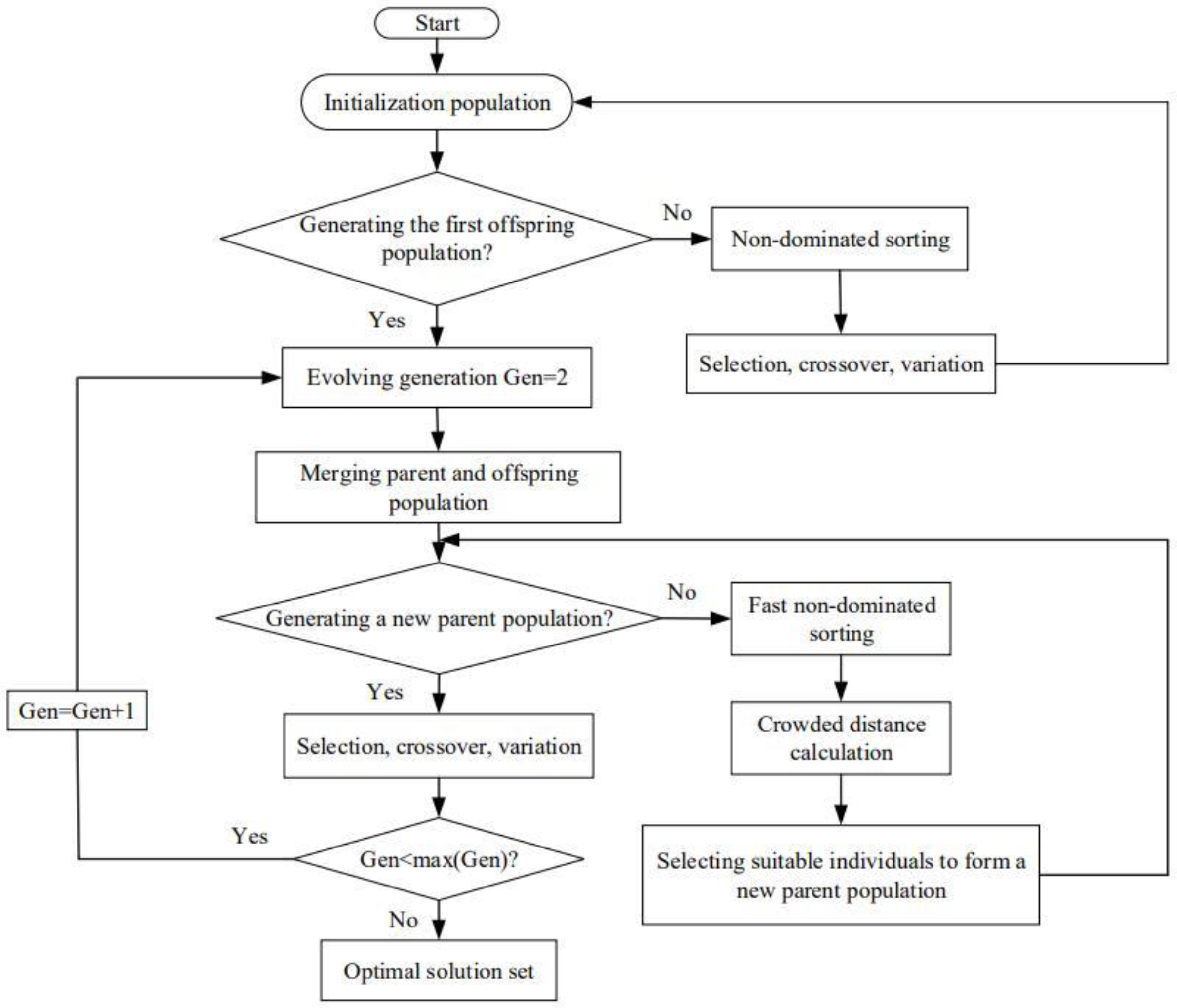
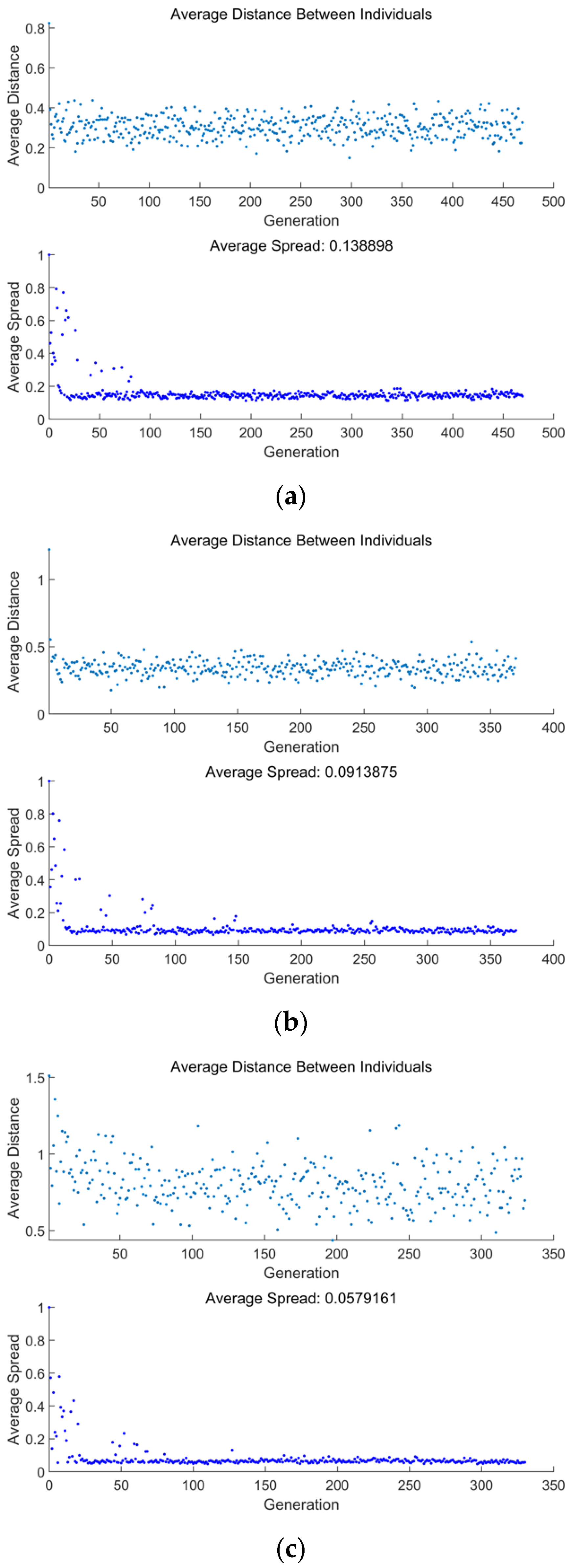
- When the genetic algorithm approaches convergence, which happens at the 331st generation for optimization, the genetic algorithm ends immediately. The average distance and spread gradually decrease from the beginning to the 25th generation, after which they remain stable until the end of the calculation. The average distance is mainly between 0.5~1.5, and the average spread keeps to nearly zero after the 25th generation, which suggests that the optimization process is nearly stable;
- When performing triple-objective optimizations, the MOO results of are better than the other combinations. The average distance mainly ranges from 0 to 0.5, and the average spread keeps to nearly zero after the 15th generation. When performing double-objective optimizations, the MOO results of are better than the other combinations. The average distance mainly ranges from 0.2 to 0.4, and the average spread keeps to nearly zero after the 20th generation;
- Compared with single-objective optimization, MOO can better take different OOs into account by choosing appropriate decision-making strategies. For the results of different objective combinations, appropriate schemes can be selected according to the actual design and operation to meet the requirements under different working conditions;
- FTT and MOO are effective tools to guide performance improvement and optimization for SHE cycles. The consideration of different HTLs is also necessary.
Author Contributions
Funding
Institutional Review Board Statement
Informed Consent Statement
Data Availability Statement
Acknowledgments
Conflicts of Interest
Nomenclature
| Buffer space | |
| Heat-leakage coefficient, | |
| Molar constant volume specific heat capacity, | |
| Mechanism effectiveness | |
| Flywheel | |
| Mechanical device | |
| Mole number, | |
| Regenerator | |
| Universal gas constant, | |
| Temperature, | |
| Time duration of the process, | |
| Volume, | |
| Compression work, J | |
| Expansion work, J | |
| Positive piston work, J | |
| Negative piston work, J | |
| Greek symbol | |
| , | Heat-transfer coefficient, |
| Volume–compression ratio | |
| Efficiency of the regenerator | |
| Cycle period, | |
| Entropy-generation rate, | |
| Subscripts | |
| Optimal | |
| Superscripts | |
| Dimensionless | |
| EP | Efficient power |
| FTT | Finite time thermodynamics |
| HT | Heat transfer |
| HTL | Heat-transfer law |
| MOO | Multi-objective optimization |
| OO | Optimization objective |
| PD | Power density |
| SHE | Stirling heat engine |
| WF | Working fluid |
References
- Curzon, F.L.; Ahlborn, B. Efficiency of a Carnot engine at maximum power output. Am. J. Phys. 1975, 43, 22–24. [Google Scholar] [CrossRef]
- Andresen, B. Finite-Time Thermodynamics; University of Copenhagen: København, Denmark, 1983. [Google Scholar]
- Hoffmann, K.H.; Burzler, J.M.; Schubert, S. Endoreversible thermodynamics. J. Non Equilib. Thermodyn. 1997, 22, 311–355. [Google Scholar]
- Chen, L.G.; Wu, C.; Sun, F.R. Finite time thermodynamic optimization or entropy generation minimization of energy systems. J. Non Equilib. Thermodyn. 1999, 24, 327–359. [Google Scholar] [CrossRef]
- Zhang, Y.; Lin, B.H.; Chen, J.C. Performance characteristics of an irreversible thermally driven Brownian microscopic heat engine. Eur. Phys. J. B 2006, 53, 481–485. [Google Scholar] [CrossRef]
- Açıkkalp, E.; Aras, H.; Hepbasli, A. Advanced exergoenvironmental assessment of a natural gas-fired electricity generating facility. Energy Convers. Manag. 2014, 81, 112–119. [Google Scholar] [CrossRef]
- Açıkkalp, E. Methods used for evaluation actual power generating thermal cycles and comparing them. Int. J. Electr. Power Energy Syst. 2015, 69, 85–89. [Google Scholar] [CrossRef]
- Ahmadi, M.H.; Ahmadi, M.A.; Pourfayaz, F. Thermal models for analysis of performance of Stirling engine: A review. Renew. Sustain. Energy Rev. 2017, 68, 168–184. [Google Scholar] [CrossRef]
- Yasunaga, T.; Ikegami, Y. Application of finite time thermodynamics for evaluation method of heat engines. Energy Proc. 2017, 129, 995–1001. [Google Scholar] [CrossRef]
- Kaushik, S.C.; Tyagi, S.K.; Kumar, P. Finite Time Thermodynamics of Power and Refrigeration Cycles; Springer: New York, NY, USA, 2018. [Google Scholar]
- Fontaine, K.; Yasunaga, T.; Ikegami, Y. OTEC maximum net power output using Carnot cycle and application to simplify heat exchanger selection. Entropy 2019, 21, 1143. [Google Scholar] [CrossRef]
- Feidt, M.; Costea, M. Progress in Carnot and Chambadal modeling of thermomechnical engine by considering entropy and heat transfer entropy. Entropy 2019, 21, 1232. [Google Scholar] [CrossRef]
- Patel, V.K.; Savsani, V.J.; Tawhid, M.A. Thermal System Optimization; Springer: Cham, Switzerland, 2019. [Google Scholar]
- Gonca, G.; Genc, I. Performance simulation of a double-reheat Rankine cycle mercury turbine system based on exergy. Int. J. Exergy 2019, 30, 392–403. [Google Scholar] [CrossRef]
- Gonca, G.; Sahin, B. Performance analysis of a novel eco-friendly internal combustion engine cycle. Int. J. Energy Res. 2019, 43, 5897–5911. [Google Scholar] [CrossRef]
- Gonca, G.; Hocaoglu, M.F. Performance Analysis and Simulation of a Diesel-Miller Cycle (DiMC) Engine. Arab. J. Sci. Eng. 2019, 44, 5811–5824. [Google Scholar] [CrossRef]
- Gonca, G.; Genc, I. Thermoecology-based performance simulation of a Gas-Mercury-Steam power generation system (GMSPGS). Energy Convers. Manag. 2019, 189, 91–104. [Google Scholar] [CrossRef]
- Feidt, M. Carnot cycle and heat engine: Fundamentals and applications. Entropy 2020, 22, 348. [Google Scholar] [CrossRef] [PubMed]
- Masser, R.; Hoffmann, K.H. Endoreversible modeling of a hydraulic recuperation system. Entropy 2020, 22, 383. [Google Scholar] [CrossRef]
- Kushner, A.; Lychagin, V.; Roop, M. Optimal thermodynamic processes for gases. Entropy 2020, 22, 448. [Google Scholar] [CrossRef]
- Berry, R.S.; Salamon, P.; Andresen, B. How it all began. Entropy 2020, 22, 908. [Google Scholar] [CrossRef]
- Feidt, M.; Costea, M. Effect of machine entropy production on the optimal performance of a refrigerator. Entropy 2020, 22, 913. [Google Scholar] [CrossRef]
- Ding, Z.M.; Ge, Y.L.; Chen, L.G.; Feng, H.J.; Xia, S.J. Optimal performance regions of Feynman’s ratchet engine with different optimization criteria. J. Non Equilib. Thermodyn. 2020, 45, 191–207. [Google Scholar] [CrossRef]
- Paul, R.; Hoffmann, K.H. A class of reduced-order regenerator models. Energies 2021, 14, 7295. [Google Scholar] [CrossRef]
- Gonca, G.; Hocaoglu, M.F. Exergy-based performance analysis and evaluation of a dual-diesel cycle engine. Therm. Sci. 2021, 25, 3675–3685. [Google Scholar] [CrossRef]
- Qi, C.Z.; Ding, Z.M.; Chen, L.G.; Ge, Y.L.; Feng, H.J. Modelling of irreversible two-stage combined thermal Brownian refrigerators and their optimal performance. J. Non Equilib. Thermodyn. 2021, 46, 175–189. [Google Scholar] [CrossRef]
- Andresen, B.; Salamon, P. Future perspectives of finite-time thermodynamics. Entropy 2022, 24, 690. [Google Scholar] [CrossRef]
- Gonca, G.; Sahin, B.; Genc, I. Investigation of maximum performance characteristics of seven-process cycle engine. Int. J. Exergy 2022, 37, 302–312. [Google Scholar] [CrossRef]
- Gonca, G.; Sahin, B. Performance investigation and evaluation of an engine operating on a modified dual cycle. Int. J. Energy Res. 2022, 46, 2454–2466. [Google Scholar] [CrossRef]
- Paul, R.; Hoffmann, K.H. Optimizing the piston paths of Stirling cycle cryocoolers. J. Non Equilib. Thermodyn. 2022, 47, 195–203. [Google Scholar] [CrossRef]
- Blank, D.A.; Davis, G.W.; Wu, C. Power optimization of an endoreversible Stirling cycle with regeneration. Energy 1994, 19, 125–133. [Google Scholar] [CrossRef]
- Chen, J.C. The effect of regenerative losses on the efficiency of a Stirling heat engine at maximum power output. Int. J. Ambient Energy 1997, 18, 107–112. [Google Scholar] [CrossRef]
- Chen, J.C.; Yan, Z.J.; Chen, L.X.; Andresen, B. Efficiency bound of a solar-driven Stirling heat engine system. Int. J. Energy Res. 1998, 22, 805–812. [Google Scholar] [CrossRef]
- Wu, F.; Chen, L.G.; Wu, C. Sun, F.R. Optimum performance of irreversible Stirling engine with imperfect regeneration. Energy Convers. Manag. 1998, 39, 727–732. [Google Scholar] [CrossRef]
- Tlili, I.; Timoumi, Y.; Nasrallah, S.B. Thermodynamic analysis of the Stirling heat engine with regenerative losses and internal irreversibilities. Int. J. Engine Res. 2008, 9, 45–56. [Google Scholar] [CrossRef]
- Tlili, I. Finite time thermodynamic evaluation of endoreversible Stirling heat engine at maximum power conditions. Renew. Sustain. Energy Rev. 2012, 16, 2234–2241. [Google Scholar] [CrossRef]
- Li, Y.Q.; He, Y.L.; Wang, W.W. Optimization of solar-powered Stirling heat engine with finite-time thermodynamics. Renew. Energy 2011, 36, 421–427. [Google Scholar]
- Ahmadi, M.H.; Ahmadi, M.A.; Mehrpooya, M. Investigation of the effect of design parameters on power output and thermal efficiency of a Stirling engine by thermodynamic analysis. Int. J. Low Carb. Technol. 2016, 11, 141–156. [Google Scholar] [CrossRef]
- Ahmed, F.; Huang, H.L.; Khan, A.M. Numerical modeling and optimization of beta-type Stirling engine. Appl. Therm. Eng. 2019, 149, 385–400. [Google Scholar] [CrossRef]
- Ramachandran, S.; Kumar, N.; Timmaraju, M.V. Thermodynamic analysis of solar low-temperature differential Stirling engine considering imperfect regeneration and thermal losses. J. Sol. Energy Eng. 2020, 142, 051012. [Google Scholar] [CrossRef]
- Ahadi, F.; Azadi, M.; Biglari, M.; Madani, S.N. Study of coating effects on the performance of Stirling engine by non-ideal adiabatic thermodynamics modeling. Energy Rep. 2021, 7, 3688–3702. [Google Scholar] [CrossRef]
- de Moura, E.F.; Henriques, I.B.; Ribeiro, G.B. Thermodynamic-dynamic coupling of a Stirling engine for space exploration. Therm. Sci. Eng. Prog. 2022, 32, 101320. [Google Scholar] [CrossRef]
- Purkait, C.; Biswas, A. Performance of Heisenberg-coupled spins as quantum Stirling heat machine near quantum critical point. Phys. Lett. A 2022, 442, 128180. [Google Scholar] [CrossRef]
- Kitaya, K.; Isobe, M. Molecular dynamics study of a nano-scale β-type Stirling engine. J. Phys. Conf. Ser. 2022, 2207, 012006. [Google Scholar] [CrossRef]
- Sahin, B.; Kodal, A.; Yavuz, H. Efficiency of a Joule-Brayton engine at maximum power density. J. Phys. D Appl. Phys. 1995, 28, 1309. [Google Scholar] [CrossRef]
- Chen, L.G.; Zheng, J.L.; Sun, F.R.; Wu, C. Performance comparison of an endoreversible closed variable temperature heat reservoir Brayton cycle under maximum power density and maximum power conditions. Energy Convers. Manag. 2002, 43, 33–43. [Google Scholar] [CrossRef]
- Ust, Y. A comparative performance analysis and optimization of irreversible Atkinson cycle under maximum power density and maximum power conditions. Int. J. Thermophys. 2009, 30, 1001–1013. [Google Scholar] [CrossRef]
- Gonca, G. Performance analysis and optimization of irreversible Dual-Atkinson Cycle Engine (DACE) with heat transfer effects under maximum power and maximum power density conditions. Appl. Math. Model. 2016, 40, 6725–6736. [Google Scholar] [CrossRef]
- Karakurt, A.S.; Bashan, V.; Ust, Y. Comparative maximum power density analysis of a supercritical CO2 Brayton power cycle. J. Therm. Eng. 2020, 6, 50–57. [Google Scholar] [CrossRef]
- Yan, Z.J. η and P of a Carnot engine at maximum ηP. Chin. J. Nat. 1984, 7, 475. (In Chinese) [Google Scholar]
- Yilmaz, T. A new performance criterion for heat engines: Efficient power. J. Energy Inst. 2006, 79, 38–41. [Google Scholar] [CrossRef]
- Kumar, R.; Kaushik, S.C.; Kumar, R. Efficient power of Brayton heat engine with friction. Int. J. Eng. Res. Technol. 2013, 6, 643–650. [Google Scholar]
- Patodi, K.; Maheshwari, G. Performance analysis of an Atkinson cycle with variable specific-heats of the working fluid under maximum efficient power conditions. Int. J. Low Carbon Technol. 2013, 8, 289–294. [Google Scholar] [CrossRef]
- Nilavarasi, K.; Ponmurugan, M. Optimized efficiency at maximum figure of merit and efficient power of power law dissipative Carnot like heat engines. J. Stat. Mech. Theory Exp. 2021, 2021, 043208. [Google Scholar] [CrossRef]
- Tian, L.; Chen, L.G.; Ren, T.T.; Ge, Y.L.; Feng, H.J. Optimal distribution of heat exchanger area for maximum efficient power of thermoelectric generators. Energy Rep. 2022, 8, 10492–10500. [Google Scholar] [CrossRef]
- Ahmadi, M.H.; Hosseinzade, H.; Sayyaadi, H.; Mohammadi, A.H.; Kimiaghalam, F. Application of the multi-objective optimization method for designing a powered Stirling heat engine: Design with maximized power, thermal efficiency and minimized pressure loss. Renew. Energy 2013, 60, 313–322. [Google Scholar] [CrossRef]
- Ahmadi, M.H.; Mohammadi, A.H.; Dehghani, S.; Barranco-Jiménez, M.A. Multi-objective thermodynamic-based optimization of output power of Solar Dish-Stirling engine by implementing an evolutionary algorithm. Energy Convers. Manag. 2013, 75, 438–445. [Google Scholar] [CrossRef]
- Ahmadi, M.H.; Ahmadi, M.A.; Pourfayaz, F.; Hosseinzade, H.; Acıkkalp, E.; Tlili, I.; Feidt, M. Designing a powered combined Otto and Stirling cycle power plant through multi-objective optimization approach. Renew. Sustain. Energy Rev. 2016, 62, 585–595. [Google Scholar] [CrossRef]
- Luo, Z.Y.; Sultan, U.; Ni, M.J.; Peng, H.; Shi, B.W.; Xiao, G. Multi-objective optimization for GPU3 Stirling engine by combining multi-objective algorithms. Renew. Energy 2016, 94, 114–125. [Google Scholar] [CrossRef]
- Punnathanam, V.; Kotecha, P. Effective multi-objective optimization of Stirling engine systems. Appl. Therm. Eng. 2016, 108, 261–276. [Google Scholar] [CrossRef]
- Hooshang, M.; Toghyani, S.; Kasaeian, A.; Moghadam, R.A.; Ahmadi, M.H. Enhancing and multi-objective optimising of the performance of Stirling engine using third-order thermodynamic analysis. Int. J. Ambient Energy 2018, 39, 382–391. [Google Scholar] [CrossRef]
- Dai, D.D.; Yuan, F.; Long, R.; Liu, Z.C.; Liu, W. Performance analysis and multi-objective optimization of a Stirling engine based on MOPSOCD. Int. J. Therm. Sci. 2018, 124, 399–406. [Google Scholar] [CrossRef]
- Ye, W.L.; Yang, P.; Liu, Y.W. Multi-objective thermodynamic optimization of a free piston Stirling engine using response surface methodology. Energy Convers. Manag. 2018, 176, 147–163. [Google Scholar] [CrossRef]
- Shah, P.; Saliya, P.; Raja, B.; Patel, V. A multiobjective thermodynamic optimization of a nanoscale Stirling engine operated with Maxwell-Boltzmann gas. Heat Transfer—Asian Res. 2019, 48, 1913–1932. [Google Scholar] [CrossRef]
- Shakouri, O.; Ahmadi, M.H.; Gord, M.F. Thermodynamic assessment and performance optimization of solid oxide fuel cell-Stirling heat engine-reverse osmosis desalination. Int. J. Low Carbon Technol. 2021, 16, 417–428. [Google Scholar] [CrossRef]
- Ahmed, F.; Zhu, S.M.; Yu, G.Y.; Luo, E.C. A potent numerical model coupled with multi-objective NSGA-II algorithm for the optimal design of Stirling engine. Energy 2022, 247, 123468. [Google Scholar] [CrossRef]
- Senft, J.R. Theoretical limits on the performance of Stirling engines. Int. J. Energy Res. 1998, 22, 991–1000. [Google Scholar] [CrossRef]
- Senft, J.R. Mechanical Efficiency of Heat Engines; Cambridge University Press: Cambridge, UK, 2007. [Google Scholar]
- Xu, H.R.; Chen, L.G.; Ge, Y.L.; Feng, H.J. Multi-objective optimization of Stirling heat engine with various heat transfer and mechanical losses. Energy 2022, 256, 124699. [Google Scholar] [CrossRef]
- Wu, C. Power optimization of a finite-time solar radiant heat engine. Int. J. Ambient Energy 1989, 10, 145–150. [Google Scholar] [CrossRef]
- Wu, C. Optimal power from a radiating solar-powered thermionic engine. Energy Convers. Manag. 1992, 33, 279–282. [Google Scholar] [CrossRef]
- Goktun, S.; Ozkaynak, S.; Yavuz, H. Design parameters of a radiative heat engine. Energy 1993, 18, 651–655. [Google Scholar] [CrossRef]
- Angulo-Brown, F.; Paez-Hernandez, R. Endoreversible thermal cycle with a nonlinear heat transfer law. J. Appl. Phys. 1993, 74, 2216–2219. [Google Scholar] [CrossRef]
- Huleihil, M.; Andresen, B. Convective heat transfer law for an endoreversible engine. J. Appl. Phys. 2006, 100, 014911. [Google Scholar] [CrossRef]
- Chen, L.G.; Li, J.; Sun, F.R. Generalized irreversible heat-engine experiencing a complex heat-transfer law. Appl. Energy 2008, 85, 52–60. [Google Scholar] [CrossRef]
- Li, J.; Chen, L.G. Optimal configuration of finite source heat engine cycle for maximum output work with complex heat transfer law. J. Non Equilib. Thermodyn. 2022, 47, 433–441. [Google Scholar] [CrossRef]
- Chen, L.G.; Xia, S.J. Heat engine cycle configurations for maximum work output with generalized models of reservoir thermal capacity and heat resistance. J. Non Equilib. Thermodyn. 2022, 47, 329–338. [Google Scholar] [CrossRef]
- Ding, Z.M.; Chen, L.G.; Sun, F.R. Performance optimization of a linear phenomenological law system Stirling engine. J. Energy Inst. 2015, 88, 36–42. [Google Scholar] [CrossRef]
- Deb, K.; Pratap, A.; Agarwal, S.; Meyarivan, T. A fast and elitist multiobjective genetic algorithm: NSGA-II. IEEE Trans. Evol. Comput. 2002, 6, 182–197. [Google Scholar] [CrossRef]
- Yusuf, A.; Bayhan, N.; Tiryaki, H.; Hamawandi, B.; Toprak, M.S.; Ballikaya, S. Multi-objective optimization of concentrated photovoltaic-thermoelectric hybrid system via non-dominated sorting genetic algorithm (NSGA II). Energy Convers. Manag. 2021, 236, 114065. [Google Scholar] [CrossRef]
- Xiao, W.; Cheng, A.D.; Li, S.; Jiang, X.B.; Ruan, X.H.; He, G.H. A multi-objective optimization strategy of steam power system to achieve standard emission and optimal economic by NSGA-Ⅱ. Energy 2021, 232, 120953. [Google Scholar] [CrossRef]
- Soleimani, S.; Eckels, S. Multi-objective optimization of 3D micro-fins using NSGA-II. Int. J. Heat Mass Transfer 2022, 197, 123315. [Google Scholar] [CrossRef]
- Arora, R.; Kaushik, S.C.; Kumar, R.; Arora, R. Soft computing based multi-objective optimization of Brayton cycle power plant with isothermal heat addition using evolutionary algorithm and decision making. Appl. Soft Comput. 2016, 46, 267–283. [Google Scholar] [CrossRef]
- Hwang, C.L.; Yoon, K. Multiple Attribute Decision Making-Methods and Applications a State of the Art Survey; Springer: New York, NY, USA, 1981. [Google Scholar]
- Etghani, M.M.; Shojaeefard, M.H.; Khalkhali, A.; Akbari, M. A hybrid method of modified NSGA-II and Topsis to optimize performance and emissions of a diesel engine using biodiesel. Appl. Therm. Eng. 2013, 59, 309–315. [Google Scholar] [CrossRef]
- Kamali, H.; Mehrpooya, M.; Mousavi, S.H.; Ganjali, M.R. Thermally regenerative electrochemical refrigerators decision-making process and multi-objective optimization. Energy Convers. Manag. 2022, 252, 115060. [Google Scholar] [CrossRef]
- Sayyaadi, H.; Mehrabipour, R. Efficiency enhancement of a gas turbine cycle using an optimized tubular recuperative heat exchanger. Energy 2012, 38, 362–375. [Google Scholar] [CrossRef]
- Khanmohammadi, S.; Musharavati, F. Multi-generation energy system based on geothermal source to produce power, cooling, heating, and fresh water: Exergoeconomic analysis and optimum selection by LINMAP method. Appl. Therm. Eng. 2021, 195, 117127. [Google Scholar] [CrossRef]
- Guisado, J.; Morales, F.J.; Guerra, J. Application of Shannon’s entropy to classify emergent behaviors in a simulation of laser dynamics. Math. Comput. Modell. 2005, 42, 847–854. [Google Scholar] [CrossRef]
- Zang, P.C.; Chen, L.G.; Ge, Y.L.; Shi, S.S.; Feng, H.J. Four-objective optimization for an irreversible Porous Medium cycle with linear variation in working fluid’s specific heat. Entropy 2022, 24, 1074. [Google Scholar] [CrossRef]


| Parameters | Values |
|---|---|
| Generations | 700 |
| Population size | 300 |
| Pareto fraction | 0.5 |
| Crossover fraction | 0.8 |
| Optimization Methods | Decision- Making Strategies | Optimization Variables | Optimization Objectives | Deviation Index | ||||
|---|---|---|---|---|---|---|---|---|
| Four-objective optimization ) | LINMAP | 0.5815 | 1.5301 | 0.9608 | 0.2601 | 0.8905 | 0.8721 | 0.1683 |
| TOPSIS | 0.5815 | 1.5301 | 0.9608 | 0.2601 | 0.8905 | 0.8721 | 0.1683 | |
| Shannon Entropy | 0.6610 | 1.2684 | 0.9128 | 0.1877 | 0.6103 | 1.0000 | 0.3018 | |
| Three-objective optimization ) | LINMAP | 0.5462 | 2.2788 | 0.9178 | 0.3056 | 0.9995 | 0.5597 | 0.3455 |
| TOPSIS | 0.5475 | 2.2032 | 0.9226 | 0.3042 | 1.0000 | 0.5819 | 0.3306 | |
| Shannon Entropy | 0.5475 | 2.2032 | 0.9226 | 0.3042 | 1.0000 | 0.5819 | 0.3306 | |
| Three-objective optimization ) | LINMAP | 0.5885 | 1.5360 | 0.9670 | 0.2576 | 0.8903 | 0.8775 | 0.1648 |
| TOPSIS | 0.5968 | 1.4652 | 0.9658 | 0.2462 | 0.8475 | 0.9161 | 0.1735 | |
| Shannon Entropy | 0.6611 | 1.2679 | 0.9124 | 0.1875 | 0.6095 | 1.0000 | 0.3022 | |
| Three-objective optimization ) | LINMAP | 0.6030 | 1.5375 | 0.9835 | 0.2512 | 0.8802 | 0.8889 | 0.1641 |
| TOPSIS | 0.6030 | 1.5375 | 0.9835 | 0.2512 | 0.8802 | 0.8889 | 0.1641 | |
| Shannon Entropy | 0.6610 | 1.2686 | 0.9129 | 0.1877 | 0.6106 | 1.0000 | 0.3016 | |
| Three-objective optimization ) | LINMAP | 0.5718 | 1.2686 | 0.9502 | 0.2663 | 0.9017 | 0.8509 | 0.1756 |
| TOPSIS | 0.5852 | 1.5303 | 0.9653 | 0.2584 | 0.8890 | 0.8766 | 0.1663 | |
| Shannon Entropy | 0.6610 | 1.2686 | 0.9129 | 0.1877 | 0.6106 | 1.0000 | 0.3016 | |
| Two-objective optimization ) | LINMAP | 0.5407 | 2.1898 | 0.9095 | 0.3082 | 0.9988 | 0.5771 | 0.3367 |
| TOPSIS | 0.5531 | 2.2047 | 0.9325 | 0.3008 | 0.9992 | 0.5877 | 0.3250 | |
| Shannon Entropy | 0.4208 | 3.6089 | 0.3745 | 0.3718 | 0.4962 | 0.1442 | 0.8630 | |
| Two-objective optimization ) | LINMAP | 0.5793 | 1.9746 | 0.9740 | 0.2820 | 0.9786 | 0.6855 | 0.2580 |
| TOPSIS | 0.5783 | 1.9812 | 0.9728 | 0.2827 | 0.9799 | 0.6824 | 0.2600 | |
| Shannon Entropy | 0.5476 | 2.2031 | 0.9227 | 0.3042 | 1.0000 | 0.5820 | 0.3305 | |
| Two-objective optimization ) | LINMAP | 0.6459 | 1.3747 | 0.9647 | 0.2141 | 0.7360 | 0.9752 | 0.2286 |
| TOPSIS | 0.6468 | 1.3629 | 0.9608 | 0.2120 | 0.7257 | 0.9796 | 0.2345 | |
| Shannon Entropy | 0.6610 | 1.2686 | 0.9129 | 0.1877 | 0.6107 | 1.0000 | 0.3016 | |
| Two-objective optimization ) | LINMAP | 0.5026 | 2.6195 | 0.7965 | 0.3341 | 0.9482 | 0.4226 | 0.4700 |
| TOPSIS | 0.5079 | 2.5508 | 0.8154 | 0.3306 | 0.9605 | 0.4442 | 0.4491 | |
| Shannon Entropy | 0.5475 | 2.2033 | 0.9226 | 0.3042 | 1.0000 | 0.5819 | 0.3306 | |
| Two-objective optimization ) | LINMAP | 0.5709 | 1.5216 | 0.9439 | 0.2835 | 0.8861 | 0.8620 | 0.1782 |
| TOPSIS | 0.5898 | 1.4515 | 0.9551 | 0.2471 | 0.8410 | 0.9144 | 0.1792 | |
| Shannon Entropy | 0.6614 | 1.2682 | 0.9126 | 0.1875 | 0.6098 | 1.0000 | 0.3021 | |
| Two-objective optimization ) | LINMAP | 0.5989 | 1.5332 | 0.9797 | 0.2527 | 0.8821 | 0.8879 | 0.1636 |
| TOPSIS | 0.5984 | 1.5217 | 0.9777 | 0.2518 | 0.8772 | 0.8928 | 0.1642 | |
| Shannon Entropy | 0.6610 | 1.2686 | 0.9129 | 0.1877 | 0.6106 | 1.0000 | 0.3016 | |
| - | 0.6229 | 1.7047 | 1.0000 | 0.2501 | 0.8909 | 0.8152 | 0.1978 | |
| - | 0.4213 | 3.6042 | 0.3777 | 0.3718 | 0.5003 | 0.1456 | 0.8624 | |
| - | 0.5469 | 2.2063 | 0.9213 | 0.3046 | 1.0000 | 0.5803 | 0.3319 | |
| - | 0.6626 | 1.2676 | 0.9121 | 0.1870 | 0.6078 | 1.0000 | 0.3032 | |
| Positive ideal point | - | - | 1.0000 | 0.3718 | 1.0000 | 1.0000 | - | |
| Negative ideal point | - | - | 0.3745 | 0.1854 | 0.4962 | 0.1442 | - | |
Publisher’s Note: MDPI stays neutral with regard to jurisdictional claims in published maps and institutional affiliations. |
© 2022 by the authors. Licensee MDPI, Basel, Switzerland. This article is an open access article distributed under the terms and conditions of the Creative Commons Attribution (CC BY) license (https://creativecommons.org/licenses/by/4.0/).
Share and Cite
Xu, H.; Chen, L.; Ge, Y.; Feng, H. Four-Objective Optimization of an Irreversible Stirling Heat Engine with Linear Phenomenological Heat-Transfer Law. Entropy 2022, 24, 1491. https://doi.org/10.3390/e24101491
Xu H, Chen L, Ge Y, Feng H. Four-Objective Optimization of an Irreversible Stirling Heat Engine with Linear Phenomenological Heat-Transfer Law. Entropy. 2022; 24(10):1491. https://doi.org/10.3390/e24101491
Chicago/Turabian StyleXu, Haoran, Lingen Chen, Yanlin Ge, and Huijun Feng. 2022. "Four-Objective Optimization of an Irreversible Stirling Heat Engine with Linear Phenomenological Heat-Transfer Law" Entropy 24, no. 10: 1491. https://doi.org/10.3390/e24101491
APA StyleXu, H., Chen, L., Ge, Y., & Feng, H. (2022). Four-Objective Optimization of an Irreversible Stirling Heat Engine with Linear Phenomenological Heat-Transfer Law. Entropy, 24(10), 1491. https://doi.org/10.3390/e24101491