Author Contributions
Conceptualization, L.G.-P., J.G.-C., R.A.-S. and J.C.L.; Formal analysis, L.G.-P., J.G.-C., R.A.-S. and J.C.L.; Methodology, L.G.-P., J.G.-C., R.A.-S. and J.C.L.; Project administration, L.G.-P., J.G.-C., R.A.-S. and J.C.L.; Software, L.G.-P., J.G.-C., R.A.-S. and J.C.L.; Supervision, L.G.-P., J.G.-C., R.A.-S. and J.C.L.; Validation, L.G.-P., J.G.-C., R.A.-S. and J.C.L.; Writing—original draft, L.G.-P., J.G.-C., R.A.-S. and J.C.L.; Writing—review & editing, L.G.-P., J.G.-C., R.A.-S. and J.C.L. All authors have read and agreed to the published version of the manuscript.
Figure 1.
Stability region for () in the absence of memory. The area with no economic sense is shaded in blue, that is, when .
Figure 1.
Stability region for () in the absence of memory. The area with no economic sense is shaded in blue, that is, when .
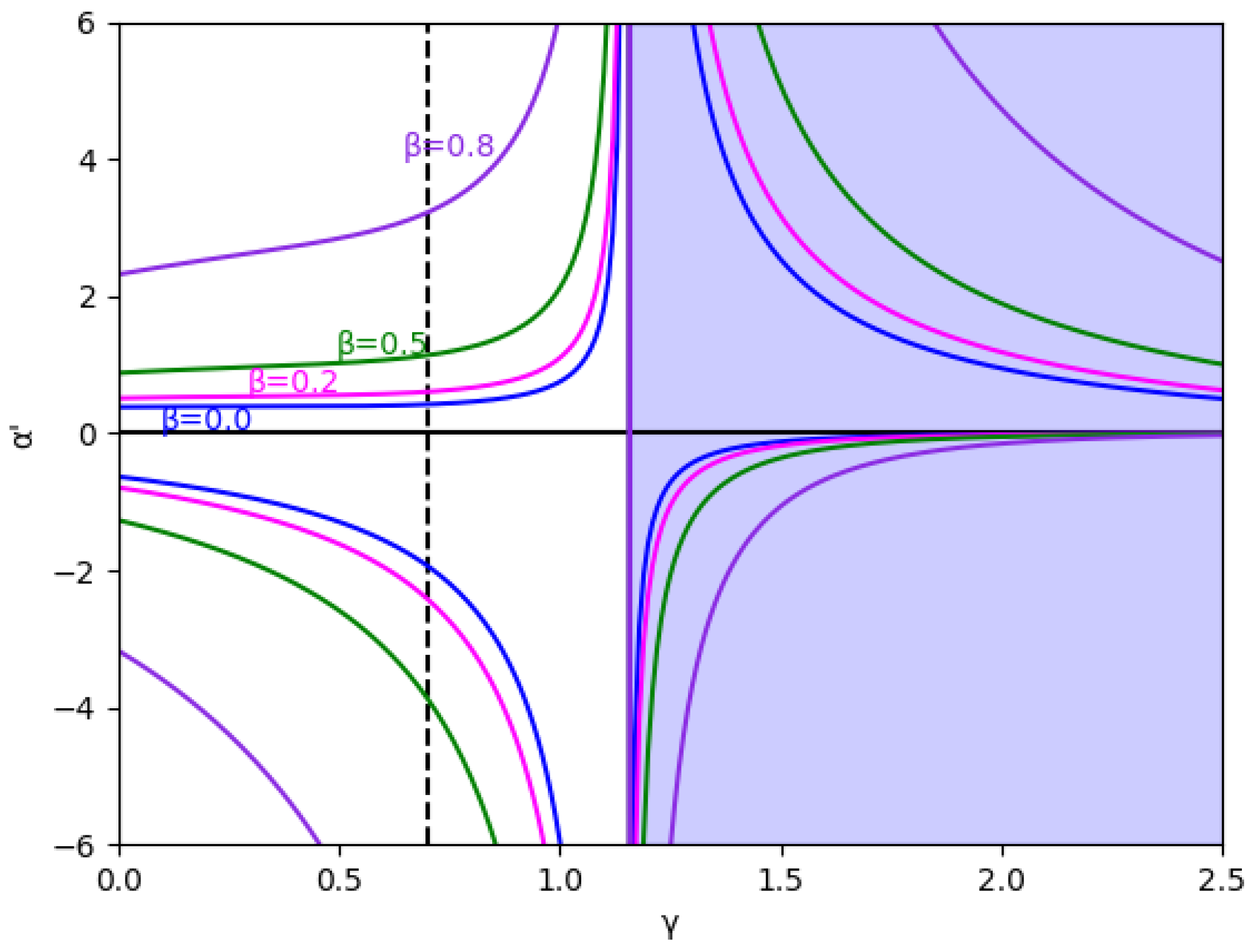
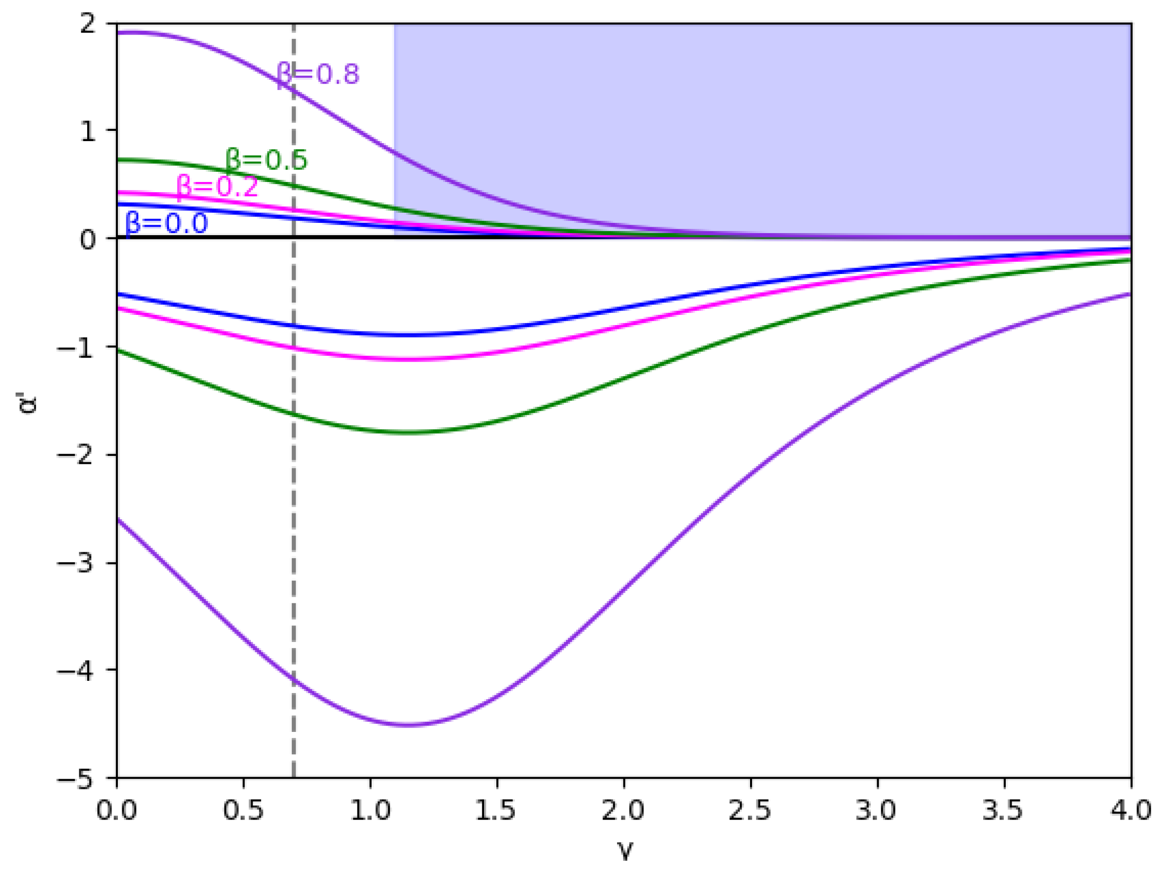
Figure 2.
Stability region for () and different values of (0, 0.2, 0.5, and 0.8). The vertical line is represented because this value and are the values used in the bifurcation diagrams. The area with no economic sense is shaded in blue, that is, when .
Figure 2.
Stability region for () and different values of (0, 0.2, 0.5, and 0.8). The vertical line is represented because this value and are the values used in the bifurcation diagrams. The area with no economic sense is shaded in blue, that is, when .
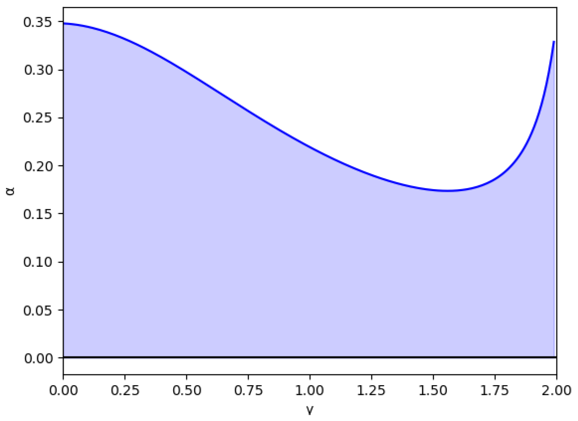
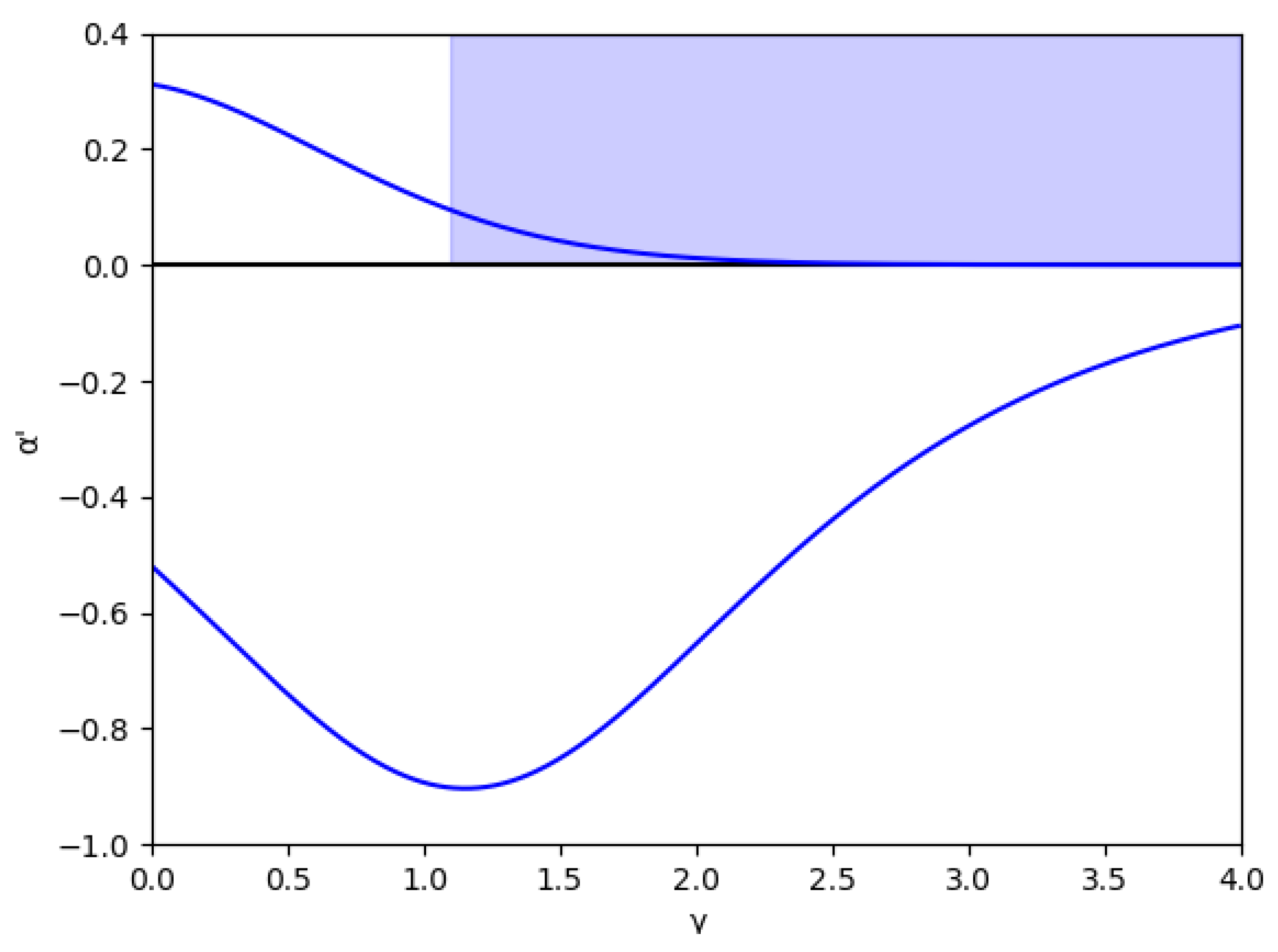
Figure 3.
Stability region as a function of for () and without memory, .
Figure 3.
Stability region as a function of for () and without memory, .
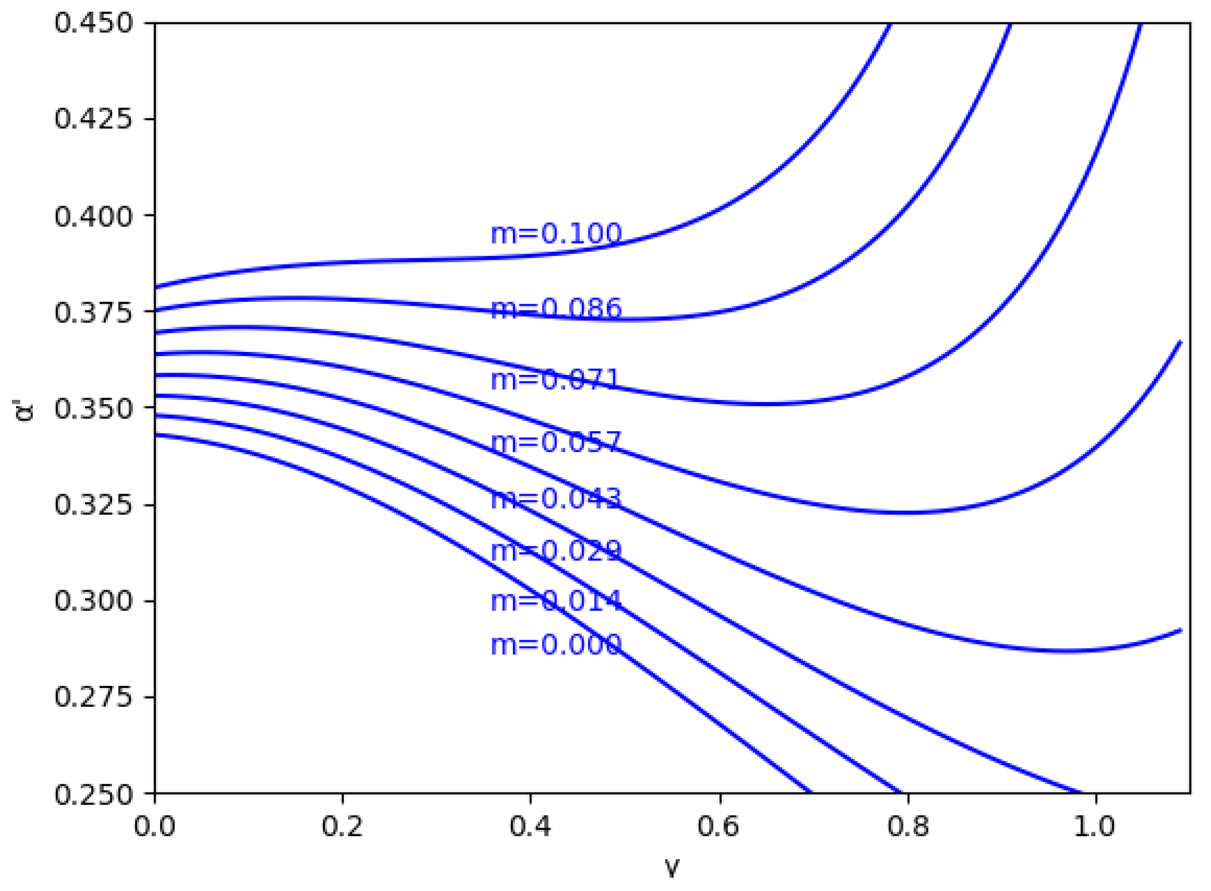
Figure 4.
Stability region as a function of for m between and without memory, .
Figure 4.
Stability region as a function of for m between and without memory, .
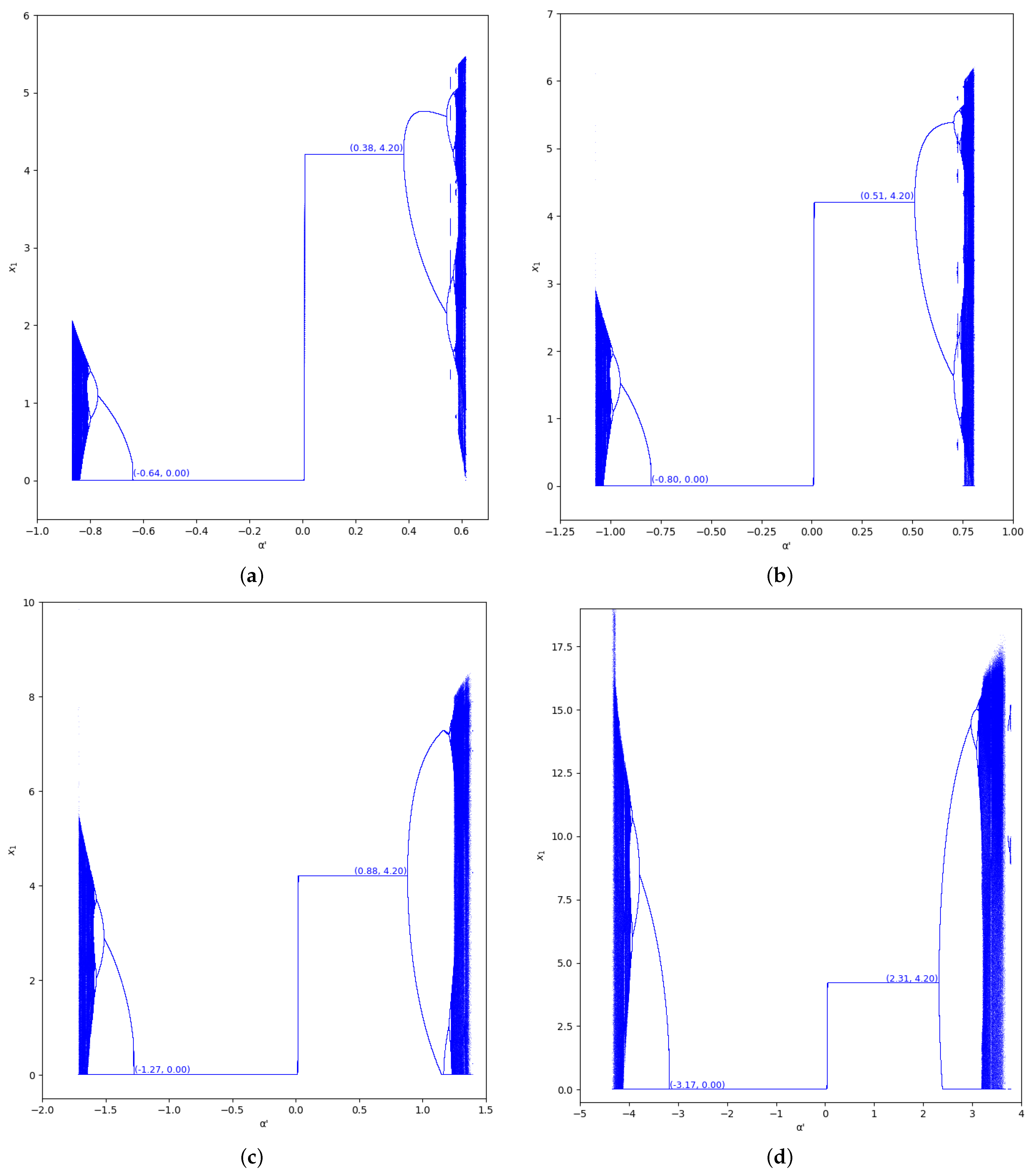
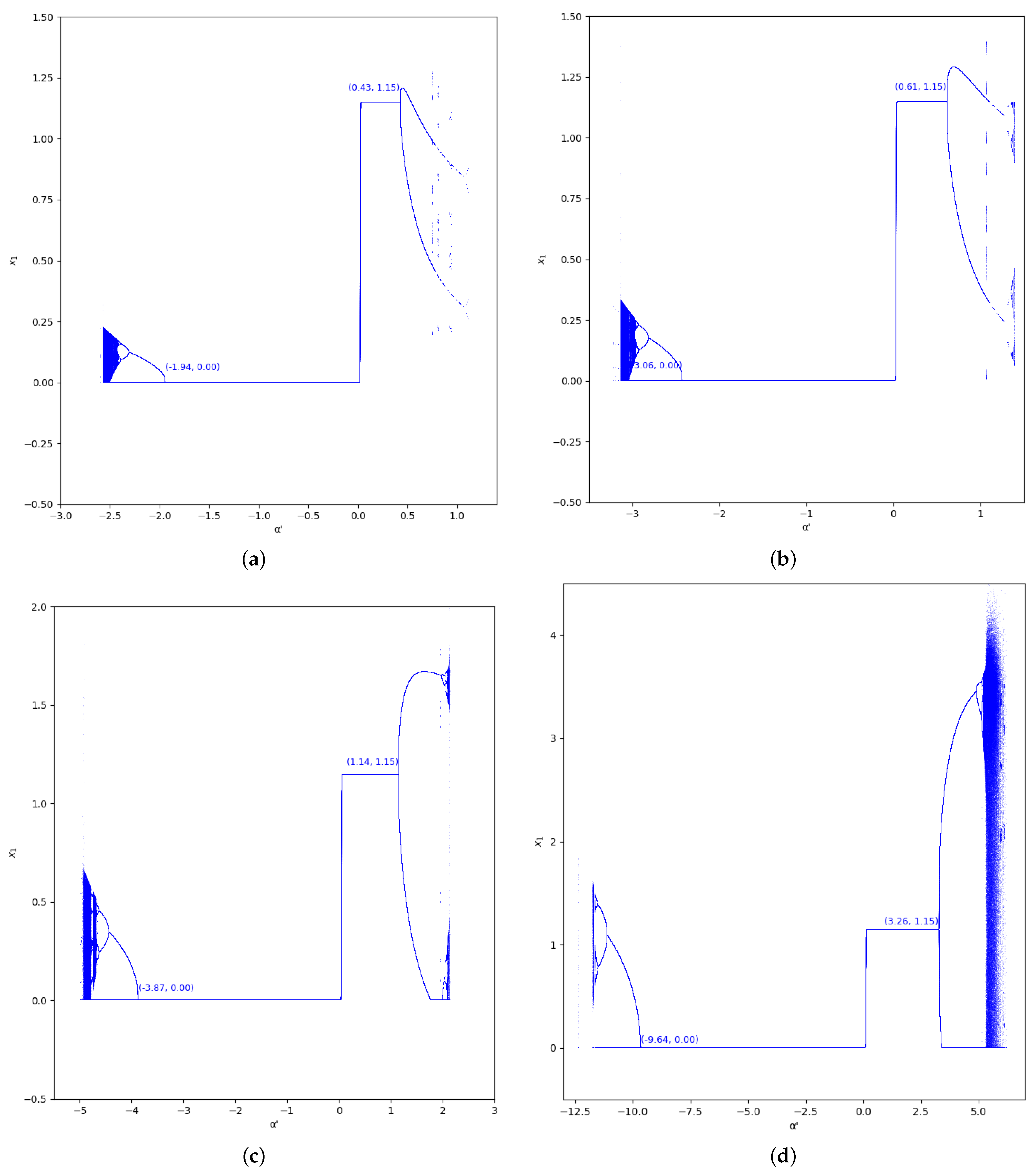
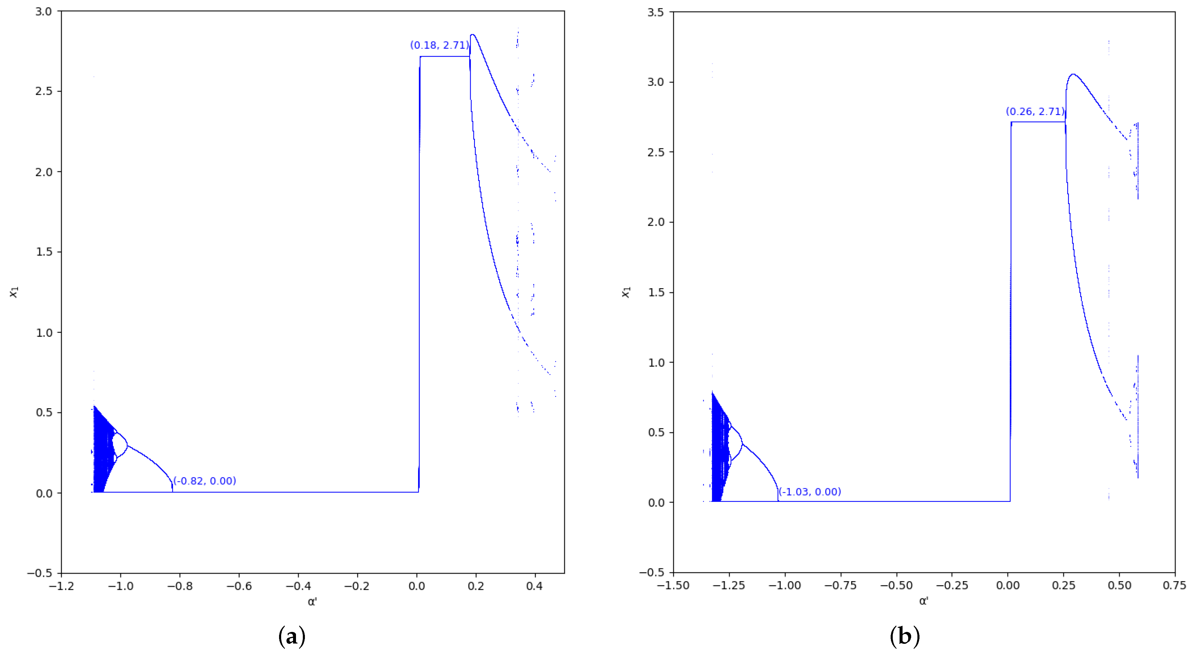
Figure 5.
Bifurcation diagrams of output of the first player as a function of with and in the zone (). (a) ; (b) ; (c) ; (d) .
Figure 5.
Bifurcation diagrams of output of the first player as a function of with and in the zone (). (a) ; (b) ; (c) ; (d) .
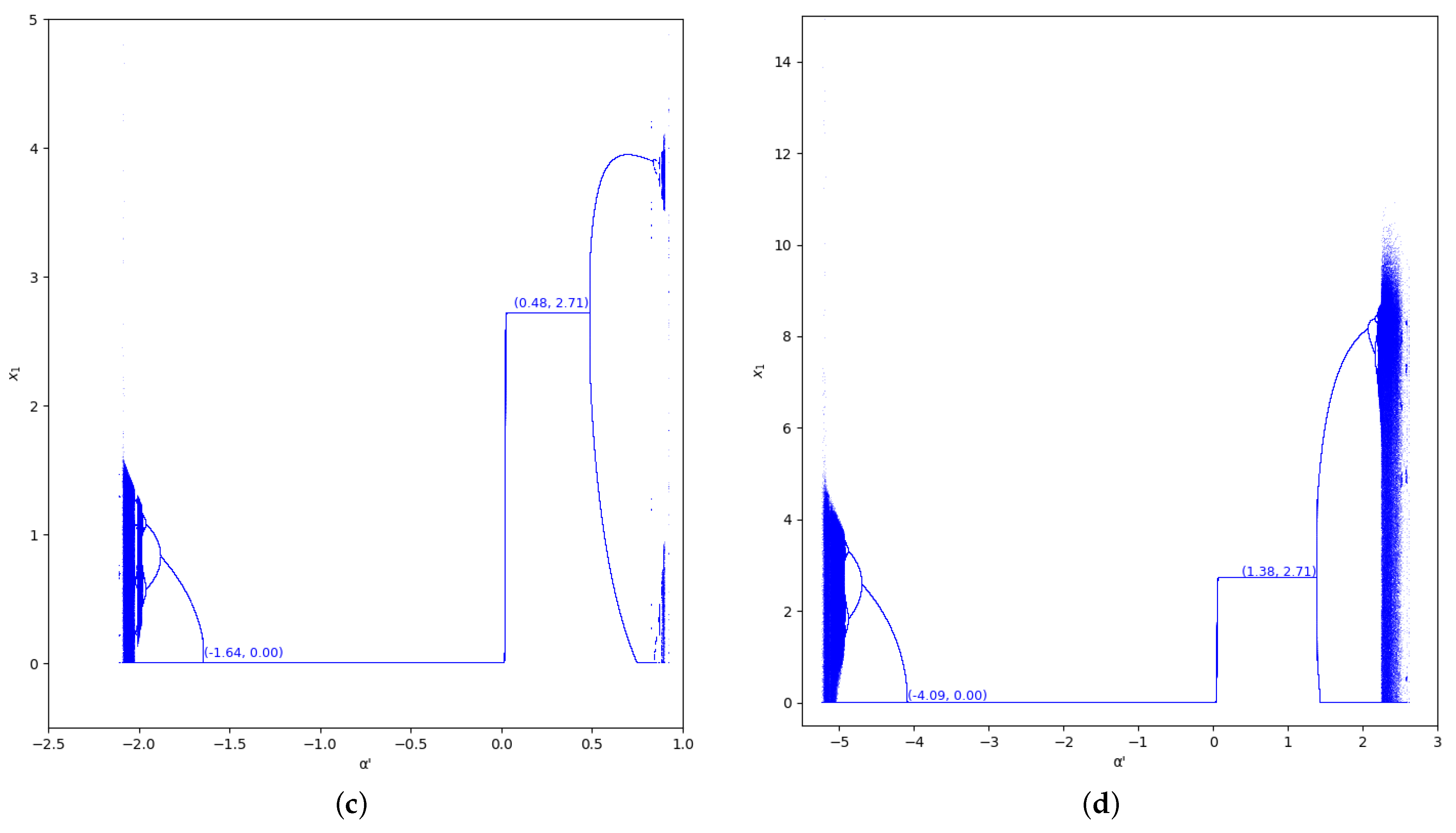
Figure 6.
Bifurcation diagrams of output of the first player as a function of with and in the zone (). (a) ; (b) ; (c) ; (d) .
Figure 6.
Bifurcation diagrams of output of the first player as a function of with and in the zone (). (a) ; (b) ; (c) ; (d) .
Figure 7.
Stability region for () in the absence of memory. The area with no economic sense is shaded in blue, that is, when and .
Figure 7.
Stability region for () in the absence of memory. The area with no economic sense is shaded in blue, that is, when and .
Figure 8.
Stability region for () and different values of (0, 0.2, 0.5, and 0.8). The vertical line is represented because this value and are the values used in the bifurcation diagrams. The area with no economic sense is shaded in blue, that is, when and .
Figure 8.
Stability region for () and different values of (0, 0.2, 0.5, and 0.8). The vertical line is represented because this value and are the values used in the bifurcation diagrams. The area with no economic sense is shaded in blue, that is, when and .
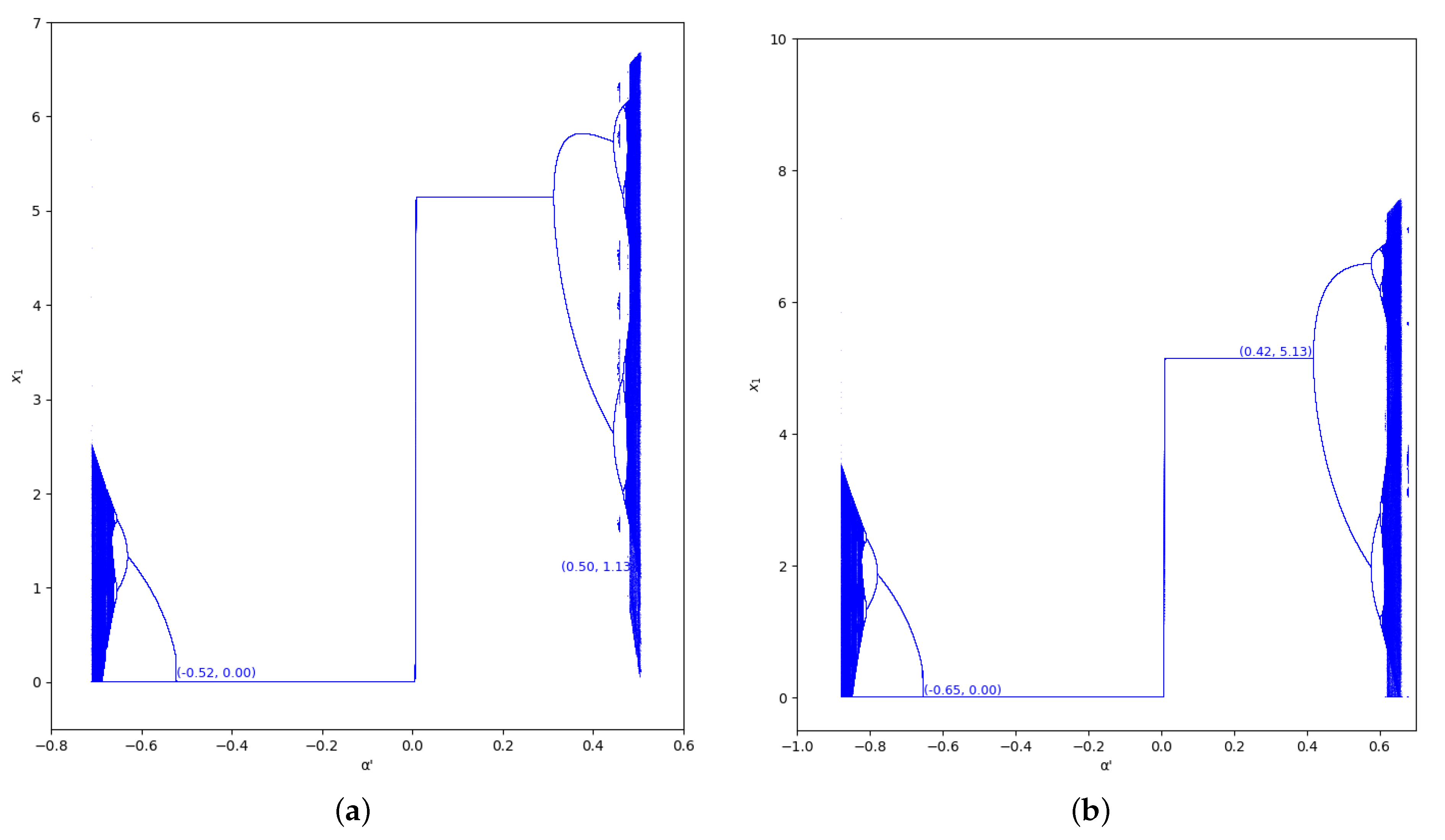
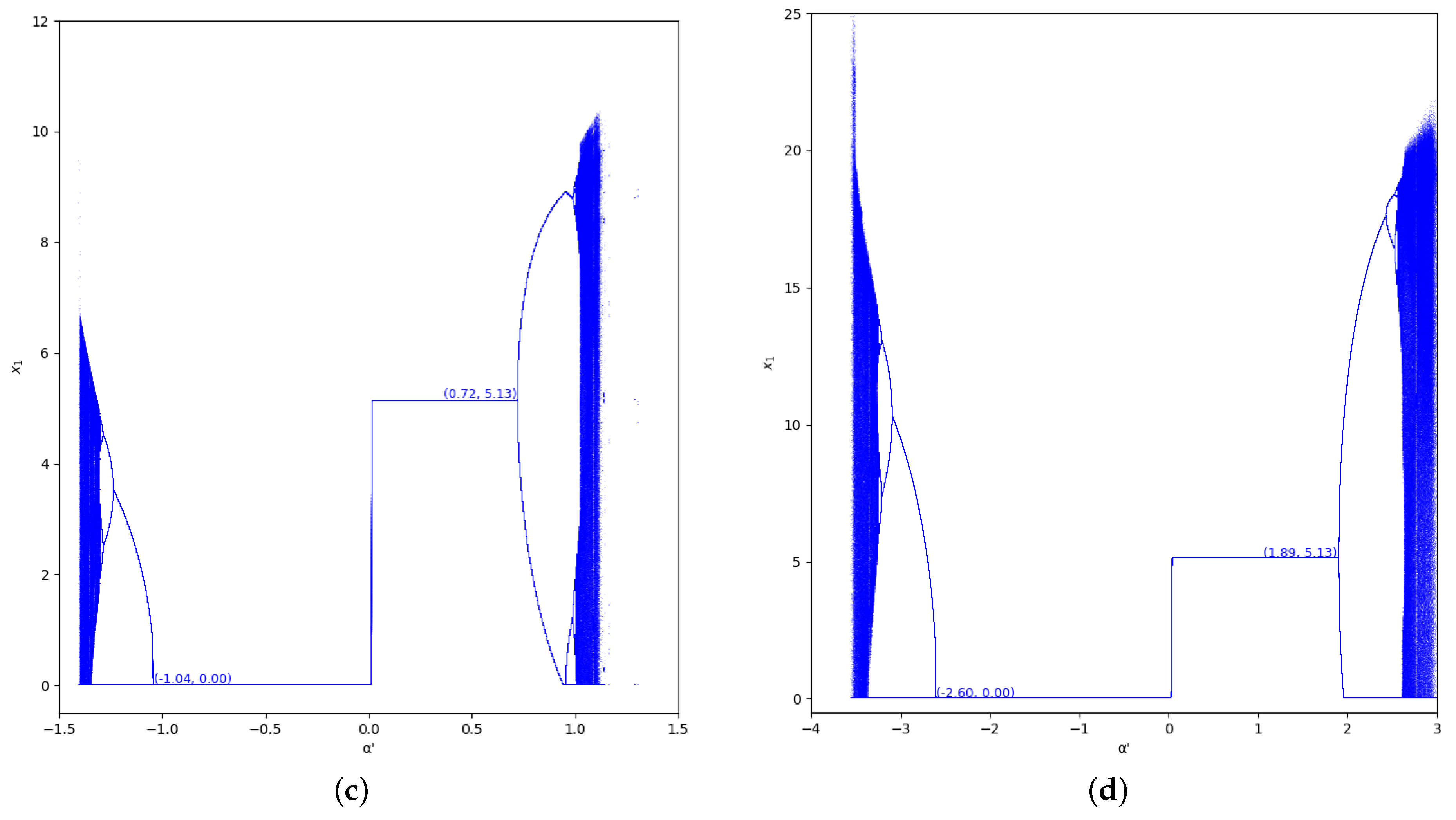
Figure 9.
Bifurcation diagrams of output of the first player as a function of with and in the zone (). (a) ; (b) ; (c) ; (d) .
Figure 9.
Bifurcation diagrams of output of the first player as a function of with and in the zone (). (a) ; (b) ; (c) ; (d) .
Figure 10.
Bifurcation diagrams of output of the first player as a function of with and in the zone (). (a) ; (b) ; (c) ; (d) .
Figure 10.
Bifurcation diagrams of output of the first player as a function of with and in the zone (). (a) ; (b) ; (c) ; (d) .
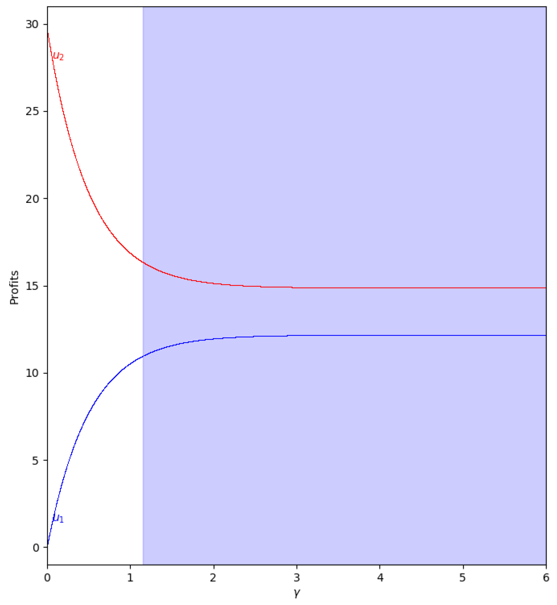
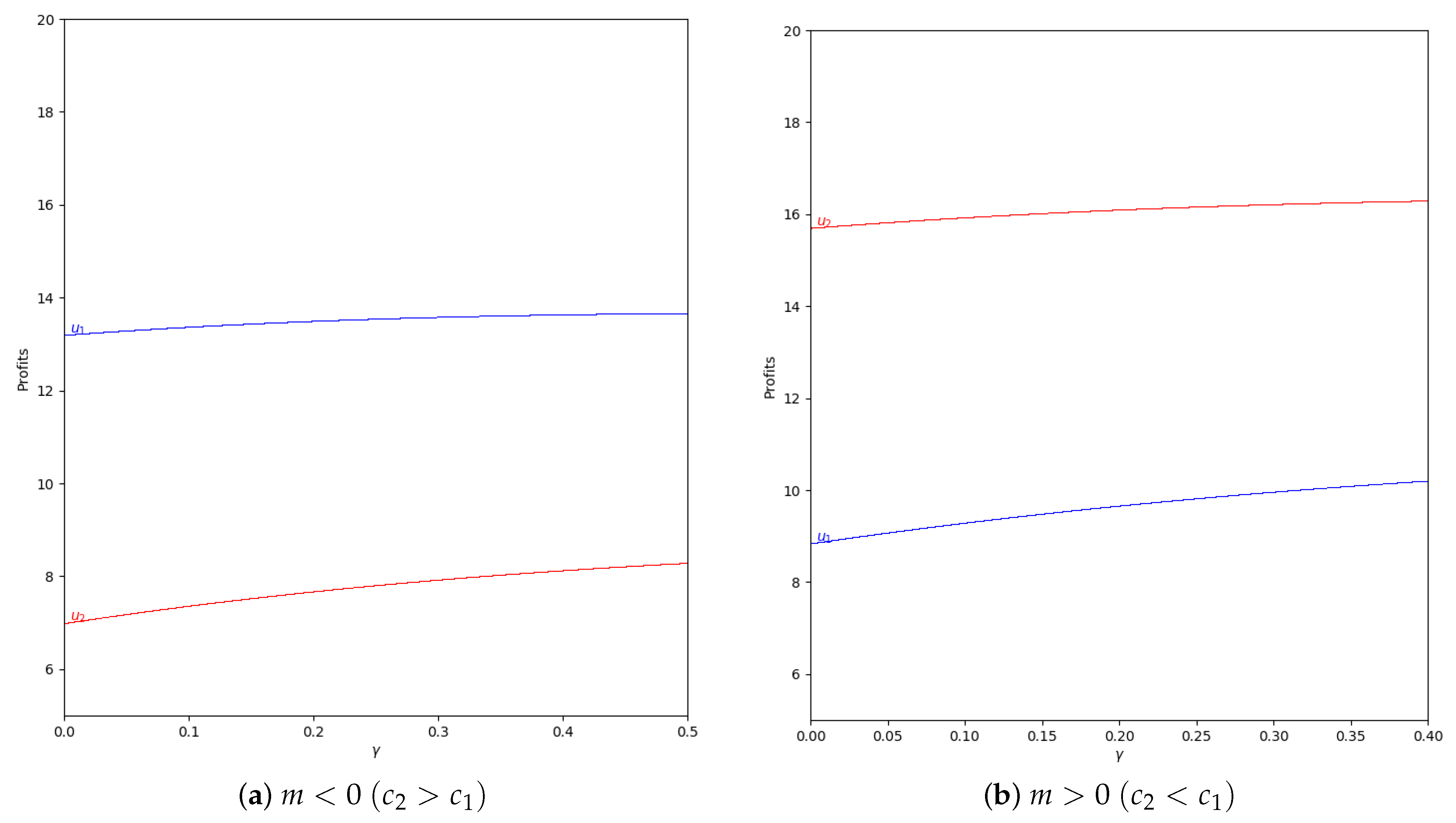
Figure 11.
Quantum profits of the two firms (
in blue and
in red) as a function of
(degree of quantum entanglement) with
(without memory) and
=0 (speed of adjustment is zero, therefore
) in the zone
(
) with initial value of
. The point where
is when
, but according to Equation (
47),
to have economic meaning.
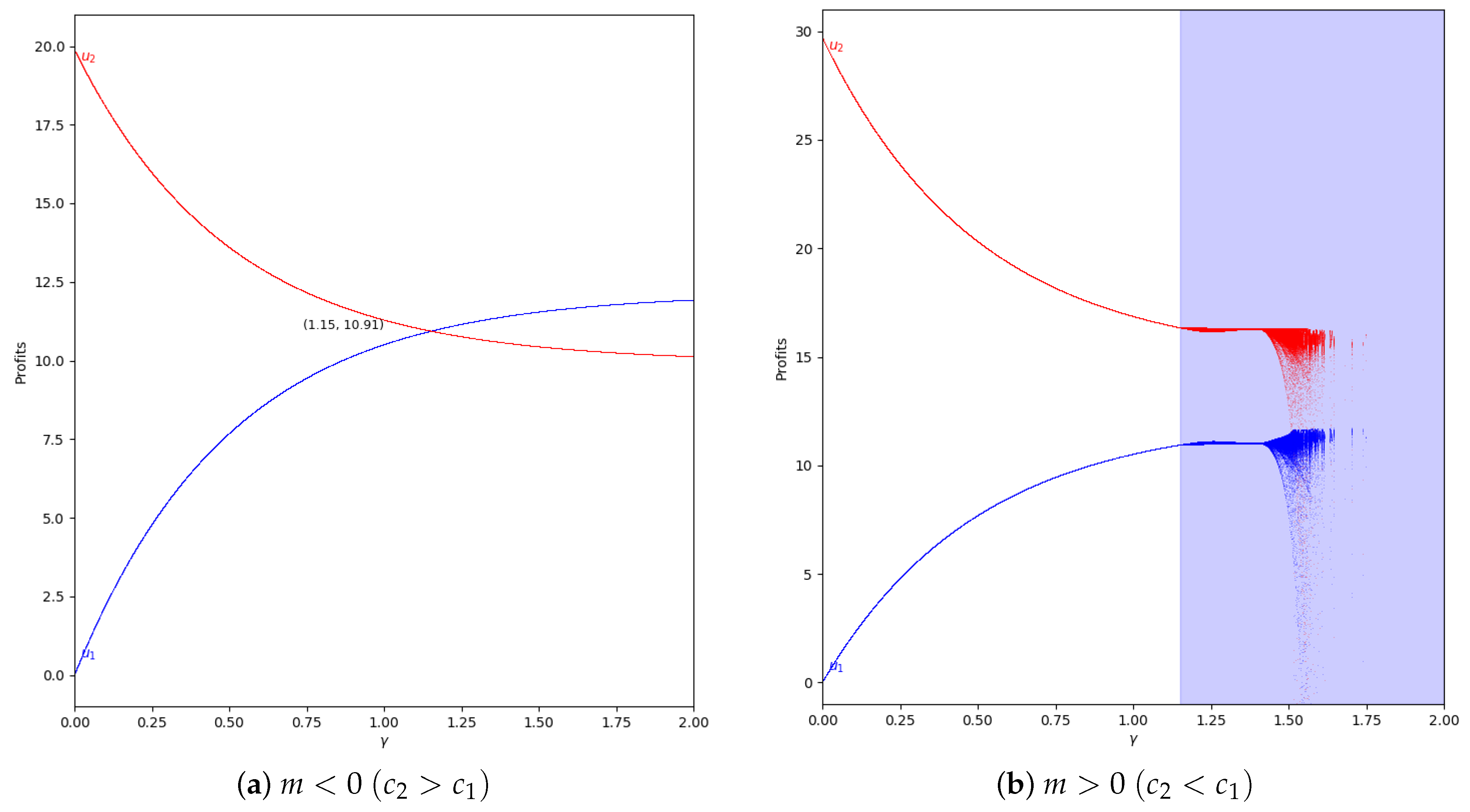
Figure 12.
Quantum profits of the two firms (
in blue and
in red) as a function of
(degree of quantum entanglement) with
(without memory) and
=0 (speed of adjustment is zero, therefore
) in the zone
(
) with initial value of
. When
the game has economic meaning according to Equation (
45).
Figure 12.
Quantum profits of the two firms (
in blue and
in red) as a function of
(degree of quantum entanglement) with
(without memory) and
=0 (speed of adjustment is zero, therefore
) in the zone
(
) with initial value of
. When
the game has economic meaning according to Equation (
45).
Figure 13.
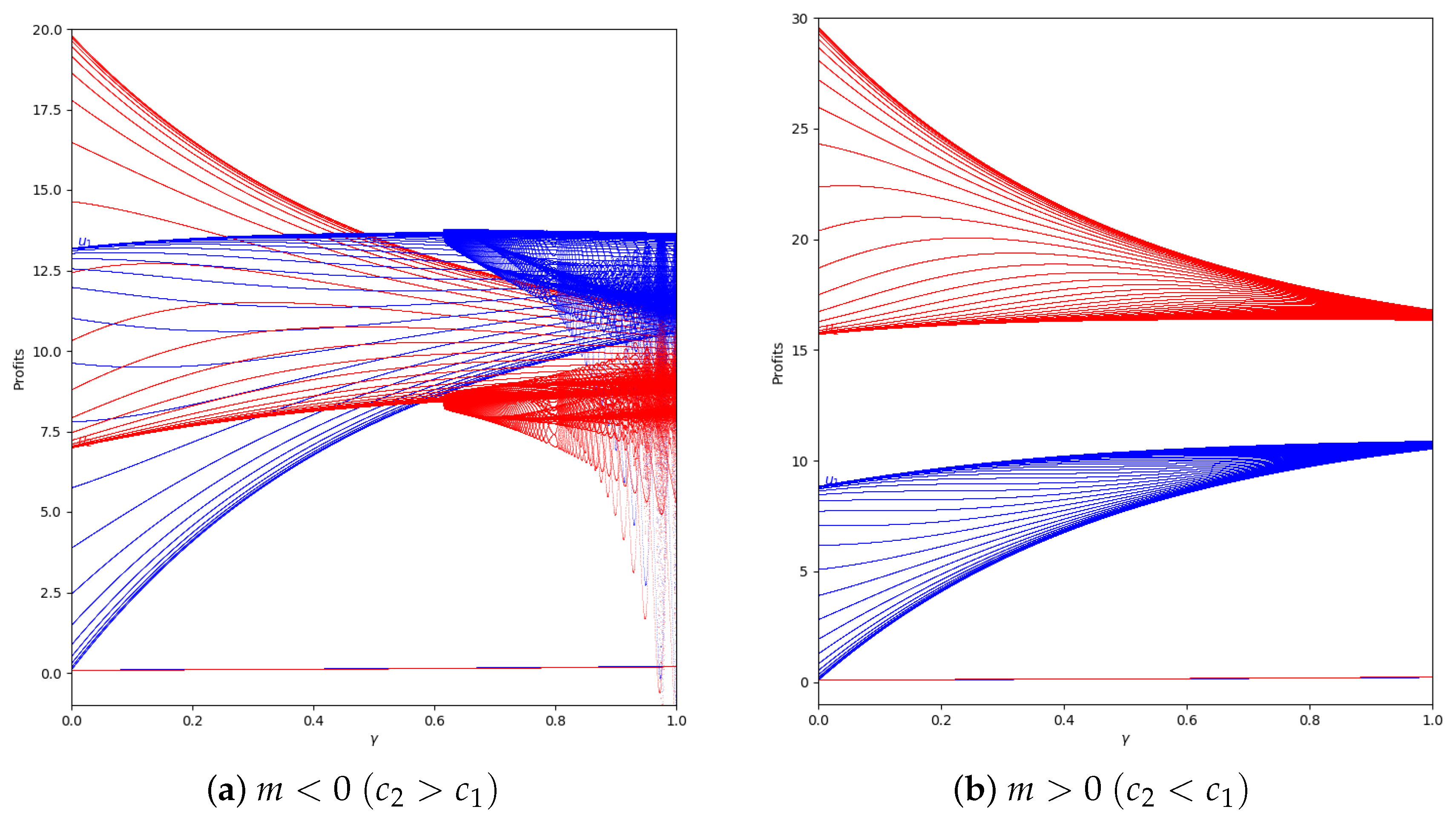
Quantum profits of the two firms ( in blue and in red) as a function of (degree of quantum entanglement) with (without memory) and = 0.2 (speed of adjustment): (a) in the zone (, ) and (b) in the zone (, ), with initial value of .
Figure 13.
Quantum profits of the two firms ( in blue and in red) as a function of (degree of quantum entanglement) with (without memory) and = 0.2 (speed of adjustment): (a) in the zone (, ) and (b) in the zone (, ), with initial value of .
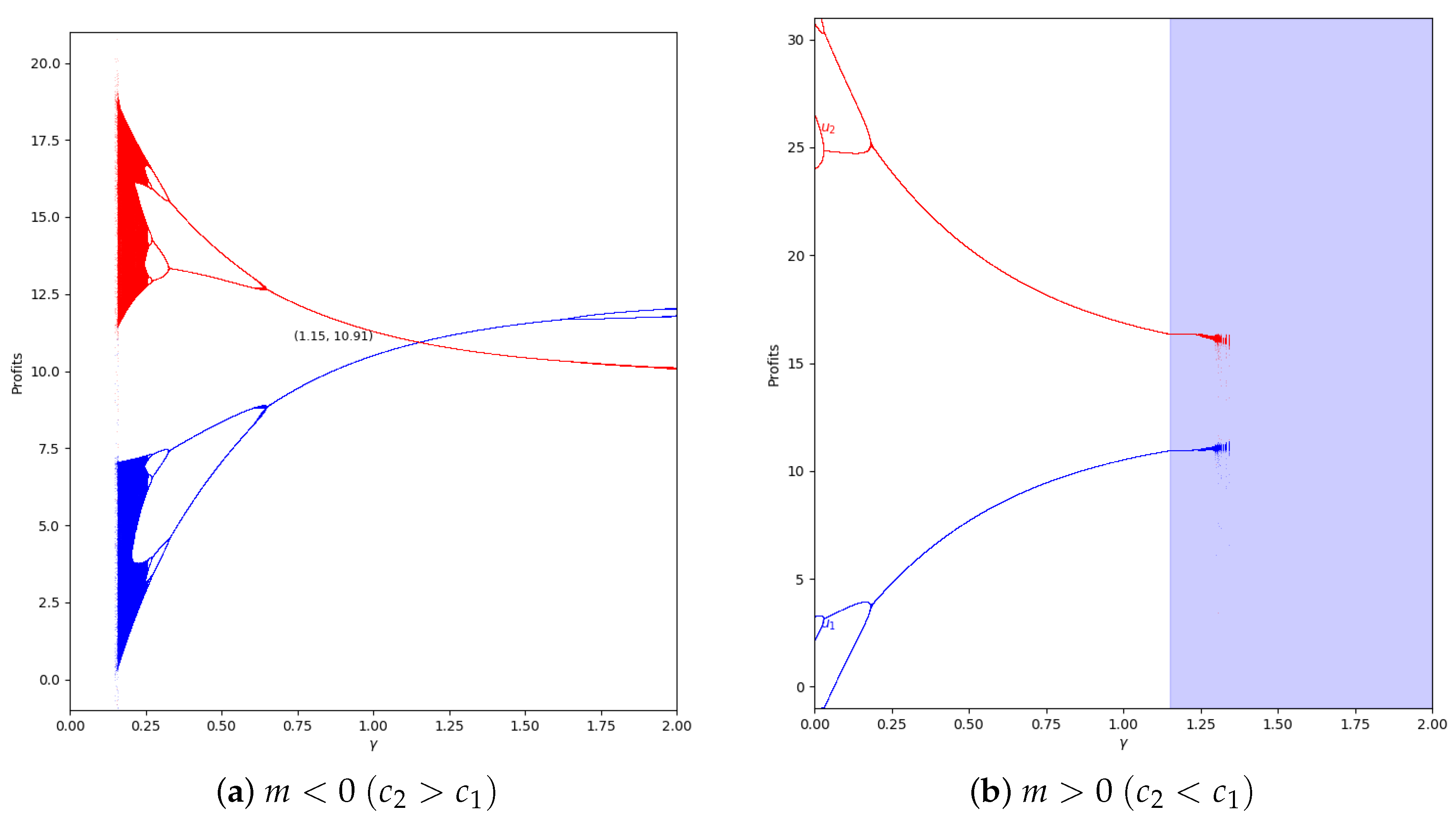
Figure 14.
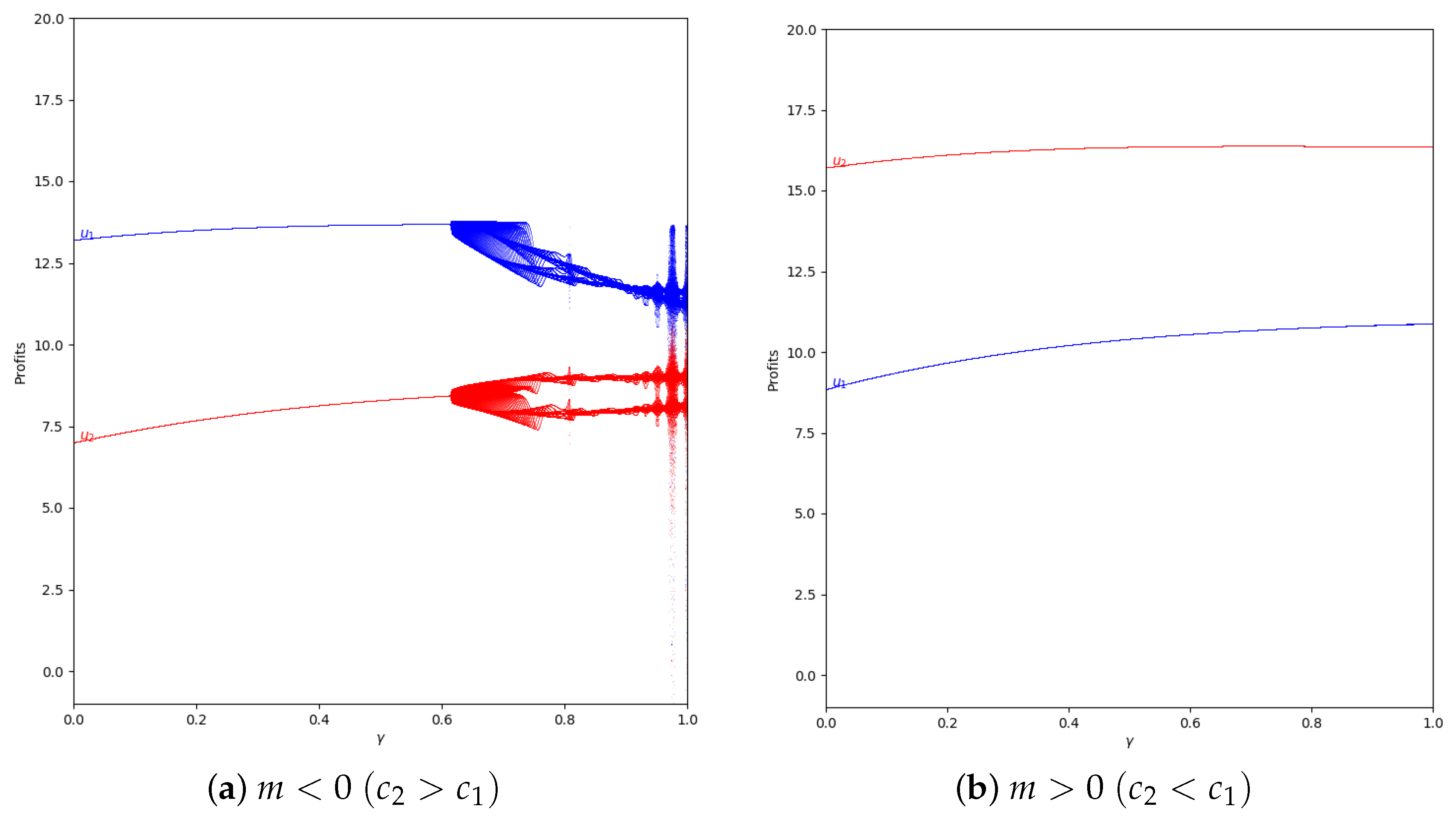
Quantum profits of the two firms ( in blue and in red) as a function of (degree of quantum entanglement) with (without memory), = 0.2 (speed of adjustment), and without the first 50 iterations: (a) in the zone () and (b) in the zone (), with initial value of .
Figure 14.
Quantum profits of the two firms ( in blue and in red) as a function of (degree of quantum entanglement) with (without memory), = 0.2 (speed of adjustment), and without the first 50 iterations: (a) in the zone () and (b) in the zone (), with initial value of .
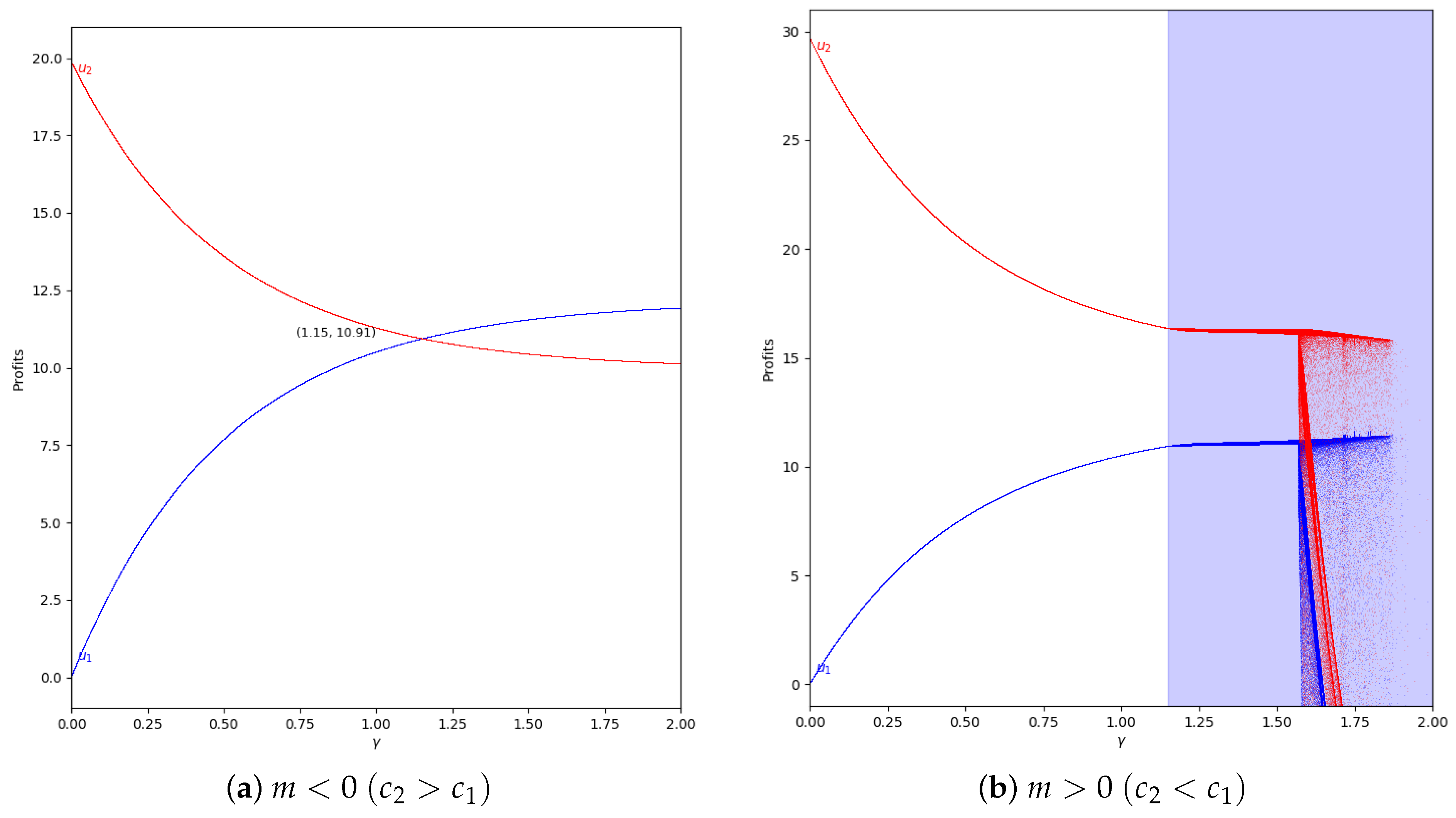
Figure 15.
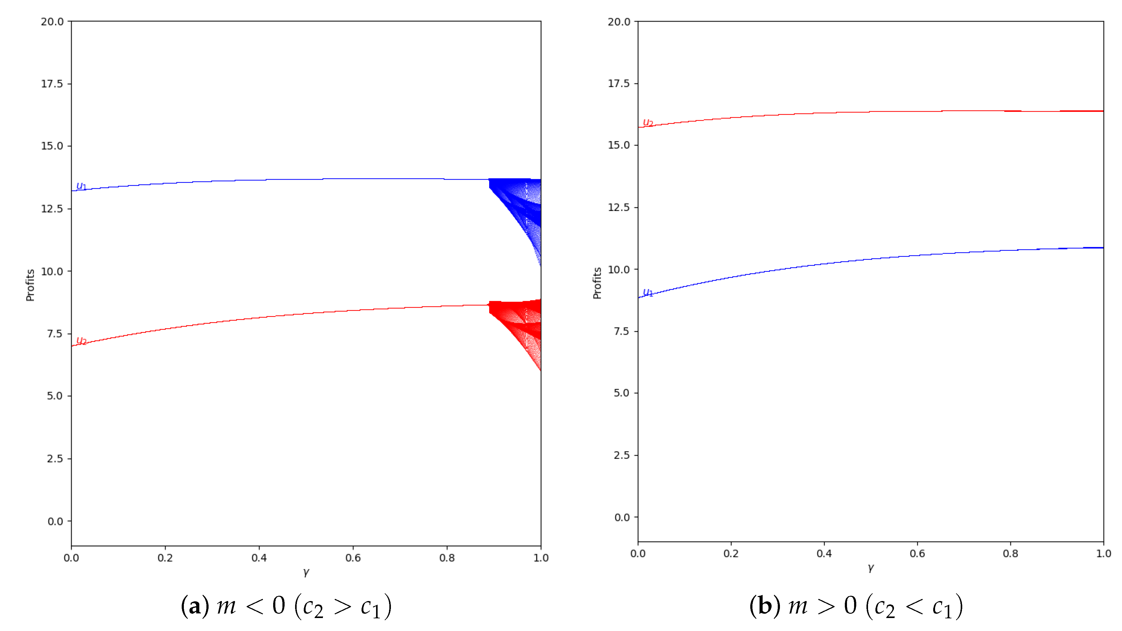
Quantum profits of the two firms ( in blue and in red) as a function of (degree of quantum entanglement) with (with memory), = 0.2 (speed of adjustment), and without the first 50 iterations: (a) in the zone () and (b) (), with initial value of .
Figure 15.
Quantum profits of the two firms ( in blue and in red) as a function of (degree of quantum entanglement) with (with memory), = 0.2 (speed of adjustment), and without the first 50 iterations: (a) in the zone () and (b) (), with initial value of .
Figure 16.
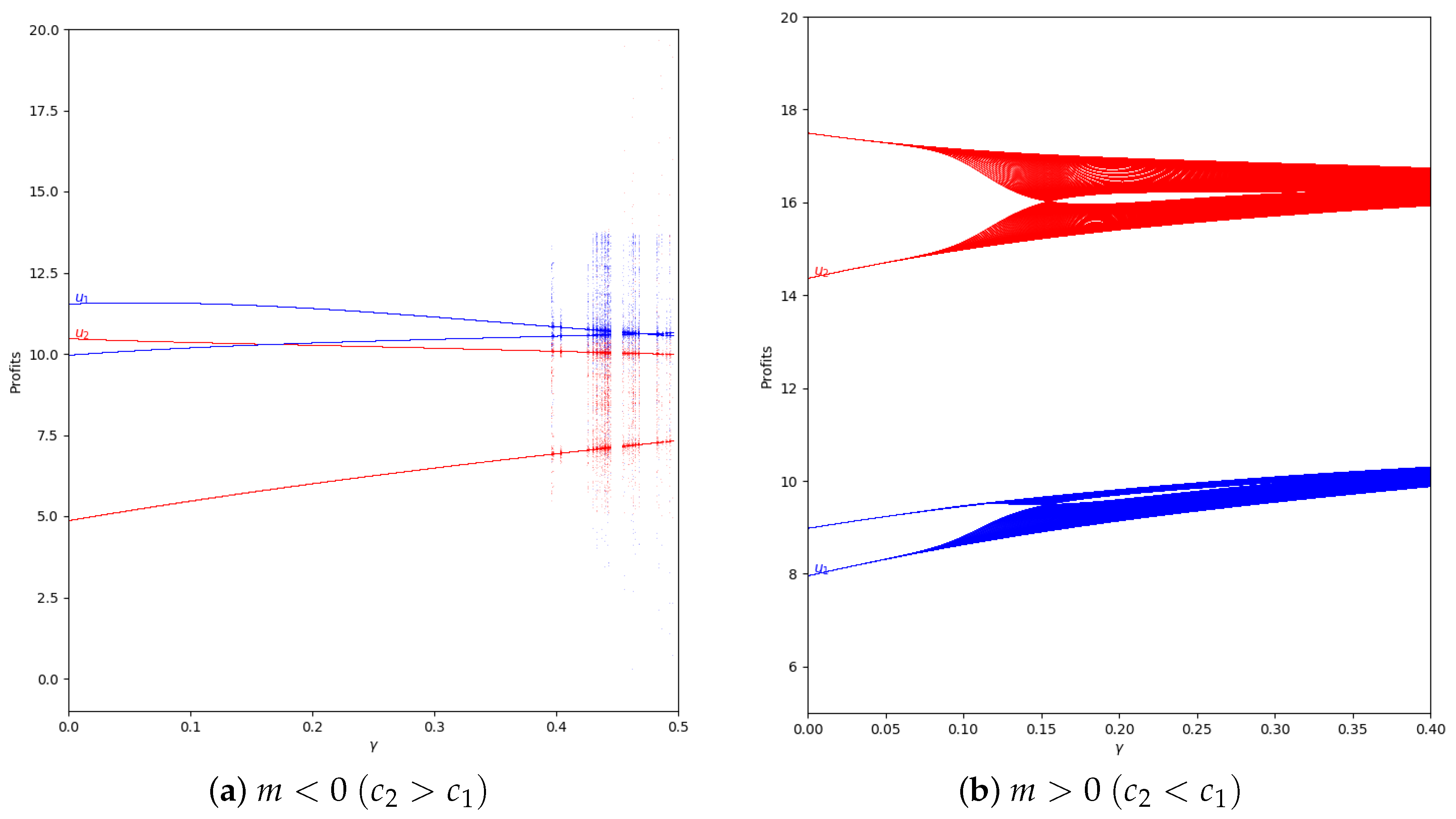
Quantum profits of the two firms ( in blue and in red) as a function of (degree of quantum entanglement) with (without memory), = 0.4 (speed of adjustment), and without the first 50 iterations: (a) in the zone () and (b) (), with initial value of .
Figure 16.
Quantum profits of the two firms ( in blue and in red) as a function of (degree of quantum entanglement) with (without memory), = 0.4 (speed of adjustment), and without the first 50 iterations: (a) in the zone () and (b) (), with initial value of .
Figure 17.
Quantum profits of the two firms ( in blue and in red) as a function of (degree of quantum entanglement) with (with memory), = 0.4 (speed of adjustment), and without the first 100 iterations: (a) in the zone () and (b) (), with initial value of .
Figure 17.
Quantum profits of the two firms ( in blue and in red) as a function of (degree of quantum entanglement) with (with memory), = 0.4 (speed of adjustment), and without the first 100 iterations: (a) in the zone () and (b) (), with initial value of .
Figure 18.
Quantum profits of the two firms (
in blue and
in red) as a function of
(degree of quantum entanglement) with
(without memory) and
= −0.2 (speed of adjustment): (
a) in the zone
(
) and (
b) in the zone
(
,
), with initial value of
. Regarding Equation (
50), in
, when
all values of
are valid, but when
, only the values of
are valid according to Equation (
45).
Figure 19.
Quantum profits of the two firms (
in blue and
in red) as a function of
(degree of quantum entanglement) with
(without memory) and
= −0.8 (speed of adjustment): (
a) in the zone
(
) and (
b) in the zone
(
,
), with initial value of
. Regarding Equation (
50), in
, when
all values of
are valid, but when
, only the values of
are valid according to Equation (
45).
Figure 20.
Quantum profits of the two firms (
in blue and
in red) as a function of
(degree of quantum entanglement) with
and
(speed of adjustment): (
a) in the zone
(
) and (
b) in the zone
(
), with initial value of
. Regarding Equation (
50), in
, when
, all values of
are valid, but when
, only the values of
are valid according to Equation (
45).


