Article

A Damping-Tunable Snap System: From Dissipative Hyperchaos to Conservative Chaos

by
Patinya Ketthong
and
Banlue Srisuchinwong
*
School of Information, Computer, and Communication Technology, Sirindhorn International Institute of Technology, Thammasat University, Pathum Thani 12120, Thailand
*
Author to whom correspondence should be addressed.
Entropy 2022, 24(1), 121; https://doi.org/10.3390/e24010121
Submission received: 16 December 2021 / Revised: 8 January 2022 / Accepted: 10 January 2022 / Published: 13 January 2022
(This article belongs to the Section Complexity)

Abstract

:
A hyperjerk system described by a single fourth-order ordinary differential equation of the form x = f ( x , x ¨ , x ˙ , x ) has been referred to as a snap system. A damping-tunable snap system, capable of an adjustable attractor dimension ( D L ) ranging from dissipative hyperchaos ( D L < 4 ) to conservative chaos ( D L = 4 ), is presented for the first time, in particular not only in a snap system, but also in a four-dimensional (4D) system. Such an attractor dimension is adjustable by nonlinear damping of a relatively simple quadratic function of the form A x 2 , easily tunable by a single parameter A. The proposed snap system is practically implemented and verified by the reconfigurable circuits of field programmable analog arrays (FPAAs).

1. Introduction

Studies of chaotic systems have received great attention due to many practical applications in science and technology [1,2,3]. Typically, a three-dimensional (3D) chaotic system is expressed by a set of three coupled first-order ordinary differential equations (ODEs), whereas a four-dimensional (4D) chaotic system is expressed by a set of four coupled first-order ODEs.
On the other hand, four successive time derivatives of displacement (x), for example, are known as velocity ( x ˙ ), acceleration ( x ¨ ), jerk ( x ) [4,5,6], and snap ( x or hyperjerk) [5], whereas a time derivative higher than the third is known as hyperjerk [7]. A chaotic jerk system is described by a single third-order ODE of the form x = f ( x ¨ , x ˙ , x ) , whereas a chaotic snap (or hyperjerk) system is described by a single fourth-order ODE of the form x = f ( x , x ¨ , x ˙ , x ) [7,8].
Chaos is typically measured by Lyapunov exponents ( L E s ) and a Lyapunov dimension ( D L ). The latter is alternatively known as a Kaplan–Yorke dimension ( D K Y ) or an attractor dimension [5]. The largest Lyapunov exponent ( L L E ) measures chaoticity [9], i.e., how much a system is sensitive to the initial conditions. A system will exhibit chaos if one L E is positive, but will exhibit hyperchaos if at least two L E s are positive [10]. On the contrary, the Lyapunov dimension or attractor dimension measures the complexity (strangeness) [9,11] of an attractor and is based on the calculation of all L E s . In addition, the negative sum of all L E s represents damping ( α ), the dissipation of energy from oscillations, of the form α = L i , where L i is the i-th L E , and therefore, damping plays an essential role not only in oscillations, but also in the value of an attractor dimension [5,12].
The attractor dimension ( D L ) also classifies whether chaos (or hyperchaos) in an n-dimensional, or n-th-order, system is dissipative ( D L < n) or conservative ( D L = n). Although not all undamped systems can exhibit chaos, conservative chaos (or hyperchaos) is however found in an undamped system where the average damping along the trajectories is zero ( α = 0 ) [5]. Conservative chaos (or hyperchaos) is therefore of special interest [13], but appears to be the minority of reported chaotic (or hyperchaotic) systems, whereas dissipative chaos (or hyperchaos) appears to be the majority. Although a transition between dissipative and conservative chaos is possible through adjustable damping for an adjustable attractor dimension, such a transition is however relatively rare. In particular, transitions ranging from dissipative hyperchaos to conservative chaos have never been reported.
In 3D chaotic flows, existing transitions from dissipative chaos ( D L < 3 ) to conservative chaos ( D L = 3 ) have been found in, for example, a damped, forced, pendulum [5] and in [14], of which the attractor dimension is adjustable to the maximum, i.e., D L 3 . On the contrary, such transitions to the maximum attractor dimension D L 4 have never been found in 4D or fourth-order (snap or hyperjerk) chaotic flows, although an attempt in a simple damping-tunable single-transistor-based chaotic snap circuit [12] has demonstrated its maximized attractor dimension (but D L 4 as D L = 3.28156 ) at its minimized damping (but α 0 as α 1 ).
Recently, field programmable analog arrays (FPAAs) [15], which offer reconfigurable circuits for analog signal processing, have been employed in implementing chaotic circuits and systems [16,17,18]. The advantages of FPAAs include that a mathematical model, such as a chaotic model, can be practically implemented by configurable circuits of FPAAs with ease, flexibility, reliability, and robustness. Such advantages greatly reduce the time and costs of a prototype.
In this paper, a new damping-tunable snap (hyperjerk) system capable of exhibiting conservative chaos, dissipative chaos, and dissipative hyperchaos is proposed. In addition, transitions ranging from dissipative hyperchaos to conservative chaos are demonstrated for the first time, especially not only in a snap system, but also in a 4D system. Its dynamical properties were investigated. Circuits for the new snap system were implemented through the use of FPAAs, which allowed us to verify its dynamical properties.

2. The Proposed Snap System

2.1. The General Form of a Snap System

Many simple hyperchaotic snap systems [7,19,20,21,22,23,24,25,26] have been presented in a single fourth-order ODE, which can be written in a general form as:
x = α x a 1 x ¨ a 2 x ˙ a 3 x a 4 g ( x ¨ , x ˙ , x )
where α is a damping coefficient [5,12] of the form:
α = a 0 f ( x )
a 0 , a 1 , a 2 , a 3 , a 4 are parameters, and f ( x ) and g ( x ¨ , x ˙ , x ) are nonlinear functions. As a result, the damping coefficient in (2) is a nonlinear damping coefficient. Table 1 compares such existing hyperchaotic snap systems [7,19,20,21,22,23,24,25,26] and shows that they do not exhibit conservative chaos, where ( A 1 to A 8 ) are tuning parameters and ( B 0 to B 7 ), C 8 , ( E 1 to E 8 ), ( F 5 , F 6 , F 8 ), and ( G 6 , G 8 ) are constants, all of which are not equal to one. Note that B 9 is described in Section 2.4.

2.2. A New Damping-Tunable Snap System

Further studies through individual simulations showed that existing systems [7,19,20,21,22,23,24,25] based on (1) continue to exhibit hyperchaos for positive values of a 2 , whereas the existing nonlinear function f ( x ) = x 4 can be alternatively replaced by a new simpler nonlinear function f ( x ) = x 2 . In particular, additional studies revealed that conservative chaos is possible if the damping coefficient α = 0 and the parameter a 2 = 0 . Such studies led to a new single fourth-order ODE of the proposed snap system of the form:
x = A ( x 2 x + x ˙ ) B x ¨ | x ˙ | x
where A is a tuning parameter, B = 2.65 is a constant, f ( x ) = x 2 , and g ( x ¨ , x ˙ , x ) = | x ˙ | , as also included in Table 1. It can be noticed from Table 1 that the nonlinear function f ( x ) in (3) is a quadratic function of the form x 2 , whereas f ( x ) in existing systems [7,19,20,21,22,23,24,25] is a quartic function of the form x 4 . Although the system in [26] has f ( x ) = 1 , the function g ( x ¨ , x ˙ , x ) consists of many trigonometric functions that lead to difficulties in circuit implementation.
Based on (2) and Table 1, the damping coefficient in (3) is of the form:
α = A x 2
By tuning the parameter A, as will be shown later, the proposed snap system in (3) can exhibit not only dissipative hyperchaos, but also conservative chaos.
Equivalently, the damped snap system in (3) can be rewritten as a 4D damped dynamical system in a set of four coupled first-order ODEs of the form:
x ˙ = y y ˙ = z z ˙ = w w ˙ = A ( w x 2 + y ) 2.65 z | y | x
where the state variables are defined as:
x y z w = x x ˙ x ¨ x
By substituting x ˙ = 0 , y ˙ = 0 , z ˙ = 0 and w ˙ = 0 in (5), the corresponding equilibrium point in (5) is located at E 1 = ( x 0 , y 0 , z 0 , w 0 ) = ( 0 , 0 , 0 , 0 ) .

2.3. Snap-Based Dissipative Hyperchaos

The 4D damped dynamical system in (5) was numerically simulated by using the adaptive fourth-order Runge–Kutta (RK4) integration [27] with an adaptive step size Δ t 0.01 . Figure 1a,b, respectively, shows the Lyapunov dimension ( D L ) and the spectrum of L E s ( L 1 , L 2 , L 3 , L 4 ), ordered from large to small values, of (5) versus the parameter A from 0–0.5. The calculations of the spectrum of L E are based on the algorithm proposed by Wolf et al. [28]. An initial condition is ( x , y , z , w ) = ( 0.1 , 0.1 , 0.1 , 0.1 ) . To ensure that chaos and hyperchaos are neither transients nor numerical artifacts, the calculations of the Lyapunov dimension and L E s follow the orbit for a sufficiently large time of t = 10 8 .
As shown in Figure 1b, where A 0 and D L < 4 , the damped snap system in (3) can exhibit not only snap-based dissipative chaos, but also snap-based dissipative hyperchaos. The latter exists for A ( 0.22 , 0.35 ) .
For system stability, the corresponding Jacobian matrix is written as:
J 1 = 0 1 0 0 0 0 1 0 0 0 0 1 2 A w x A s g n ( y ) 2.65 A x 2
For example, at A = 0.275 , where the dissipative hyperchaos exists, the eigenvalues are λ 1 , 2 = 0.0759 ± 1.4996 i and λ 3 , 4 = 0.0759 ± 0.6617 i at the equilibrium point E 1 = ( 0 , 0 , 0 , 0 ) , and therefore, E 1 is a spiral saddle equilibrium with index 2.
For the dissipative chaos and hyperchaos in the damped snap systems in (3), the (positive) damping coefficient in (4) refers to the (negative) rate of a phase space expansion [5,12,28] of the form:
α = · F = T r ( J ) = i = 1 4 L i
where F is the flow in (5), · F is the time-averaged divergence of the flow F, T r ( J ) is the trace of the Jacobian matrix J 1 in (7) averaged along the trajectory, and L i is the i-th L E . As a result, the damped snap system in (3) is a dissipative system.

2.4. Snap-Based Conservative Chaos

In addition to the snap-based dissipative hyperchaos, the proposed snap system in (3) is capable of exhibiting snap-based conservative chaos at A = 0 where D L = 4 , as shown in Figure 1a, and therefore, the damped snap system in (3) is reduced to an undamped snap system of the form:
x = 2.65 x ¨ | x ˙ | x
where the damping coefficient in (4) is α = 0 . The resulting undamped snap system in (9) appears to be in a similar form as an existing undamped snap system of the form [8]:
x = B 9 x ¨ ± | x ˙ | x
where B 9 = 2.525 , as also included in Table 1. This is the first time, especially in a snap system and a 4D system, that transitions between conservative chaos in (9) and dissipative hyperchaos in (3) can be realizable.
Equivalently, the undamped snap system in (9) can be rewritten as a 4D undamped dynamical system of the form:
x ˙ = y y ˙ = z z ˙ = w w ˙ = 2.65 z | y | x
The corresponding Jacobian matrix is of the form:
J 2 = 0 1 0 0 0 0 1 0 0 0 0 1 1 s g n ( y ) 2.65 0
At A = 0 , where the conservative chaos exists, the eigenvalues are λ 1 , 2 = 0 ± 1.4919 i and λ 3 , 4 = 0 ± 0.6703 i at the equilibrium point E 2 = ( 0 , 0 , 0 , 0 ) , and therefore, E 2 is a nonhyperbolic equilibrium, of which at least one eigenvalue has a zero real part. In particular, all eigenvalues of E 2 have no real part. Such eigenvalues lie on the imaginary axis with the absence of real parts for conservative chaos.
For the conservative chaos in the undamped systems in (9), the damping coefficient in (8) becomes zero, where F is the flow in (11), and T r ( J ) is the trace of the Jacobian matrix J 2 in (12) averaged along the trajectory. As a result, the phase space of the systems in (9) is neither compressible nor expandable, and therefore, the undamped snap system in (9) is a conservative system.
A non-geometric integrator such as the RK4 integrator may affect the behavior of chaotic systems, especially of conservative systems, as non-geometric integrators may not fully preserve the properties of the continuous prototype in discrete calculations [29]. In an attempt to avoid possible dissipation appearing from such numerical methods, both the trace of the Jacobian matrix averaged along the trajectories and the summation of all LEs in (8) have been closely monitored to ensure the conservation of energy. The former always results in zero, whereas the latter is taken as zero if | i L i | < 0.001 , enabling the estimated uncertainty of less than 0.001 | i L i | .

2.5. Tunable Damping: From Dissipative Hyperchaos to Conservative Chaos

Substituting the damping coefficient in (4) into (8) yields:
α = A x 2 = i = 1 4 L i
It can be observed from (13) that changes in the parameter A result in not only changes in the Lyapunov dimension (attractor dimension D L ), as shown in Figure 1a, but also changes in the damping coefficient ( α ), as shown in Figure 2. In particular, Figure 3 depicts the Lyapunov dimension (attractor dimension D L ) in Figure 1a versus the damping coefficient ( α ) in Figure 2.
In a similar manner to the damping coefficient ( α ) in (8), it is evident from Figure 3 that a decrease in damping, e.g., from α = 0.2655 to 0.0, allows a phase space expansion with the tendency of an increase in the Lyapunov dimension (i.e. attractor dimension), e.g., from D L = 1.0 to 4.0. In particular, the minimized damping at α = 0.0 yields the maximized attractor dimension at D L = 4.0. Such an expansion demonstrates transitions, ranging from dissipative hyperchaos to conservative chaos, for the first time, in particular in a snap system and in a 4D system.

2.6. Multistability and Coexisting Attractor

Figure 4 illustrates the basins of attraction of (11) in red and purple areas of conservative chaos and periodic oscillations, respectively, on an ( x , y ) plane, where z = w = 0 . The equilibrium point is a blue dot at ( x , y ) = ( 0 , 0 ) . The system (11) therefore exhibits multistability and two coexisting oscillations. Figure 5 shows two examples of asymmetric coexisting attractors, of which the initial conditions are ( 0.01 , 0 , 0 , 0 ) and ( 0.01 , 0 , 0 , 0 ) for conservative chaos and periodic oscillations, respectively.

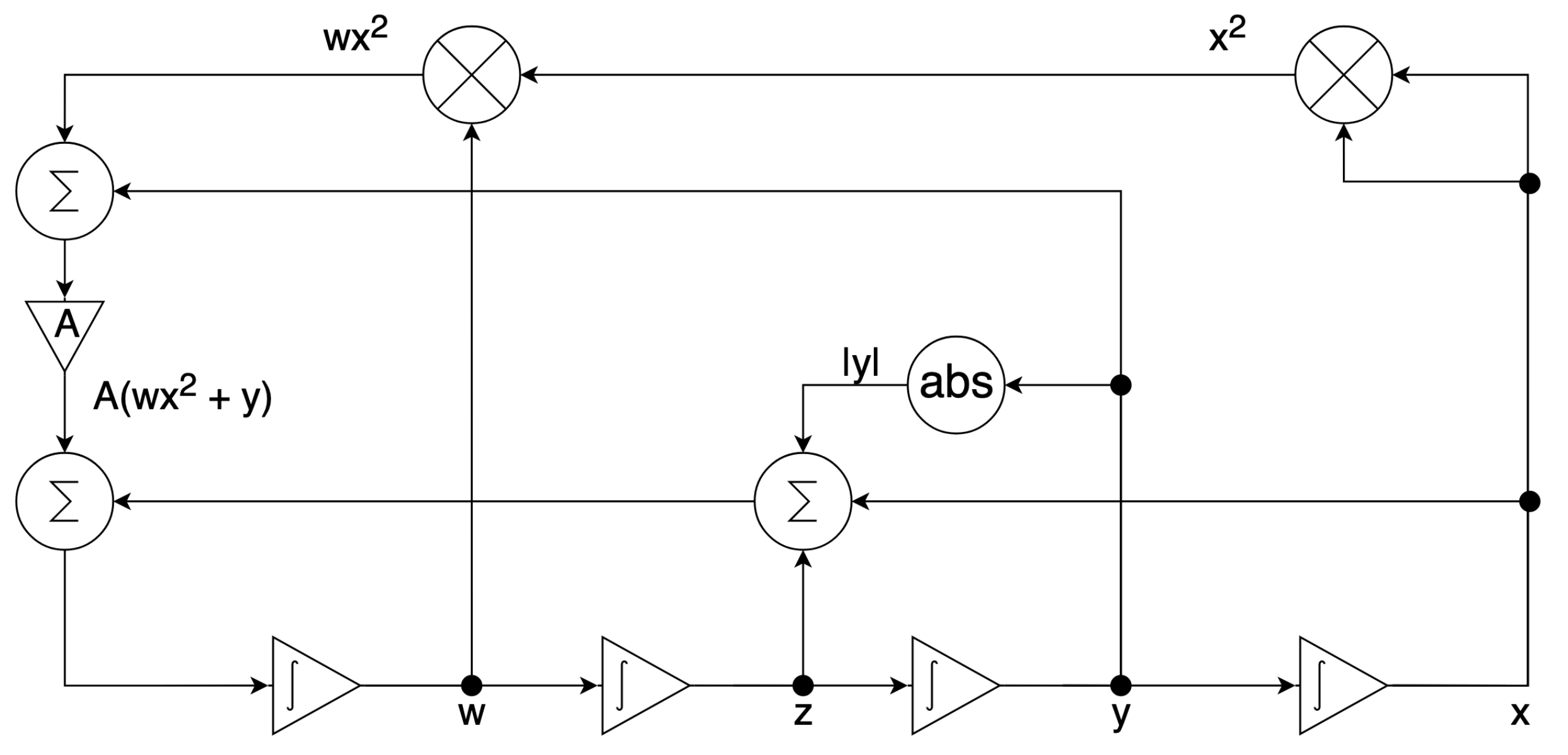
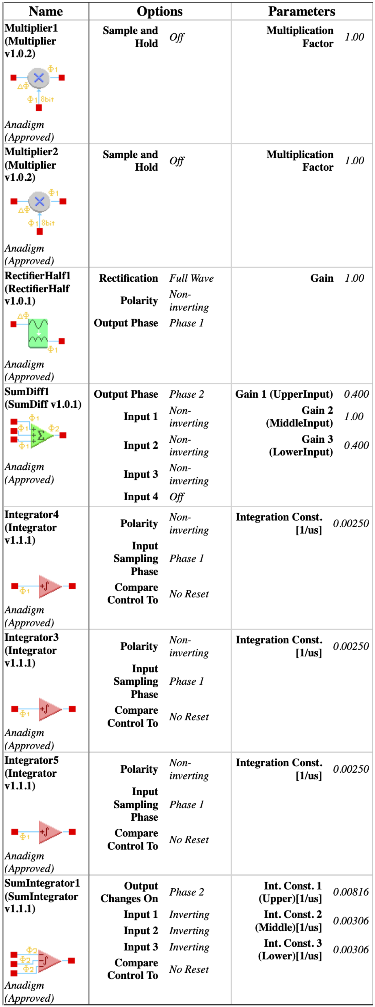
3. FPAA-Based Circuit Implementation

It is customary that the behavior of a newly proposed chaotic model can be verified by a proof through its analog circuit implementation such that properties such as numerical trajectories of the simulated model can be directly compared to oscilloscope-trace trajectories of its real experimental circuit for verification. In particular, it is increasingly customary that field programmable analog arrays (FPAAs) are used for such an analog circuit implementation.
FPAAs are programmable integrated circuits that enable flexible and rapid prototyping of analog circuits using configurable analog modules (CAMs). In addition, FPAAs provide efficient and economical solutions to design analog dynamical systems with increased reliability. Two (or four) FPAA chips, each of which is AN231E04, are on an Anadigm DualApex (or QuadApex) Development Board and are programmed and designed for circuits by AnadigmDesigner2 [15].
To avoid possible confusions, it should be emphasized that an FPAA is totally different from an field programmable gate array (FPGA). An FPAA is based on programmable analog building blocks, e.g., integrators, filters, and switched-capacitor circuits, whereas an FPGA is based on configurable logic modules or look-up tables and does not involve analog building blocks. In particular, FPAAs are fully programmable analog circuits, whereas FPGAs are programmable digital circuits. Although an FPGA may require a procedure such as a linearization method to convert differential equations to the binary or digital terms for the implementation on an FPGA [30], an FPAA does not at all require this.
Typically, the design procedure of FPAAs can be divided into two parts. The first part involves mathematical models, numerical simulations, and scaling processes. The latter may be required if the amplitude of the chaotic signals is larger than the supply voltage of the FPAAs. The second part involves the system being able to be modeled by CAMs, which are programmed into FPAA chips. If there are any mismatches between the numerical simulations from the first part and the experimental results from the second part, such mismatches may be eliminated by modifying the parameters inside the CAMs.
As an integrator of FPAAs is scaled by a constant k = 1 / τ , where τ is the time constant of the integrator, e.g., if τ = 0.4 ms, then k = 0.0025 (1/us), the scaling processes of the snap system in (3) are required. In other words, the system in (5) is scaled to be:
x ˙ = k 1 y y ˙ = k 2 z z ˙ = k 3 w w ˙ = k 4 [ A ( w x 2 + y ) 2.65 z | y | x ]
where the scaling factors are k 1 = k 2 = k 3 = 0.0025 (1/us) and k 4 = 0.00306 (1/us).
The scaled system in (14) is implemented by the configurable circuits of the first chip (FPAA1) for the dissipative hyperchaos with A 0 , as shown in Figure 6, whereas (14) is implemented by the configurable circuits of the second chip (FPAA2) for the conservative chaos with A = 0 , as shown in Figure 7. Each configurable circuit consists of four integrator blocks and a full-wave rectifier block. The latter is for the absolute function. The state variables x , y , z , and w are the outputs of individual integrator blocks.
For dissipative hyperchaos, the nonlinear damping coefficient ( α ) is implemented by additional circuits using two multiplier blocks and a summing block, as shown in Figure 6. For values of the scaling factors in (14), Figure 8 and Figure 9 [15] show the parameters and time constants of CAMs for the first (FPAA1) and second (FPAA2) chips, respectively. In addition, clock-A of the individual components is configured by default at 250 kHz, whereas clock-B is additionally required by the multipliers to be 16-times that of clock-A at 4 MHz.

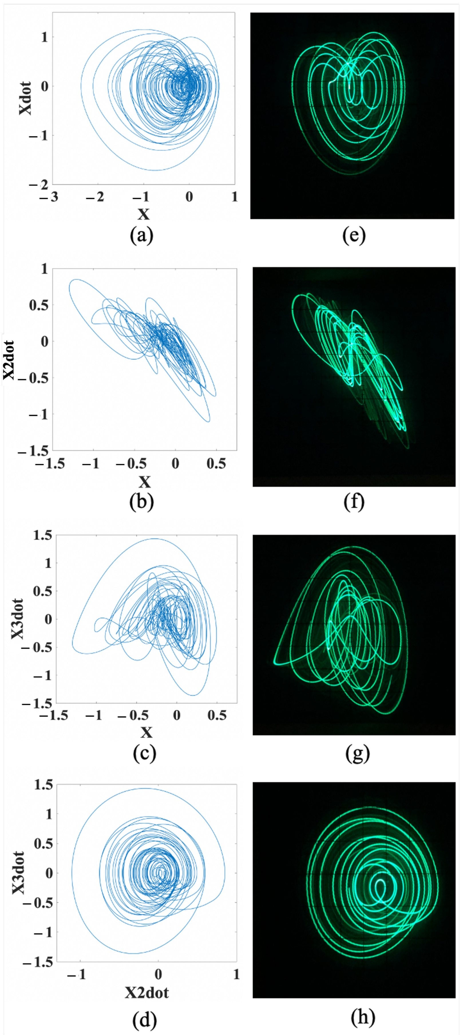
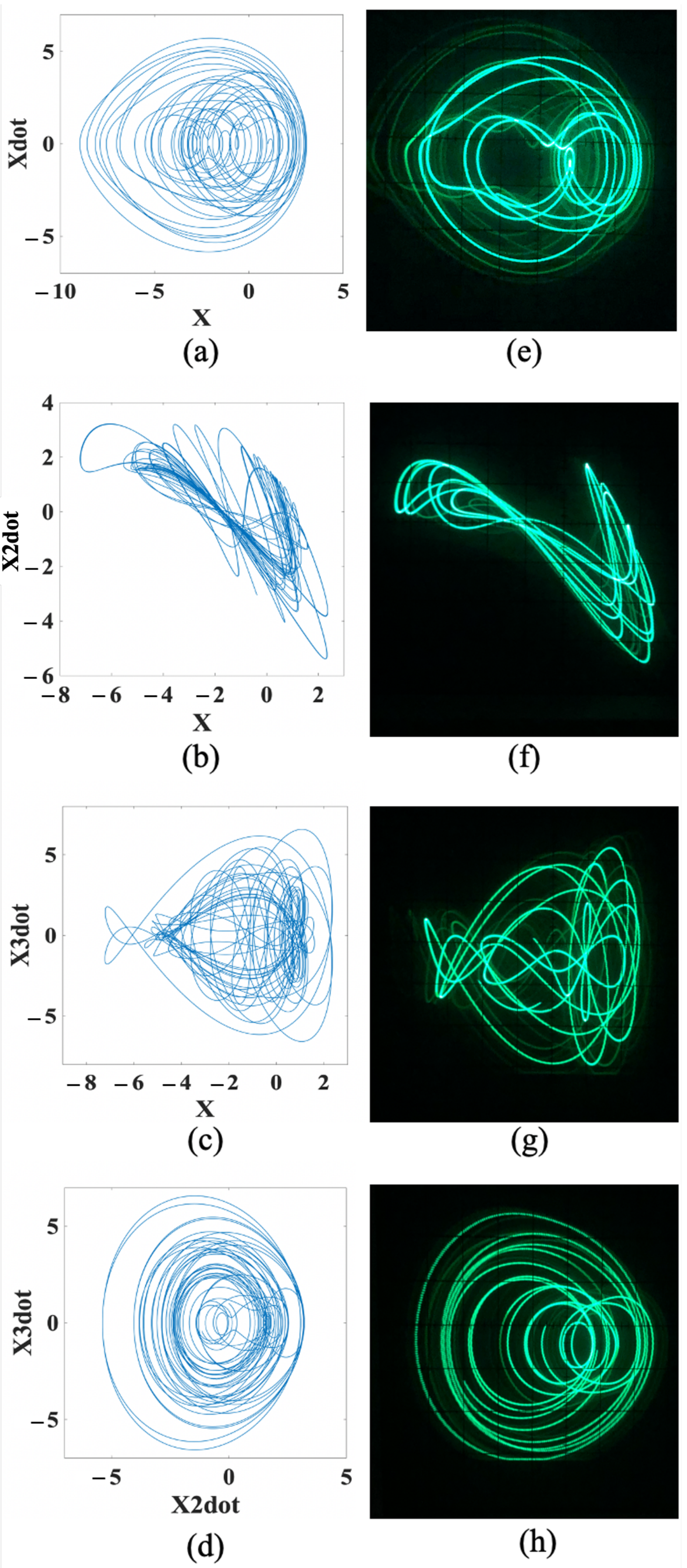
4. Numerical and Experimental Results

For the proposed snap system, the numerical trajectories of the simulated model in Section 2 and oscilloscope-trace trajectories of FPAA-based real experiments in Section 3 are compared in this section. The oscilloscope-trace trajectories are readily available from the FPAAs and, therefore, can be directly measured by an analog oscilloscope (e.g., GW-Instek GOS-620) without the need for extra ADC or DAC circuits.
On the one hand, at A = 0.275 , for the snap-based dissipative hyperchaos, the numerical trajectories of the attractors are illustrated in Figure 10a–d, whereas the corresponding FPAA-based oscilloscope traces are shown in Figure 10e–h, on the (x, x ˙ ), (x, x ¨ ), (x, x ), and ( x ¨ , x ) planes, respectively.
On the other hand, at A = 0 , for the snap-based conservative chaos, the numerical trajectories of the attractors are illustrated in Figure 11a–d, whereas the corresponding FPAA-based oscilloscope traces are shown in Figure 11e–h, on the (x, x ˙ ), (x, x ¨ ), (x, x ), and ( x ¨ , x ) planes, respectively. It can be noticed from Figure 10 and Figure 11 that both the numerical results and FPAA-based experimental results are in good agreement.

5. Conclusions

A new damping-adjustable fourth-order hyperjerk (snap) system was proposed and capable of tunable nonlinear damping for an adjustable attractor dimension ( D L ), resulting in transitions ranging from dissipative hyperchaos with D L < 4 to conservative chaos with D L = 4 . Such transitions were demonstrated for the first time, in particular in either a snap system or a 4D system. The tunable nonlinear damping was based on a relatively simple quadratic function of the form A x 2 , conveniently adjustable by a single tuning parameter A. The experimental results were based on the reconfigurable circuits of FPAAs and corresponded to the numerical simulations.

Author Contributions

Conceptualization, P.K. and B.S.; Data curation, P.K.; Formal analysis, P.K. and B.S.; Funding acquisition, B.S.; Investigation, P.K. and B.S.; Methodology, P.K.; Project administration, B.S.; Resources, P.K. and B.S.; Software, P.K. and B.S.; Supervision, B.S.; Validation, B.S. All authors have read and agreed to the published version of the manuscript.

Funding

The first author received a scholarship from the Thailand Advanced Institute of Science and Technology-Tokyo Institute of Technology (TAIST-Tokyo Tech).

Institutional Review Board Statement

Not applicable.

Informed Consent Statement

Not applicable.

Data Availability Statement

Not applicable.

Acknowledgments

The authors are grateful to J. C. Sprott for his permission to use his software for the calculations of the spectrum of the Lyapunov exponents and to Wimol San-Um for his useful comments. The first author appreciates Thai-Nichi Institute of Technology for the permission to spend time for a graduate study at Thammasat University and for the use of the FPAA development board. The first author would like to express gratitude for the Thailand Advanced Institute of Science and Technology-Tokyo Institute of Technology (TAIST-Tokyo Tech) scholarship.

Conflicts of Interest

The authors declare no conflict of interest.

References

  1. Coumo, K.M.; Oppenheim, A.V. Circuit implementation of synchronized chaos with application to communications. Phys. Rev. E 1993, 71, 65–68. [Google Scholar] [CrossRef] [PubMed]
  2. Cho, K.; Miyano, T. Chaotic Cryptography Using Augmented Lorenz Equations Aided by Quantum Key Distribution. IEEE Trans. Circuits Syst. I Regul. Pap. 2014, 62, 478–487. [Google Scholar] [CrossRef]
  3. Setti, G.; Rovatti, R.; Mazzini, G. Synchronization mechanism and optimization of spreading sequence in chaos-based DS-CDMA systems. IEICE Trans. Fundam. 1999, 82, 1737–1746. [Google Scholar]
  4. Schot, S.H. Jerk: The time rate of change of acceleration. Am. J. Phys. 1978, 46, 1090–1094. [Google Scholar] [CrossRef]
  5. Sprott, J.C. Elegant Chaos: Algebraically Simple Chaotic Flows; World Scientific: Singapore, 2010. [Google Scholar]
  6. Civita, A.; Fiori, S.; Romani, G. A Mobile Acquisition System and a Method for Hips Sway Fluency Assessment. Information 2018, 9, 321. [Google Scholar] [CrossRef] [Green Version]
  7. Chlouverakis, E.; Sprott, J.C. Chaotic hyperjerk systems. Chaos Solut. Fractals 2006, 28, 739–746. [Google Scholar] [CrossRef]
  8. Munmuangsaen, B.; Srisuchinwong, B. Elementary chaotic snap flows. Chaos Solitons Fractals 2011, 44, 995–1003. [Google Scholar] [CrossRef]
  9. Sprott, J.C. Maximally complex simple attractor. Chaos 2007, 17, 033124. [Google Scholar] [CrossRef] [PubMed]
  10. Ruy, B. Dynamics of a hyperchaotic Lorenz system. Int. J. Bifurc. Chaos 2007, 17, 4285–4294. [Google Scholar]
  11. Sprott, J.C. Chaos and Time-Series Analysis; Oxford University Press: Oxford, UK, 2003. [Google Scholar]
  12. Srisuchinwong, B.; Munmuangsaen, B.; Ahmad, I.; Suibkitwanchai, K. On a simple single-transistor-based chaotic snap circuit: A maximized attractor dimension at minimized damping and a stable equilibrium. IEEE Access 2019, 7, 116643–116660. [Google Scholar] [CrossRef]
  13. Cang, S.; Wu, A.; Zhang, R. Conservative chaos in a class of nonconservative system: Theoretical analysis and numerical demonstrations. Int. J. Bifurc. Chaos 2018, 28, 1850087-19. [Google Scholar] [CrossRef]
  14. Munmuangsaen, B.; Sprott, J.C.; Thio, W.J.; Buscarino, A.; Fortuna, L. A Simple Chaotic Flow with a Continuously Adjustable Attractor Dimension. Int. J. Bifurc. Chaos 2015, 25, 1530–1536. [Google Scholar] [CrossRef] [Green Version]
  15. AnadigmDesigner2. Available online: https://www.anadigm.com/anadigmdesigner2.asp (accessed on 9 November 2021).
  16. Kilic, R.; Dalkiran, F.Y. Reconfigurable implementations of Chua’s circuit. Int. J. Bifurc. Chaos 2009, 19, 1339–1350. [Google Scholar] [CrossRef]
  17. Kilic, R.; Dalkiran, F.Y. Programmable design and implementation of a chaotic system utilizing multiple nonlinear functions. Turk. J. Electr. Eng. Comput. Sci. 2010, 18, 647–656. [Google Scholar]
  18. Li, C.; Joo-Chen Thio, W.; Sprott, J.C.; Iu, H.H.; Xu, Y. Constructing Infinitely Many Attractors in a Programmable Chaotic Circuit. IEEE Access 2018, 6, 29003–29012. [Google Scholar] [CrossRef]
  19. Vaidyanathan, S. Analysis, adaptive control and synchronization of a novel 4-D hyperchaotic hyperjerk system via backstepping control method. Arch. Control Sci. 2016, 26, 311–338. [Google Scholar] [CrossRef] [Green Version]
  20. Vaidyanathan, S.; Volos, C.; Pham, V.T. Analysis, adaptive control and synchronization of a novel 4-D hyperchaotic hyperjerk system and its SPICE implementation. Arch. Control Sci. 2015, 25, 135–158. [Google Scholar] [CrossRef]
  21. Daltzis, P.; Vaidyanathan, S.; Pham, V.T.; Volos, C.; Nistazakis, E.; Tombras, G. Hyperchaotic attractor in a novel hyperjerk system with two nonlinearities. Circuits Syst. Signal Process. 2017, 37, 613–635. [Google Scholar] [CrossRef]
  22. Daltzis, P.; Volos, C.; Nistazakis, E.; Tsigopoulos, A.D.; Tombras, G. Analysis, Synchronization and Circuit Design of a 4D Hyperchaotic Hyperjerk System. Computation 2018, 6, 14. [Google Scholar] [CrossRef] [Green Version]
  23. Vaidyanathan, S.; Sambas, A.; Mohamed, M.A.; Mamat, M.; Mada Sanjaya, W.S. A New Hyperchaotic Hyperjerk System with Three Nonlinear Terms, its Synchronization and Circuit Simulation. Int. J. Eng. Technol. 2018, 7, 1585–1592. [Google Scholar] [CrossRef] [Green Version]
  24. Mujiarto; Vaidyanathan, S.; Zhang, S.; Sambas, A.; Sukono; Praiwi, A.S.; Subiyanto, A. A hyperchaotic hyperjerk system with four nonlinearities, its dynamical analysis and circuit realization. IOP Conf. Ser. Mater. Sci. Eng. 2019, 567, 012012. [Google Scholar] [CrossRef]
  25. Wang, X.; Vaidyanathan, S.; Volos, C.; Pham, V.T.; Kapitaniak, T. Dynamics, circuit realization, control and synchronization of a hyperchaotic hyperjerk system with coexisting attractors. Nonlinear Dyn. 2017, 89, 1673–1687. [Google Scholar] [CrossRef]
  26. Rajagopal, K.; Singh, J.P.; Karthikeyan, A.; Roy, B.K. Existence of Metastable, Hyperchaos, Line of Equilibria and Self-Excited Attractors in a New Hyperjerk Oscillator. Int. J. Bifurc. Chaos 2020, 30, 2030037. [Google Scholar] [CrossRef]
  27. Hoover, W.G.; Sprott, J.C.; Hoover, C.G. Adaptive Runge–Kutta integration for stiff systems: Comparing Nose and Nose-Hoover dynamics for the harmonic oscillator. Am. J. Phys. 2016, 6, 786–794. [Google Scholar] [CrossRef]
  28. Wolf, A.; Swift, J.B.; Swinney, H.L.; Vastano, J.A. Determining Lyapunov exponents from a time series. Phys. D Nonlinear Phenom. 1985, 16, 285–317. [Google Scholar] [CrossRef] [Green Version]
  29. Fiori, S. Nonlinear damped oscillators on Riemannian manifolds: Numerical simulation. Commun. Nonlinear Sci. Numer. Simul. 2017, 47, 207–222. [Google Scholar] [CrossRef]
  30. Shama, F.; Haghiri, S.; Imani, M.A. FPGA realization of Hodgkin-Huxley Neuronal Model. IEEE Trans. Neural Syst. Rehabil. Eng. 2020, 28, 1059–1068. [Google Scholar] [CrossRef]
Figure 1. (a) The Lyapunov dimension ( D L ). (b) The spectrum of L E s ( L 1 , L 2 , L 3 , L 4 ), ordered from large to small values, of (3) versus A.
Entropy 24 00121 g001
Figure 2. The damping coefficient ( α ) versus the parameter A.
Entropy 24 00121 g002
Figure 3. A decrease in damping, from α = 0.2655 to 0.0, allows a phase space expansion with the tendency of an increase in the attractor dimension, from D L = 1.0 to 4.0.
Entropy 24 00121 g003
Figure 4. Basins of attraction of (11) in red and purple areas of conservative chaos and periodic oscillations, respectively, on an ( x , y ) plane where z = w = 0 . The blue dot is the equilibrium point at the origin. The system therefore exhibits multistability and coexisting attractors.
Entropy 24 00121 g004
Figure 5. Two examples of coexisting attractors of (11), of which the initial conditions are ( 0.01 , 0 , 0 , 0 ) and ( 0.01 , 0 , 0 , 0 ) for conservative chaos and periodic oscillations, respectively.
Entropy 24 00121 g005
Figure 6. Circuit implementation of the scaled system in (14) where A 0 for dissipative hyperchaos using the first chip (FPAA1).
Entropy 24 00121 g006
Figure 7. Circuit implementation of the scaled system in (14) where A = 0 for conservative chaos using the second chip (FPAA2).
Entropy 24 00121 g007
Figure 8. Parameters of the configurable analog modules [15] of the first chip (FPAA1) for dissipative hyperchaos.
Entropy 24 00121 g008
Figure 9. Parameters of the configurable analog modules [15] of the second chip (FPAA2) for conservative chaos.
Entropy 24 00121 g009
Figure 10. Attractors of snap-based dissipative hyperchaos on the (x, x ˙ ), (x, x ¨ ), (x, x ), and ( x ¨ , x ) planes. (ad) Numerical trajectories, respectively. (eh) FPAA-based oscilloscope traces, respectively.
Entropy 24 00121 g010
Figure 11. Attractors of snap-based conservative chaos on the (x, x ˙ ), (x, x ¨ ), (x, x ), and ( x ¨ , x ) planes. (ad) Numerical trajectories, respectively. (eh) FPAA-based oscilloscope traces, respectively.
Entropy 24 00121 g011
Table 1. Comparisons of hyperchaotic snap systems.
References f ( x ) a 0 a 1 a 2 a 3 a 4 g ( x ¨ , x ˙ , x ) Numbers of TermsDissipative HyperchaosConservative Chaos
 [7] x 4 1 B 0 1104🗸×
 [19] x 4 A 1 B 1 11 E 1 sinh ( x ˙ ) 5🗸×
 [20] x 4 A 2 B 2 11 E 2 x 2 5🗸×
 [21] x 4 A 3 B 3 11 E 3 | x | 5🗸×
 [22] x 4 A 4 B 4 11 E 4 | x ˙ | 5🗸×
 [23] x 4 A 5 B 5 11 E 5 | x ˙ | + F 5 x ˙ 2 6🗸×
 [24] x 4 A 6 B 6 11 E 6 | x ˙ | + F 6 x ˙ 2 + G 6 | x ¨ | 7🗸×
 [25] x 4 A 7 B 7 11 E 7 x ¨ 3 5🗸×
 [26]1 A 8 1 C 8 0 E 8 tan ( x ¨ ) F 8 sin ( x ) x ¨ + G 8 sgn ( x ) 6🗸×
 [8]0 B 9 011 | x ˙ | 3×🗸
This paper x 2 ABA11 | x ˙ | 5🗸🗸
Publisher’s Note: MDPI stays neutral with regard to jurisdictional claims in published maps and institutional affiliations.

