
Effect of Shear Flow on Nanoparticles Migration near Liquid Interfaces


Abstract
:1. Introduction
2. Materials and Methods
2.1. Particle–Particle and Fluid–Particle Interactions
2.2. Diffuse Interface Model
2.3. Scaling the Equations
2.4. Numerical Implementation
3. Results and Discussion
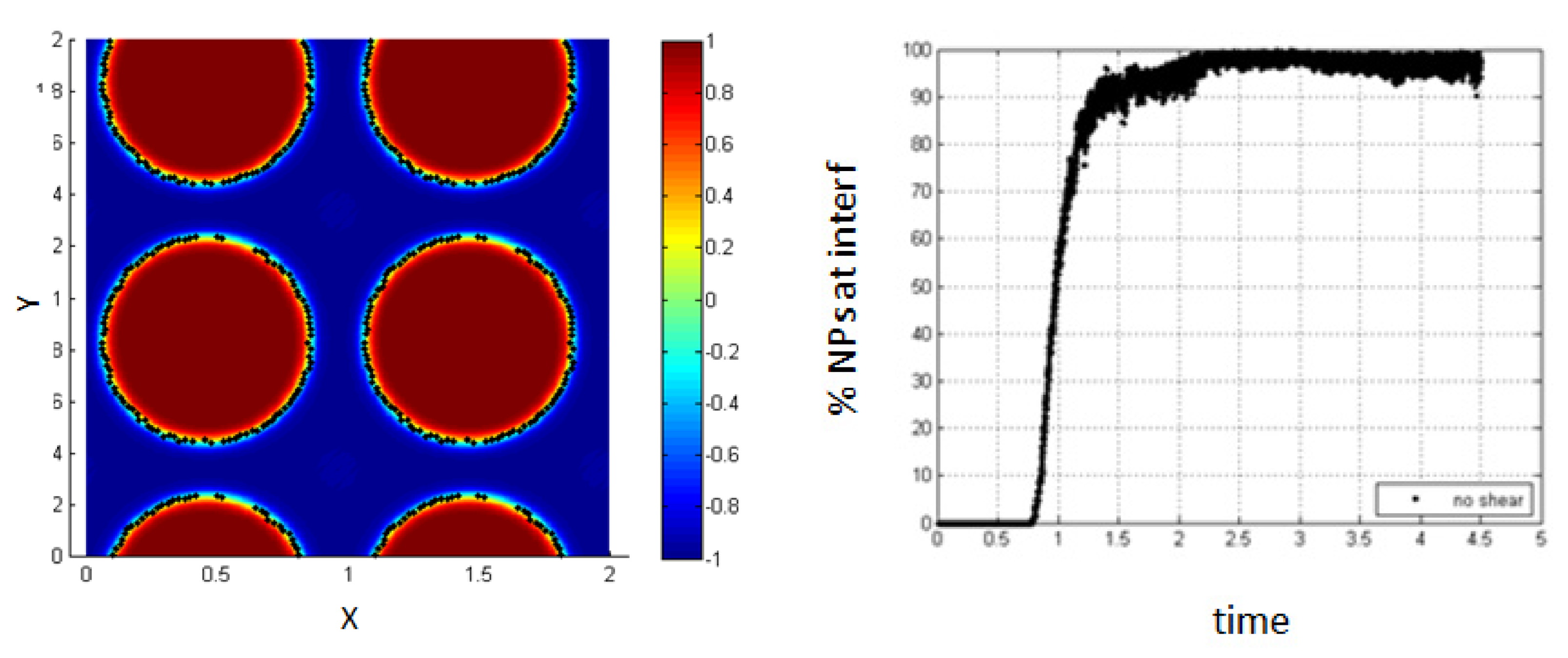
3.1. Fluids Separation and Interface Formation
3.2. Introduction of Nanoparticles after the Separation of the Two Fluids and the Formation of the Interface
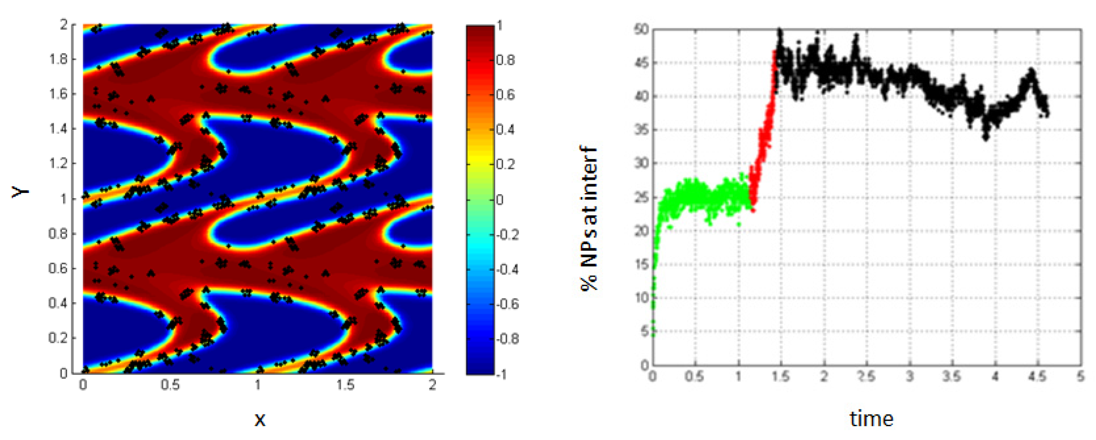
3.2.1. Low Concentration of Nanoparticles
- Neglect particle–particle interactions
- No shear case.
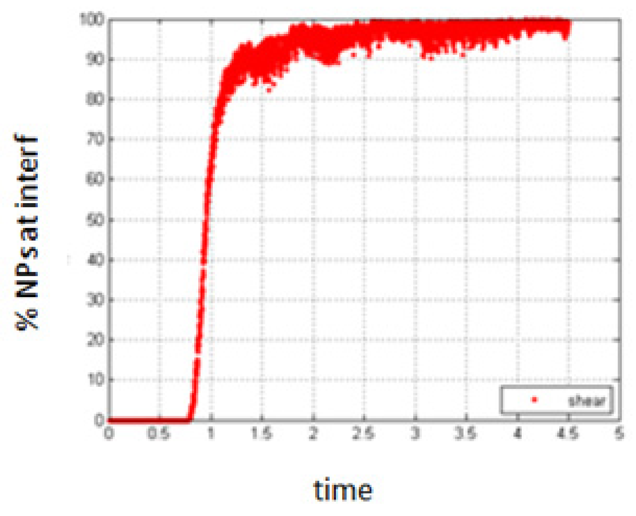
- 2.
- Simulation with shear rate = 0.4; Pe = 0.008, T-shear = 0.3.
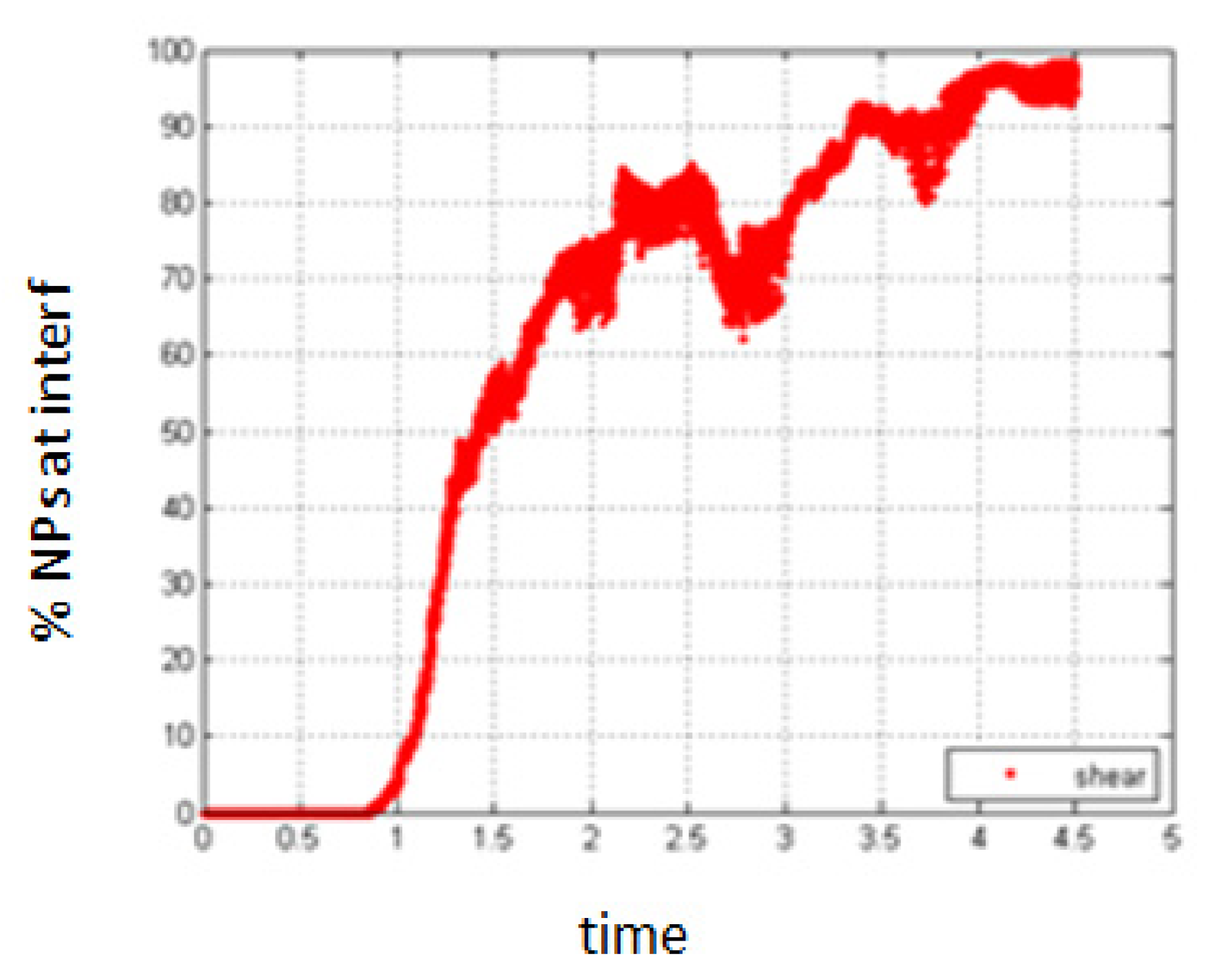
- 3.
- Simulation with shear rate = 7.7; Pe = 0.154, T-shear = 0.3.
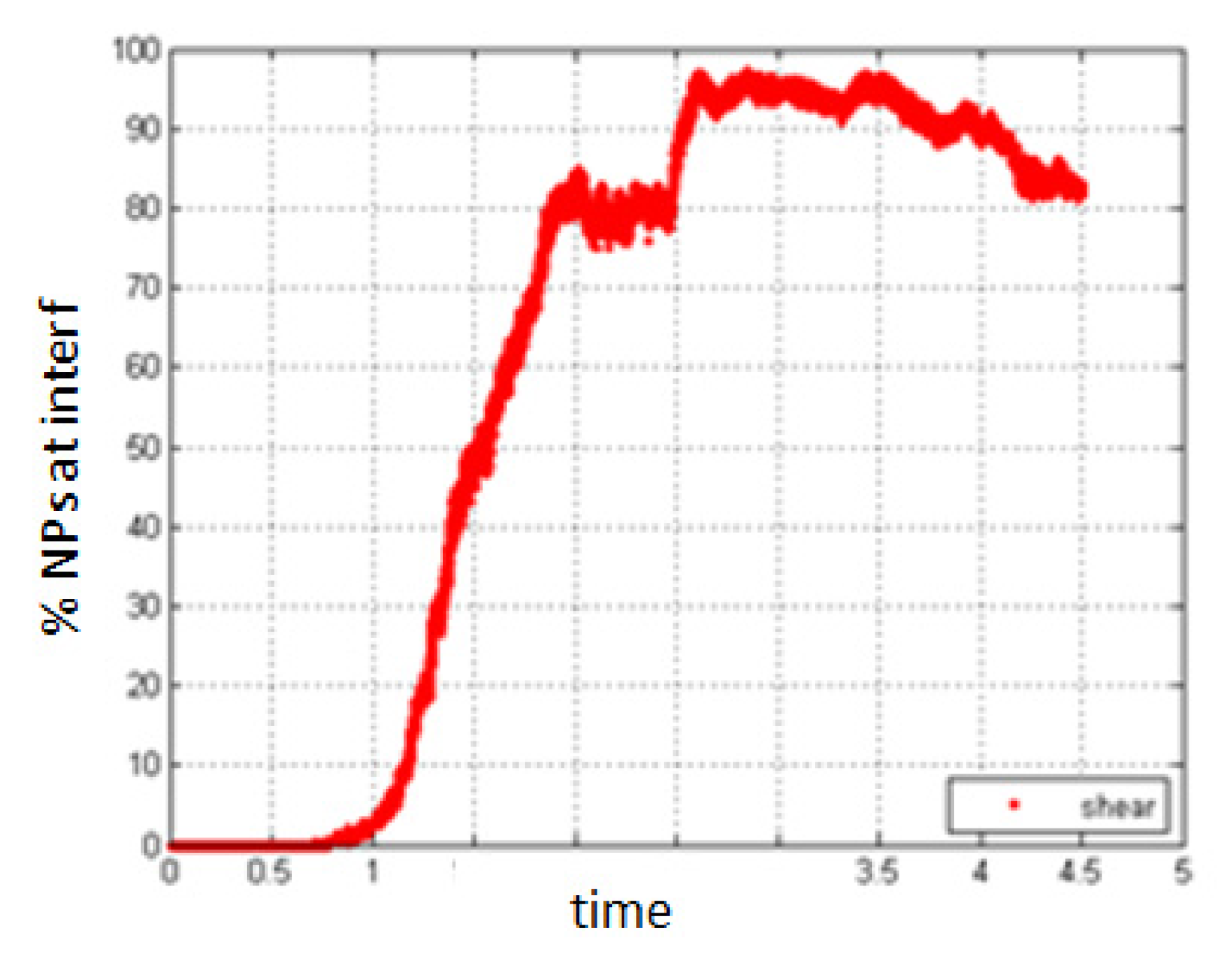
- 4.
- Simulation with shear rate =15.8; Pe = 0.316, T-shear = 0.3.
- Including particle–particle interactions.
- 1.
- No shear case.
- 2.
- Simulation with Pe = 0.008; T-shear = 0.3.
- 3.
- Simulation with shear rate =15.8; Pe = 0.316; T-shear = 0.3.
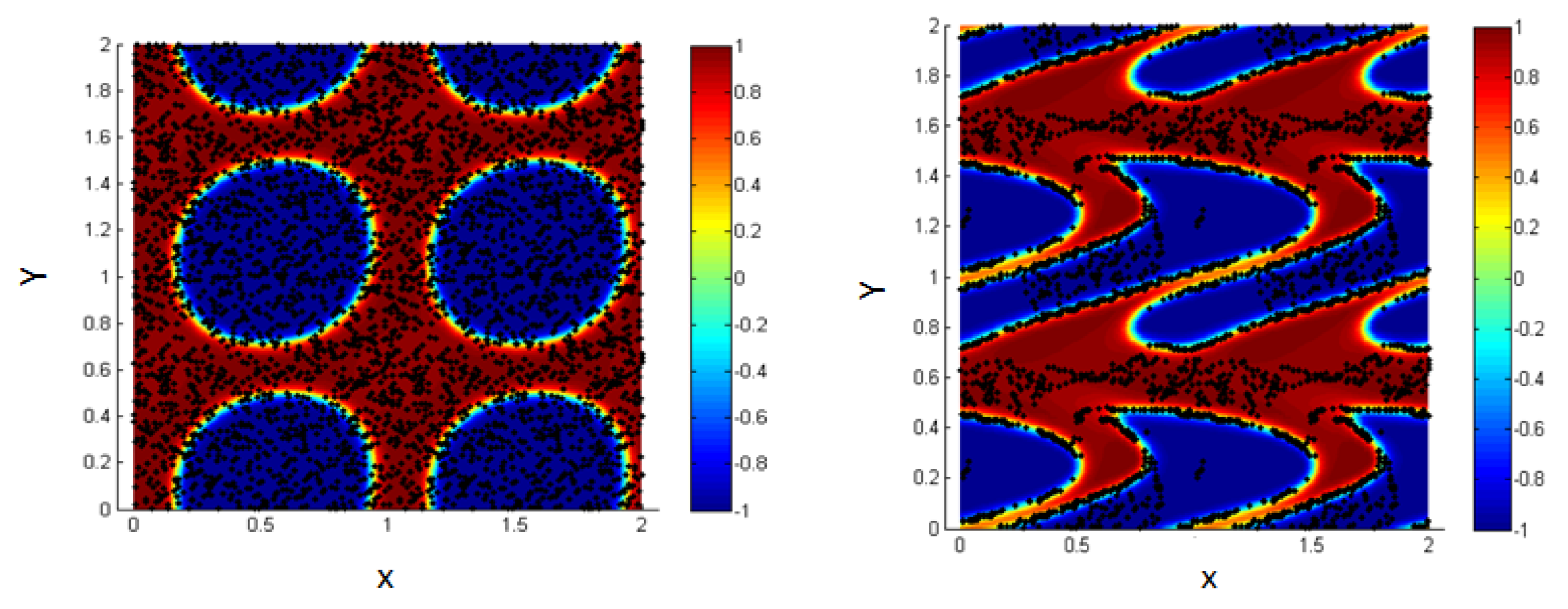
3.2.2. Simulation with High Concentration of NPs
- Simulation of neglecting the L.J.potential.
- Simulation including the L.J. potential.
- 1.
- ,
- 2.
- Simulation with ,
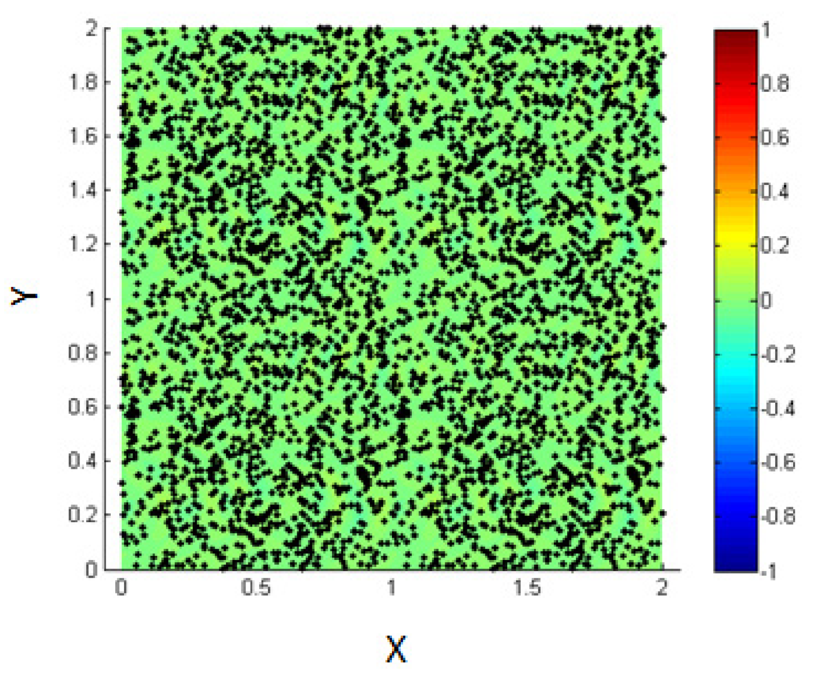
3.3. Introduce the NPs Randomly into the Mixture of the Two Fluids before Phase Separation
- 3.
- Simulation with no shear.
- 4.
- Simulation with shear rate = 0.4; Pe = 0.008
- 5.
- Simulation with shear rate 7.7; Pe = 0.154.
- 6.
- Simulation with shear rate 15.8, Pe = 0.316
4. Conclusions
Author Contributions
Funding
Conflicts of Interest
References
- Bhushan, B. Handbook of Nanotechnology; Springer: Berlin/Heidelberg, Germany, 2006; pp. 17–45. [Google Scholar]
- ShamsiJazeyi, H.; Miller, C.A.; Wong, M.S.; Tour, J.M.; Verduzco, R. Polymer-coated nanoparticles for enhanced oil recovery. J. Appl. Polym. 2014, 131, 40576. [Google Scholar] [CrossRef]
- Cauvin, S.; Clover, P.J.; Bon, S.A.F. Pickering stabilized miniemulsion polymerization: Preparation of clay armored latexes. Macromolecules 2005, 38, 7887–7889. [Google Scholar] [CrossRef]
- Clegg, P.S. Fluid-bicontinuous gels stabilized by interfacial colloids: Low and high molecular weight fluids. J. Phys. Condens. Matter 2008, 20, 113101. [Google Scholar] [CrossRef] [PubMed] [Green Version]
- Whitesides, G.M. The ‘right’ size in Nanobiotechnology. Nat. Biotechnol. 2003, 21, 1161–1165. [Google Scholar] [CrossRef]
- Saleh, N.; Sarbu, T.; Sirk, K.; Lowry, G.V.; Matyjaszewski, K.; Tilton, R.D. Oil-in-water emulsions stabilized by highly charged polyelectrolyte-grafted silica nanoparticles. Langmuir 2005, 21, 9873. [Google Scholar] [CrossRef] [PubMed]
- Horozov, T.S.; Aveyard, R.; Clint, J.H.; Neumann, B. Particle zips: Vertical emulsion films with particle monolayers at their surfaces. Langmuir 2005, 21, 2330. [Google Scholar] [CrossRef]
- Grabinski, C.; Sharma, M.; Maurer, E.; Sulentic, C.; Mohan Sankaran, R.; Hussain, S. The effect of shear flow on nanoparticle agglomeration and deposition in in vitro dynamic flow models. Nanotoxicology 2015, 10, 1–10. [Google Scholar] [CrossRef]
- Arumugam, V.; Redhi, G.; Gengan, R. The application of ionic liquids in nanotechnology. Fundam. Nanoparticles 2018, 371–400. [Google Scholar] [CrossRef]
- Taherkhani, F.; Minofar, B. Static and dynamical properties of colloidal silver nanoparticles in [EMim][PF6] ionic liquid. Ion. Liq. 2019, 129–144. [Google Scholar] [CrossRef]
- Taherkhani, F.; Minofar, B. Effect of Nitrogen Doping on Glass Transition and Electrical Conductivity of [EMIM][PF6] Ionic Liquid Encapsulated in a Zigzag Carbon Nanotube. J. Phys. Chem. C 2017, 121, 15493–15508. [Google Scholar] [CrossRef]
- Kalra, V.; Escobedo, F.; Jooa, Y.L. Effect of shear on nanoparticle dispersion in polymer melts: A coarse-grained molecular dynamics study. J. Chem. Phys. 2010, 132, 024901. [Google Scholar] [CrossRef] [PubMed]
- Kalra, V.; Mendez, S.; Escobedo, F.; Jooj, Y.L. Coarse-grained molecular dynamics simulation on the placement of nanoparticles within symmetric diblock copolymers under shear flow. J. Chem. Phys. 2008, 128, 164909. [Google Scholar] [CrossRef] [Green Version]
- Vo, M.D.; Papavassiliou, D.V. The effects of shear and particle shape on the physical adsorption of polyvinyl pyrrolidone on carbon nanoparticles. Nanotechnology 2016, 27, 325709. [Google Scholar] [CrossRef] [PubMed]
- Kang, T.; Park, C.; Choi, J.S.; Cui, J.H.; Lee, B.J. Effects of shear stress on the cellular distribution of polystyrene nanoparticles in a biomimetic microfluidic system. J. Drug Deliv. Sci. Technol. 2016, 31, 130–136. [Google Scholar] [CrossRef]
- Plattier, J.; Benyahia, L.; Dorget, M.; Niepceron, F.; Tassin, J.F. Viscosity-induced filler localisation in immiscible polymer blends. Polymer 2015, 59, 260–269. [Google Scholar] [CrossRef]
- Becu, L.; Benyahia, L. Strain-Induced Droplet Retraction Memory in a Pickering Emulsion. Langmuir 2009, 25, 6678–6682. [Google Scholar] [CrossRef]
- Daher, A.; Ammar, A.; Hijazi, A. Nanoparticles migration near liquid-liquid interfaces using diffuse interface model. Eng. Comput. 2019, 36, 1036–1054. [Google Scholar] [CrossRef]
- Choi, Y.J.; Djilali, N. Direct numerical simulations of agglomeration of circular colloidal particles in two dimensional shear flow Phys. Fluids 2016, 28, 013304. [Google Scholar] [CrossRef]
- Lowengrub, J.; Truskinovsky, L. Quasi-incompressible Cahn-Hilliard fluids and topological transitions. Proc. R. Soc. A 1998, 454, 2617–2654. [Google Scholar] [CrossRef]
- Cahn, J.W.; Hilliard, J.E. Free energy of a nonuniform system. III. Nucleation in a two-component incompressible fluid. J. Chem. Phys. 1959, 31, 688–699. [Google Scholar] [CrossRef]
- Choi, Y.J.; Anderson, P.D. Cahn–Hilliard modeling of particles suspended in two-phase flows. Int. J. Numer. Methods Fluids 2012, 69, 995–1015. [Google Scholar] [CrossRef]
- Binks, B.P.; Horozov, T.S. (Eds.) University of Hull. Colloidal Particles at Liquid Interfaces; Cambridge University Press: Cambridge, UK, 2006; ISBN 9780511536670. [Google Scholar] [CrossRef]
- Ibarra-Gomez, R.; Marquez, A.; Valle, L.; Rodriguez-Fernandez, O.S. Influence of the Blend Viscosity and Interface Energies on the Preferential Location of CB and Conductivity of BR/EPDM Blends. Rubber Chem. Technol. 2003, 76, 969–978. [Google Scholar] [CrossRef]
- Elias, L.; Fenouillot, F.; Majeste, J.C.; Cassagnau, P. Morphology and rheology of immiscible polymer blends filled with silica nanoparticles. Polymer 2007, 48, 6029e40. [Google Scholar] [CrossRef]
- Elias, L.; Fenouillot, F.; Majeste, J.C.; Alcouffe, P.; Cassagnau, P. Immiscible polymer blends stabilized with nano-silica particles: Rheology and effective interfacial tension. Polymer 2008, 49, 4378–4385. [Google Scholar] [CrossRef]
- Elias, L.; Fenouillot, F.; Majeste, J.C.; Cassagnau, P. Morphology and Rheology of Polymer Blends Filled with Silica Nano Particles . J Polym. Sci.Part B Polym. Phys. 2008, 46, 1976–1983. [Google Scholar]
- Keal, L.; Colosqui, C.E.; Tromp, R.H.; Monteux, C. Colloidal Particle Adsorption at Water-Water Interfaces with Ultralow Interfacial Tension. Phys. Rev. Lett. 2018, 120, 208003. [Google Scholar] [CrossRef] [PubMed] [Green Version]
- Watson, K.J.; Zhu, J.; Nguyen, S.T.; Mirkin, C.A. Hybrid Nanoparticles with Block Copolymer Shell Structures. J. Am. Chem. Soc. 1999, 121, 462. [Google Scholar] [CrossRef]
- Skaff, H.; Ilker, M.F.; Coughlin, E.B.; Emrick, T. Preparation of cadmium selenide-polyolefin composites from functional phosphine oxides and ruthenium-based metathesis. J. Am. Chem. Soc. 2002, 124, 5729–5733. [Google Scholar] [CrossRef]


| Concentration “C” | Liquid 1 | Liquid 2 |
|---|---|---|
| −1 | 100% | 0% |
| 1 | 0% | 100% |
| 0 | 50% | 50% |
Publisher’s Note: MDPI stays neutral with regard to jurisdictional claims in published maps and institutional affiliations. |
© 2021 by the authors. Licensee MDPI, Basel, Switzerland. This article is an open access article distributed under the terms and conditions of the Creative Commons Attribution (CC BY) license (https://creativecommons.org/licenses/by/4.0/).
Share and Cite
Daher, A.; Ammar, A.; Hijazi, A.; Benyahia, L. Effect of Shear Flow on Nanoparticles Migration near Liquid Interfaces. Entropy 2021, 23, 1143. https://doi.org/10.3390/e23091143
Daher A, Ammar A, Hijazi A, Benyahia L. Effect of Shear Flow on Nanoparticles Migration near Liquid Interfaces. Entropy. 2021; 23(9):1143. https://doi.org/10.3390/e23091143
Chicago/Turabian StyleDaher, Ali, Amine Ammar, Abbas Hijazi, and Lazhar Benyahia. 2021. "Effect of Shear Flow on Nanoparticles Migration near Liquid Interfaces" Entropy 23, no. 9: 1143. https://doi.org/10.3390/e23091143
APA StyleDaher, A., Ammar, A., Hijazi, A., & Benyahia, L. (2021). Effect of Shear Flow on Nanoparticles Migration near Liquid Interfaces. Entropy, 23(9), 1143. https://doi.org/10.3390/e23091143