
Modelling and Analysis of the Epidemic Model under Pulse Charging in Wireless Rechargeable Sensor Networks


Abstract
:1. Introduction
2. Epidemic Modeling
2.1. Epidemic Model under Continuous Charging Based on WSNs
2.2. A Pulse Charging Model for SILS
3. Stability of a Malware-Free T-Period Solution
4. Persistence of Malware Transmission
- (a)
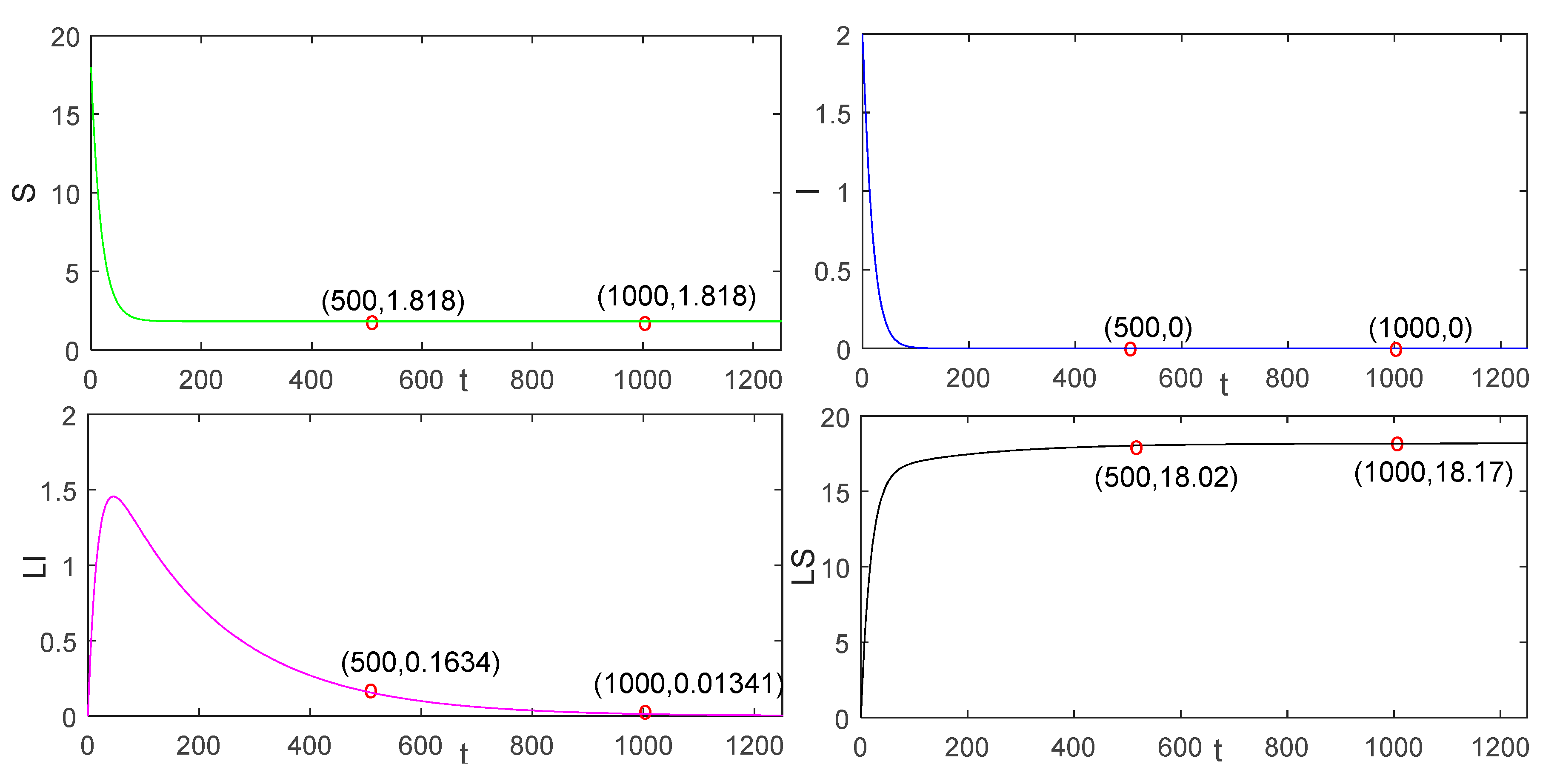
- When the time variable T is large enough, , ;
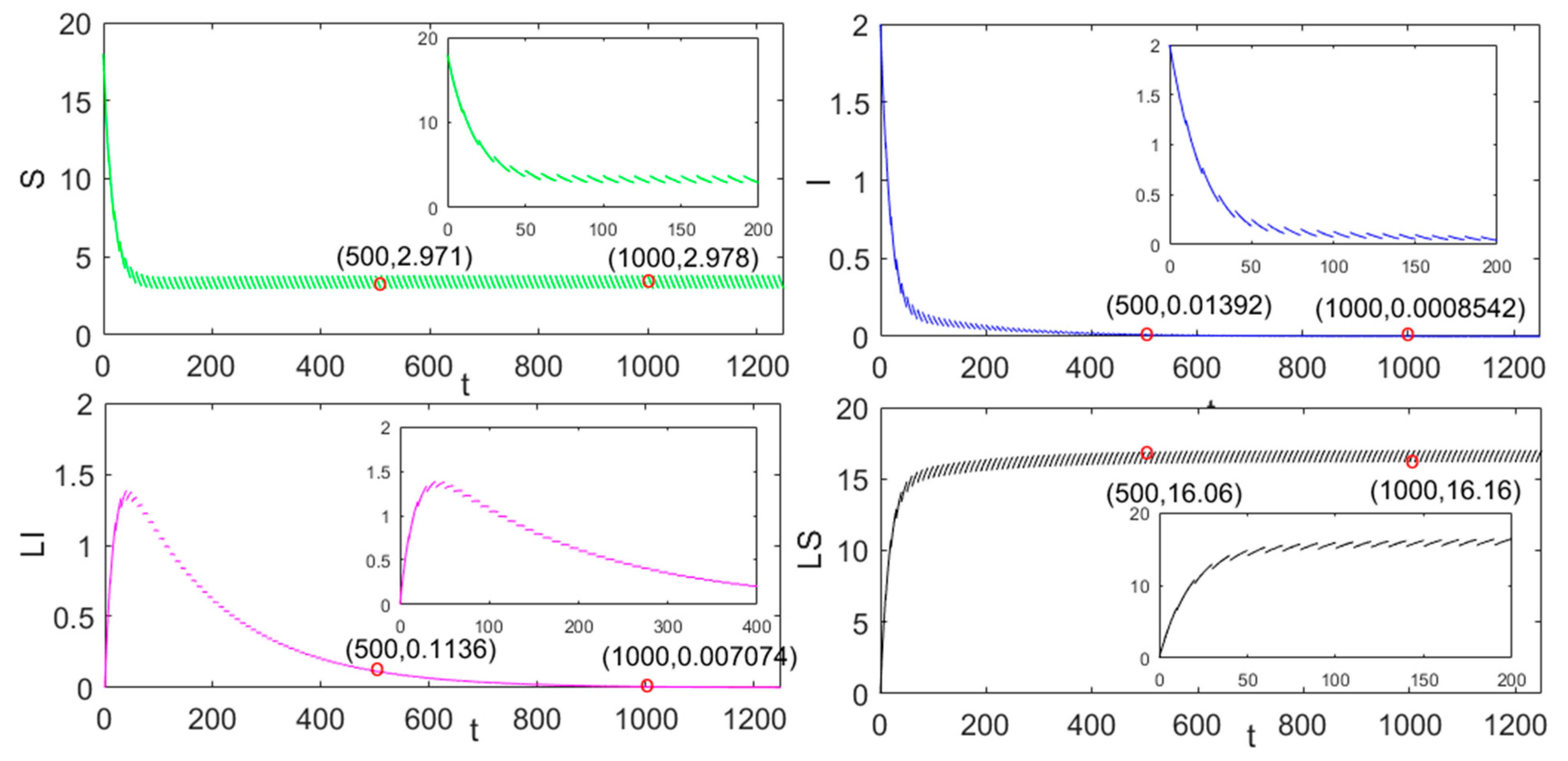
- (b)
- When the time variable T is large enough, and oscillate around .
5. Numerical Simulation
5.1. The Global Stability of the Disease-Free Equilibrium Solution
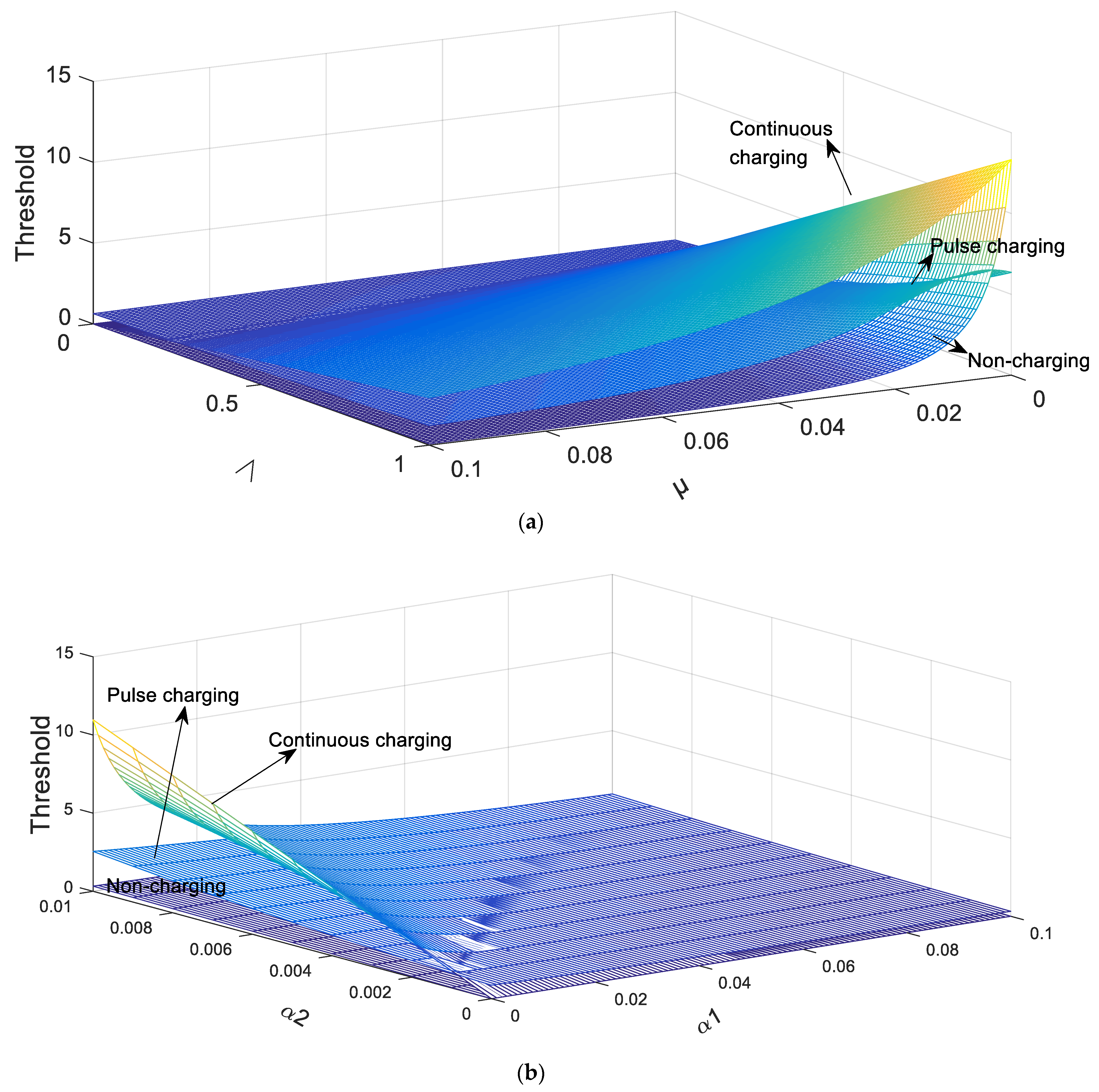
5.2. Relations between the Threshold and Parameters
6. Conclusions and Future Work
Author Contributions
Funding
Institutional Review Board Statement
Informed Consent Statement
Data Availability Statement
Conflicts of Interest
References
- Huang, Y.H.; Zhu, Q.Y. A Differential Game Approach to Decentralized Virus-Resistant Weight Adaptation Policy over Complex Networks. IEEE Trans. Control Netw. Syst. 2020, 7, 944–955. [Google Scholar] [CrossRef] [Green Version]
- Xu, X.T.; Wang, G.C.; Hu, J.T.; Lu, Y.T. Study on Stochastic Differential Game Model in Network Attack and Defense. Secur. Commun. Netw. 2020, 2020, 3417039. [Google Scholar] [CrossRef]
- Wang, H.B.; Feng, L.P. Research on Wireless Sensor Network Security Location Based on Received Signal Strength Indicator Sybil Attack. Discret. Dyn. Nat. Soc. 2020, 2020, 1306084. [Google Scholar] [CrossRef]
- Shanmugavadivel, G.; Gomathy, B.; Ramesh, S.M. An Enhanced Data Security and Task Flow Scheduling in Cloud-enabled Wireless Body Area Network. Wirel. Pers. Commun. 2021. [Google Scholar] [CrossRef]
- Yang, L.; Lu, Y.Z.; Yang, S.M.X.; Guo, T.; Liang, Z.F. A Secure Clustering Protocol with Fuzzy Trust Evaluation and Outlier Detection for Industrial Wireless Sensor Networks. IEEE Trans. Ind. Inform. 2021, 17, 4837–4847. [Google Scholar] [CrossRef]
- Khadr, M.H.; Elgala, H.; Rahaim, M.; Khreishah, A.; Ayyash, M.; Little, T. Machine learning-based security-aware spatial modulation for heterogeneous radio-optical networks. Proc. R. Soc. A-Math. Phys. Eng. Sci. 2021, 477. [Google Scholar] [CrossRef]
- Singh, A.; Nagar, J.; Sharma, S.; Kotiyal, V. A Gaussian process regression approach to predict the k-barrier coverage probability for intrusion detection in wireless sensor networks. Expert Syst. Appl. 2021, 172. [Google Scholar] [CrossRef]
- Singh, D.; Kumar, B.; Singh, S.; Chand, S. A Secure IoT-Based Mutual Authentication for Healthcare Applications in Wireless Sensor Networks Using ECC. Int. J. Healthc. Inf. Syst. Inform. 2021, 16, 21–48. [Google Scholar] [CrossRef]
- Sun, N.; Li, T.; Song, G.F.; Xia, H.R. Network Security Technology of Intelligent Information Terminal Based on Mobile Internet of Things. Mob. Inf. Syst. 2021, 2021, 9. [Google Scholar] [CrossRef]
- Reddy, D.L.; Puttamadappa, C.G.; Suresh, H.N.G. Hybrid optimization algorithm for security aware cluster head selection process to aid hierarchical routing in wireless sensor network. IET Commun. 2021. [Google Scholar] [CrossRef]
- Abidoye, A.P.; Kabaso, B. Lightweight models for detection of denial-of-service attack in wireless sensor networks. IET Netw. 2021. [Google Scholar] [CrossRef]
- Al-Saeed, Y.; Eldaydamony, E.; Atwan, A.; Elmogy, M.; Ouda, O. Efficient Key Agreement Algorithm for Wireless Body Area Networks Using Reusable ECG-Based Features. Electronics 2021, 10, 404. [Google Scholar] [CrossRef]
- Liu, B.; Zhou, W.L.; Gao, L.X.; Zhou, H.B.; Luan, T.H.; Wen, S. Malware Propagations in Wireless Ad Hoc Networks. IEEE Trans. Dependable Secur. Comput. 2018, 15, 1016–1026. [Google Scholar] [CrossRef]
- Wang, X.M.; He, Z.B.; Zhang, L.C. A Pulse Immunization Model for Inhibiting Malware Propagation in Mobile Wireless Sensor Networks. Chin. J. Electron. 2014, 23, 810–815. [Google Scholar]
- Liu, G.Y.; Peng, B.H.; Zhong, X.J. Epidemic Analysis of Wireless Rechargeable Sensor Networks Based on an Attack-Defense Game Model. Sensors 2021, 21, 594. [Google Scholar] [CrossRef]
- Cao, Y.L.; He, Z.B.; Wang, X.M. Optimal Security Strategy for Malware Propagation in Mobile Wireless Sensor Networks. Acta Electron. Sin. 2016, 44. [Google Scholar] [CrossRef]
- Lin, C.; Guo, C.Y.; Dai, H.P.; Wang, L.; Wu, G.W.; Soc, I.C. Near Optimal Charging Scheduling for 3-D Wireless Rechargeable Sensor Networks with Energy Constraints. In Proceedings of the 2019 39th IEEE International Conference on Distributed Computing Systems, Dallas, TX, USA, 7–10 July 2019; pp. 624–633. [Google Scholar]
- Tian, M.; Jiao, W.; Chen, Y. A Joint Energy Replenishment and Data Collection Strategy in Heterogeneous Wireless Rechargeable Sensor Networks. Sensors 2021, 21, 2930. [Google Scholar] [CrossRef]
- Chawra, V.K.; Gupta, G.P. Hybrid meta-heuristic techniques based efficient charging scheduling scheme for multiple Mobile wireless chargers based wireless rechargeable sensor networks (Jan, 10.1007/s12083-020-01052-8, 2021). Peer-to-Peer Netw. Appl. 2021, 14, 1316. [Google Scholar] [CrossRef]
- Tony, T.; Soh, S.; Chin, K.W.; Lazarescu, M. Link Scheduling in Rechargeable Wireless Sensor Networks with Imperfect Battery and Memory Effects. IEEE Access 2021, 9, 17803–17819. [Google Scholar] [CrossRef]
- Liu, G.Y.; Peng, B.H.; Zhong, X.J. A Novel Epidemic Model for Wireless Rechargeable Sensor Network Security. Sensors 2021, 21, 123. [Google Scholar] [CrossRef] [PubMed]
- Lu, X.; Wang, P.; Niyato, D.; Kim, D.I.; Han, Z. Wireless Charging Technologies: Fundamentals, Standards, and Network Applications. IEEE Commun. Surv. Tutor. 2016, 18, 1413–1452. [Google Scholar] [CrossRef] [Green Version]
- Yang, Y.P.; Xiao, Y.N. The effects of population dispersal and pulse vaccination on disease control. Math. Comput. Model. 2010, 52, 1591–1604. [Google Scholar] [CrossRef]
- Berhe, H.W.; Al-arydah, M. Computational modeling of human papillomavirus with impulsive vaccination. Nonlinear Dyn. 2021, 103, 925–946. [Google Scholar] [CrossRef]
- Zhuang, K.C.; Zhang, H.; Zhang, K.; Zhang, H. Analysis of Spreading Dynamics of Virus in Wireless Sensor Networks. Comput. Sci. 2013, 40, 187–191. [Google Scholar]
- Tang, S.S.; Mark, B.L. Analysis of Virus Spread in Wireless Sensor Networks: An Epidemic Model; IEEE: New York, NY, USA, 2009; pp. 86–91. [Google Scholar]


| Authors | Participants | Goal |
|---|---|---|
| Xiaotong Xu et al. [2] | Attack and defense based on evolutionary game theory | Obtain higher security benefits, more suitable for the actual situation of network attack and defense |
| Hongbin Wang et al. [3] | Sensor network node under the attack of Sybil | Accurate detection of Sybil attacks using RSSI |
| G. Shanmugavadivel et al. [4] | Data security in wireless body area networks (WBAN) | Based on AES and efficient task flow scheduling, an enhanced data security model using genetic GA is proposed |
| Liu Yang et al. [5] | Clustering security in industrial wireless sensor networks (IWSNS) | A cluster head selection method based on fuzzy theory is proposed to balance energy saving and safety |
| Monette H. Khadr et al. [6] | Data security in heterogeneous networks | A key selection algorithm for protecting data is proposed. |
| Abhilash Singh et al. [7] | Attack and defense in WSNs | An intrusion prevention method based on Gaussian Process Regression (GPR) model and machine learning is proposed |
| Deepti Singh et al. [8] | Attack and defense in wireless medical sensor networks (WMSNs) | This paper presents an elliptic curve cryptosystem (ECC) based on random prediction model |
| Ning Sun et al. [9] | Security of information transmission in WSNs | The key management and design technology of encryption technology are improved |
| Parameters | Interpretation | Units | Source |
|---|---|---|---|
| The birth rate of nodes | 0.1 | [21] | |
| The mortality rate of nodes | 0.005 | [21] | |
| The rate of transforming both the high-energy nodes and into the low-energy nodes and | 0.05 | [21] | |
| The data transfer coefficient | 0.001 | [21] | |
| The conversion rate of infected nodes become susceptible nodes | 0.01 | [21] | |
| The charging rate of nodes | 0.05 | [21] | |
| The period of pulse charging | 10 | Assumed | |
| The whole number of sensor nodes | 20 | Assumed |
Publisher’s Note: MDPI stays neutral with regard to jurisdictional claims in published maps and institutional affiliations. |
© 2021 by the authors. Licensee MDPI, Basel, Switzerland. This article is an open access article distributed under the terms and conditions of the Creative Commons Attribution (CC BY) license (https://creativecommons.org/licenses/by/4.0/).
Share and Cite
Liu, G.; Huang, Z.; Wu, X.; Liang, Z.; Hong, F.; Su, X. Modelling and Analysis of the Epidemic Model under Pulse Charging in Wireless Rechargeable Sensor Networks. Entropy 2021, 23, 927. https://doi.org/10.3390/e23080927
Liu G, Huang Z, Wu X, Liang Z, Hong F, Su X. Modelling and Analysis of the Epidemic Model under Pulse Charging in Wireless Rechargeable Sensor Networks. Entropy. 2021; 23(8):927. https://doi.org/10.3390/e23080927
Chicago/Turabian StyleLiu, Guiyun, Ziyi Huang, Xilai Wu, Zhongwei Liang, Fenghuo Hong, and Xiaokai Su. 2021. "Modelling and Analysis of the Epidemic Model under Pulse Charging in Wireless Rechargeable Sensor Networks" Entropy 23, no. 8: 927. https://doi.org/10.3390/e23080927
APA StyleLiu, G., Huang, Z., Wu, X., Liang, Z., Hong, F., & Su, X. (2021). Modelling and Analysis of the Epidemic Model under Pulse Charging in Wireless Rechargeable Sensor Networks. Entropy, 23(8), 927. https://doi.org/10.3390/e23080927