
A Factor Analysis Perspective on Linear Regression in the ‘More Predictors than Samples’ Case


Abstract
:1. Introduction
- for Gaussian joint Bayes:where is an input observation, () are the parameters of a GMM, observable is the class index corresponding to , j is a class index, and is the indicator function, which returns 1 if the condition is true and 0 otherwise.
- for expectation–maximization (EM) for the GMM, which optimizes a function concerning a Kullback–Leibler (KL) divergence or the entropy of a random variable—check Appendix A for these details—:E step:M step:where is an input observation, () are the parameters of a GMM, unobservable is the cluster index corresponding to , j is a cluster index, and is the probability that belongs to cluster j.
- linear regression when ,
- semisupervised linear regression when ,
- (semisupervised) linear regression when with missing data.
2. Theoretical Background
2.1. Linear Regression
- Let be a matrix. Then, the Moore–Penrose inverse of A can be defined as , which, algorithmically, is computed via the singular value decomposition of A ([6] Section 2.9). One may notice that the matrix from Equation (3) is just when is invertible. When it is not, the solution is to replace the matrix from Equation (3) with .
- L2 regularization, which results in ridge regression ([2] p. 225). The matrix from Equation (3) is replaced with , with ; the bigger the , the more regularization we add to the model, i.e., move away from overfitting. From this point of view, the first solution using the Moore–Penrose inverse can be interpreted as achieving the asymptotically lowest L2 regularization.
2.2. Factor Analysis
3. Related Work
4. Proposed Models
4.1. The S2.FA Model
4.1.1. The S2.FA Model. S2.FA and S2.UncFA
4.1.2. The S2.FA Model. The Link between LR and S2.UncFA
4.1.3. The S2.FA Model. A New Approach for LR When
4.2. The S3.FA Model
4.3. The MS3.FA Model
5. Experiments
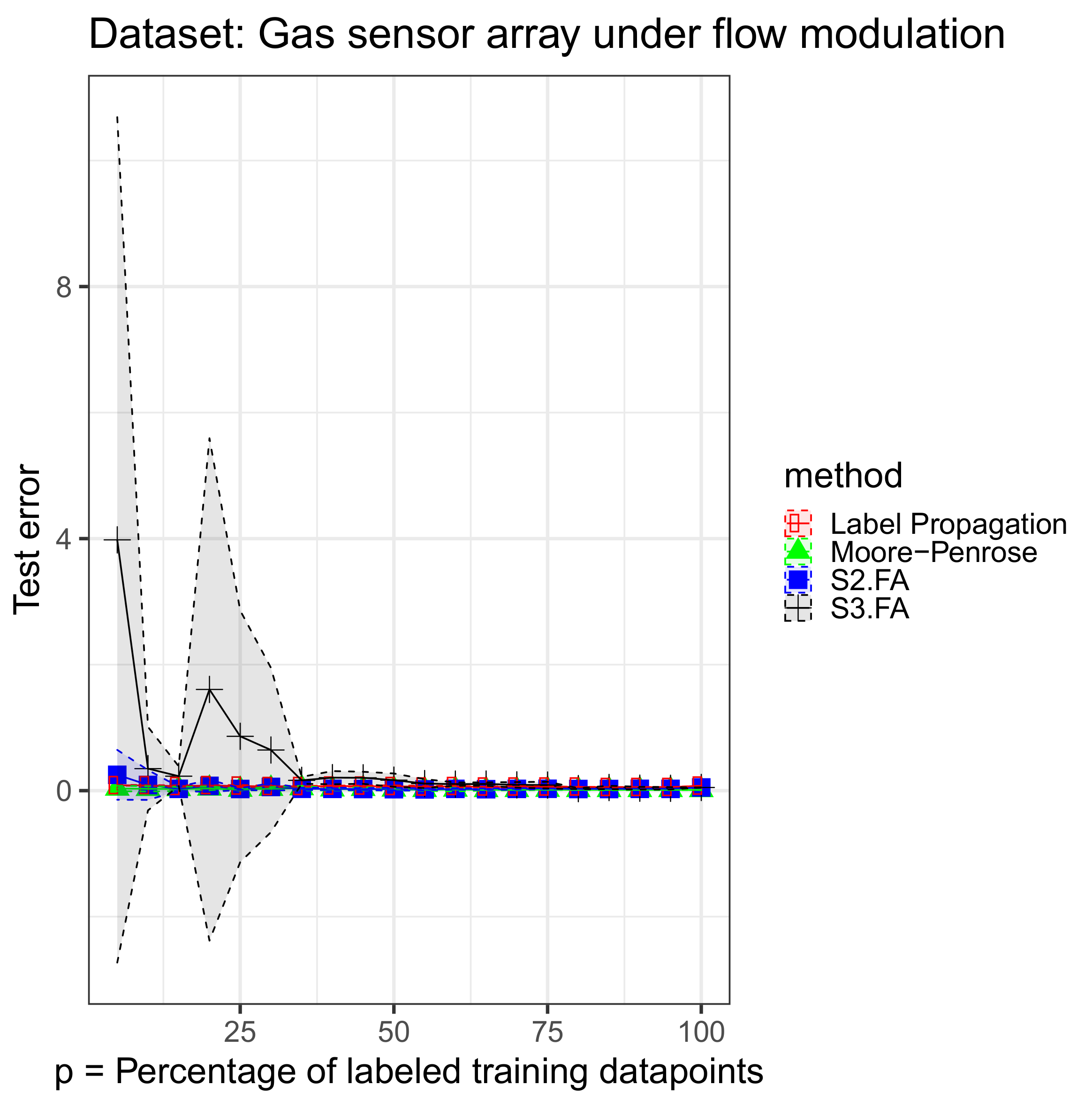
- Gas sensor array under flow modulation data set (http://archive.ics.uci.edu/ml/datasets/Gas+sensor+array+under+flow+modulation; accessed on 31 July 2021) [13]: 58 observations, 432 input attributes;
- atp1d—the airline ticket price; 1D refers to the fact that the target price is in the next day—(https://www.openml.org/d/41475; accessed on 31 July 2021) [14]: 337 observations, 411 input attributes; 370 after preprocessing: see below;
- m5spec—corn measured on a NIR spectrometer: mp5 instrument—(http://www.eigenvector.com/data/Corn; accessed on 31 July 2021): 80 observations, 700 input attributes.
5.1. The S2.FA Model: Experiment
- Moore–Penrose inverse
- ridge regression—L2 regularization
- S2.FA.
5.2. The S3.FA Model: Experiment
5.3. The MS3.FA Model: Experiment
- Mean imputation: for a given attribute (input column), compute its mean ignoring the missing values, then replace the missing data on that attribute with this computed mean
- MS3.FA.
6. Conclusions and Future Work
- of S2.FA with other techniques extending LR to the case,
- of S3.FA with other (semi)supervised regression methods,
- of MS3.FA with another data imputation algorithm.
Author Contributions
Funding
Institutional Review Board Statement
Informed Consent Statement
Data Availability Statement
Acknowledgments
Conflicts of Interest
Abbreviations
| GMM | Gaussian mixture model |
| LR | Linear regression |
| EM | Expectation–maximization |
| KL | Kullback–Leibler |
| FA | Factor analysis |
| PCA | Principal component analysis |
| PPCA | Probabilistic principal component analysis |
| GPLVM | Gaussian process latent variable model |
| MLE | Maximum likelihood estimation |
| UncFA | Unconstrained factor analysis |
| S2.UncFA | Simple-supervised unconstrained factor analysis |
| S2.FA | Simple-supervised factor analysis |
| S2.PPCA | Simple-supervised probabilistic principal component analysis |
| S3.UncFA | Simple-semisupervised unconstrained factor analysis |
| S3.FA | Simple-semisupervised factor analysis |
| S3.PPCA | Simple-semisupervised probabilistic principal component analysis |
| MS3.UncFA | Missing simple-semisupervised unconstrained factor analysis |
| MS3.FA | Missing simple-semisupervised factor analysis |
| MS3.PPCA | Missing simple-semisupervised probabilistic principal component analysis |
| MSE | Mean squared error |
| ELBO | Evidence lower bound |
Appendix A. On the Expectation–Maximization Algorithm
- via (block) coordinate ascentThe resulting meta-algorithm is the EM algorithm.EM is an iterative algorithm and an iteration encompasses two steps:
- E step:for fixed—from the previous iteration.Since , we have:(In this case, we have .)So, we obtained the distribution as a posterior distribution. Although in classic models where conjugate priors are used it is tractable to compute —this type of inference is called analytical inference—, in other models this is not the case and a solution to this shortcoming is represented by approximate/variational inference.
- M step:for fixed—from the E step.Since , we have:So, we obtained a relatively simpler term to maximize. Note that the maximization is further customized using the probabilistic assumptions at hand.
- via gradient ascent: this is the case of Variational Autoencoder [24] which will not be discussed since it is not necessarily relevant to this study.
Appendix B. S2.FA
| Algorithm A1 S2.FA—nonmatrix form. |
|
| Algorithm A2 S2.FA—matrix form. |
|
Appendix C. S3.FA
| Algorithm A3 S3.FA—nonmatrix form. |
|
| Algorithm A4 S3.FA—matrix form. |
|
Appendix D. MS3.FA
| Algorithm A5 MS3.FA—Other functions. |
|
| Algorithm A6 MS3.FA—Train. |
|
| Algorithm A7 MS3.FA—Test and Impute. |
|
References
- Mitchell, T. Generative and Discriminative Classifiers: Naive Bayes and Logistic Regression. (Additional Chapter to Machine Learning; McGraw-Hill: New York, NY, USA, 1997.) Published Online. 2017; Available online: https://bit.ly/39Ueb4o (accessed on 31 July 2021).
- Murphy, K. Machine Learning: A Probabilistic Perspective; MIT Press: Cambridge, MA, USA, 2012. [Google Scholar]
- Ng, A. Machine Learning Course, Lecture Notes, Mixtures of Gaussians and the EM Algorithm. Available online: http://cs229.stanford.edu/notes2020spring/cs229-notes7b.pdf (accessed on 31 July 2021).
- Singh, A. Machine Learning Course, Homework 4, pr 1.1; CMU: Pittsburgh, PA, USA, 2010; p. 528 in Ciortuz, L.; Munteanu, A.; Bădărău, E. Machine Learning Exercise Book (In Romanian); Alexandru Ioan Cuza University of Iași: Iași, Romania, 2019. Available online: https://bit.ly/320ZuIk (accessed on 31 July 2021).
- Ng, A. Machine Learning Course, Lecture Notes, Part X. Available online: http://cs229.stanford.edu/notes2020spring/cs229-notes9.pdf (accessed on 31 July 2021).
- Goodfellow, I.; Bengio, Y.; Courville, A. Deep Learning; MIT Press: Cambridge, MA, USA, 2016; Available online: http://www.deeplearningbook.org (accessed on 31 July 2021).
- Tipping, M.E.; Bishop, C.M. Probabilistic Principal Component Analysis. J. R. Stat. Soc. Ser. (Stat. Methodol.) 1999, 61, 611–622. Available online: https://bit.ly/2PCxoRr (accessed on 31 July 2021). [CrossRef]
- Ciobanu, S. Exploiting a New Probabilistic Model: Simple-Supervised Factor Analysis. Master’s Thesis, Alexandru Ioan Cuza University of Iași, Iași, Romania, 2019. Available online: https://bit.ly/31UsBx6 (accessed on 31 July 2021).
- Ng, A. Machine Learning Course, Lecture Notes, Part XI. Available online: http://cs229.stanford.edu/notes2020spring/cs229-notes10.pdf (accessed on 31 July 2021).
- Lawrence, N.D. Gaussian Process Latent Variable Models for Visualisation of High Dimensional Data. Adv. Neural Inf. Process. Syst. 2004, 329–336. Available online: https://papers.nips.cc/paper/2540-gaussian-process-latent-variable-models-for-visualisation-of-high-dimensional-data.pdf (accessed on 31 July 2021).
- Gao, X.; Wang, X.; Tao, D.; Li, X. Supervised Gaussian Process Latent Variable Model for Dimensionality Reduction. IEEE Trans. Syst. Man, Cybern. Part (Cybern.) 2010, 41, 425–434. Available online: https://ieeexplore.ieee.org/document/5545418 (accessed on 31 July 2021).
- Mitchell, T.; Xing, E.; Singh, A. Machine Learning Course, Midterm Exam, pr. 5.3; CMU: Pittsburgh, PA, USA, 2010; p. 565 Ciortuz, L.; Munteanu, A.; Bădărău, E. Machine Learning Exercise Book (In Romanian); Alexandru Ioan Cuza University of Iași: Iași, Romania, 2019. Available online: https://bit.ly/320ZuIk (accessed on 31 July 2021).
- Ziyatdinov, A.; Fonollosa, J.; Fernández, L.; Gutierrez-Gálvez, A.; Marco, S.; Perera, A. Bioinspired early detection through gas flow modulation in chemo-sensory systems. Sens. Actuators Chem. 2015, 206, 538–547. [Google Scholar] [CrossRef] [Green Version]
- Spyromitros-Xioufis, E.; TSOUMAKAS, G.; WILLIAM, G.; Vlahavas, I. Drawing parallels between multi-label classification and multi-target regression. arXiv 2014, arXiv:1211.6581 v2. [Google Scholar]
- Xiaojin, Z.; Zoubin, G. Learning from Labeled and Unlabeled Data with Label Propagation; Technical Report CMU-CALD-02–107; Carnegie Mellon University: Pittsburgh, PA, USA, 2002. [Google Scholar]
- Wang, J. SSL: Semi-Supervised Learning, R Package Version 0.1; 2016. Available online: https://CRAN.R-project.org/package=SSL (accessed on 31 July 2021).
- Oliver, A.; Odena, A.; Raffel, C.; Cubuk, E.D.; Goodfellow, I.J. Realistic evaluation of deep semi-supervised learning algorithms. arXiv 2018, arXiv:1804.09170. [Google Scholar]
- van Buuren, S.; Groothuis-Oudshoorn, K. Mice: Multivariate Imputation by Chained Equations in R. J. Stat. Softw. 2011, 45, 1–67. Available online: https://www.jstatsoft.org/v45/i03/ (accessed on 31 July 2021). [CrossRef] [Green Version]
- Honaker, J.; King, G.; Blackwell, M. Amelia II: A Program for Missing Data. J. Stat. Softw. 2011, 45, 1–47. Available online: http://www.jstatsoft.org/v45/i07/ (accessed on 31 July 2021). [CrossRef]
- Ghahramani, Z.; Hinton, G.E. The EM Algorithm for Mixtures of Factor Analyzers; Technical Report, CRG-TR-96-1; University of Toronto: Toronto, ON, Canada, 1996; Available online: http://mlg.eng.cam.ac.uk/zoubin/papers/tr-96-1.pdf (accessed on 31 July 2021).
- Bishop, C.M. Pattern Recognition and Machine Learning; Springer Science + Business Media: Berlin, Germany, 2006. [Google Scholar]
- Zaharia, M.; Xin, R.S.; Wendell, P.; Das, T.; Armbrust, M.; Dave, A.; Meng, X.; Rosen, J.; Venkataraman, S.; Franklin, M.J.; et al. Apache Spark: A Unified Engine for Big Data Processing. Commun. ACM 2016, 59, 56–65. [Google Scholar] [CrossRef]
- Dempster, A.P.; Laird, N.M.; Rubin, D.B. Maximum likelihood from incomplete data via the EM algorithm. J. R. Stat. Soc. Ser. (Methodol.) 1977, 39, 1–22. [Google Scholar]
- Kingma, D.P.; Welling, M. Auto-encoding variational bayes. arXiv 2013, arXiv:1312.6114. [Google Scholar]


| Data Set/Method | Moore–Penrose | Ridge Regression | S2.FA |
|---|---|---|---|
| Gas sensor array under flow modulation | 0.0251 ± 0.0254 | 0.0062 ± 0.007 | 0.0452 ± 0.0208 |
| atp1d | 94,627.7239 ± 80,183.0076 | 27,770.9253 ± 42,887.5216 | 4724.2957 ± 1616.3341 |
| m5spec | 0.00004 ± 0.00001 | 0.02676 ± 0.01372 | 0.37344 ± 0.25025 |
| Data Set | Method | |||
|---|---|---|---|---|
| Gas sensor array under flow modulation | Moore–Penrose | 0.034 ± 0.0437 | 0.0292 ± 0.0421 | 0.0267 ± 0.0326 |
| S2.FA | 0.2511 ± 0.3953 | 0.0899 ± 0.2367 | 0.0285 ± 0.0333 | |
| S3.FA | 3.9799 ± 6.7087 | 0.349 ± 0.6626 | 0.2294 ± 0.1561 | |
| Label Propagation | 0.0853 ± 0.0073 | 0.0825 ± 0.0051 | 0.0708 ± 0.013 | |
| atp1d | Moore–Penrose | 3763.2939 ± 749.0966 | 3079.5042 ± 1842.7676 | 3428.7567 ± 1722.6437 |
| S2.FA | 2706.9906 ± 477.3245 | 2339.3504 ± 324.8581 | 2279.0802 ± 99.5443 | |
| S3.FA | 3771.605 ± 1563.6543 | 2972.1137 ± 639.6724 | 2633.0816 ± 274.7409 | |
| Label Propagation | 110,820.3235 ± 0 | 110,820.3235 ± 0 | 110,820.3235 ± 0 | |
| m5spec | Moore–Penrose | 0.4602 ± 0.354 | 0.3609 ± 0.7631 | 0.0187 ± 0.0221 |
| S2.FA | 0.7003 ± 0.3834 | 0.4269 ± 0.5441 | 0.4999 ± 0.5172 | |
| S3.FA | 0.8133 ± 0.6366 | 1.653 ± 3.9497 | 0.5118 ± 0.5503 | |
| Label Propagation | 0.2175 ± 0.0707 | 0.1939 ± 0.0706 | 0.2343 ± 0.0624 | |
| Data Set | Method | |||
| Gas sensor array under flow modulation | Moore–Penrose | 0.0313 ± 0.0259 | 0.0192 ± 0.0145 | 0.0132 ± 0.0075 |
| S2.FA | 0.0588 ± 0.0576 | 0.0233 ± 0.0224 | 0.0279 ± 0.0116 | |
| S3.FA | 0.645 ± 1.3044 | 0.1666 ± 0.1059 | 0.0912 ± 0.0443 | |
| Label Propagation | 0.0668 ± 0.0086 | 0.0675 ± 0.018 | 0.0605 ± 0.0122 | |
| atp1d | Moore–Penrose | 6401.7587 ± 3602.9182 | 7907.484 ± 4449.2312 | 36,041.874 ± 21,300.704 |
| S2.FA | 2444.9001 ± 404.2393 | 2439.162 ± 108.3605 | 2399.7948 ± 160.1038 | |
| S3.FA | 2760.6602 ± 391.9217 | 2659.6472 ± 112.9795 | 2521.9861 ± 222.3765 | |
| Label Propagation | 110,820.3235 ± 0 | 110,820.3235 ± 0 | 110,820.3235 ± 0 | |
| m5spec | Moore–Penrose | 0.00057 ± 0.00085 | 0.00009 ± 0.00008 | 0.00009 ± 0.00004 |
| S2.FA | 0.37449 ± 0.12508 | 0.35796 ± 0.07275 | 0.3995 ± 0.03164 | |
| S3.FA | 0.37865 ± 0.12808 | 0.36181 ± 0.07463 | 0.40419 ± 0.03415 | |
| Label Propagation | 0.19391 ± 0.02754 | 0.17424 ± 0.00857 | 0.17752 ± 0.01545 |
| Data Set | Method | |||
|---|---|---|---|---|
| Gas sensor array under flow modulation | Mean | 0.0108 ± 0.0022 | 0.0241 ± 0.0027 | 0.0359 ± 0.0011 |
| MS3.FA | 0.00603 ± 0.00029 | 0.01176 ± 0.00081 | 0.01747 ± 0.00094 | |
| atp1d | Mean | 3239.9757 ± 68.2511 | 6831.0884 ± 105.6119 | 10,077.1798 ± 117.4693 |
| MS3.FA | 1807.7748 ± 105.03 | 3697.1146 ± 124.2197 | 5276.899 ± 104.6252 | |
| m5spec | Mean | 0.00013 ± 0.00001 | 0.00026 ± 0 | 0.00039 ± 0.00001 |
| MS3.FA | 0.14835 ± 0.000002 | 0.148433 ± 0.000002 | 0.148518 ± 0.000002 | |
| Data Set | Method | |||
| Gas sensor array under flow modulation | Mean | 0.0494 ± 0.0042 | 0.0597 ± 0.0015 | 0.0731 ± 0.0012 |
| MS3.FA | 0.02372 ± 0.00159 | 0.0299 ± 0.00047 | 0.0364 ± 0.0011 | |
| atp1d | Mean | 13,423.3625 ± 252.7735 | 16,899.3166 ± 223.6971 | 20,156.2493 ± 62.1299 |
| MS3.FA | 7071.6793 ± 143.3232 | 8921.5319 ± 165.5759 | 10,558.5723 ± 53.1182 | |
| m5spec | Mean | 0.000521 ± 0.000005 | 0.000658 ± 0.000008 | 0.00080 ± 0.000005 |
| MS3.FA | 0.1486 ± 0.00001 | 0.14869 ± 0.00001 | 0.148781 ± 0.000001 |
Publisher’s Note: MDPI stays neutral with regard to jurisdictional claims in published maps and institutional affiliations. |
© 2021 by the authors. Licensee MDPI, Basel, Switzerland. This article is an open access article distributed under the terms and conditions of the Creative Commons Attribution (CC BY) license (https://creativecommons.org/licenses/by/4.0/).
Share and Cite
Ciobanu, S.; Ciortuz, L. A Factor Analysis Perspective on Linear Regression in the ‘More Predictors than Samples’ Case. Entropy 2021, 23, 1012. https://doi.org/10.3390/e23081012
Ciobanu S, Ciortuz L. A Factor Analysis Perspective on Linear Regression in the ‘More Predictors than Samples’ Case. Entropy. 2021; 23(8):1012. https://doi.org/10.3390/e23081012
Chicago/Turabian StyleCiobanu, Sebastian, and Liviu Ciortuz. 2021. "A Factor Analysis Perspective on Linear Regression in the ‘More Predictors than Samples’ Case" Entropy 23, no. 8: 1012. https://doi.org/10.3390/e23081012
APA StyleCiobanu, S., & Ciortuz, L. (2021). A Factor Analysis Perspective on Linear Regression in the ‘More Predictors than Samples’ Case. Entropy, 23(8), 1012. https://doi.org/10.3390/e23081012