Variational Message Passing and Local Constraint Manipulation in Factor Graphs

Abstract

Accurate evaluation of Bayesian model evidence for a given data set is a fundamental problem in model development. Since evidence evaluations are usually intractable, in practice variational free energy (VFE) minimization provides an attractive alternative, as the VFE is an upper bound on negative model log-evidence (NLE). In order to improve tractability of the VFE, it is common to manipulate the constraints in the search space for the posterior distribution of the latent variables. Unfortunately, constraint manipulation may also lead to a less accurate estimate of the NLE. Thus, constraint manipulation implies an engineering trade-off between tractability and accuracy of model evidence estimation. In this paper, we develop a unifying account of constraint manipulation for variational inference in models that can be represented by a (Forney-style) factor graph, for which we identify the Bethe Free Energy as an approximation to the VFE. We derive well-known message passing algorithms from first principles, as the result of minimizing the constrained Bethe Free Energy (BFE). The proposed method supports evaluation of the BFE in factor graphs for model scoring and development of new message passing-based inference algorithms that potentially improve evidence estimation accuracy.

1. Introduction

Building models from data is at the core of both science and engineering applications. The search for good models requires a performance measure that scores how well a particular model m captures the hidden patterns in a data set D. In a Bayesian framework, that measure is the Bayesian evidence $p\left(D\right|m)$, i.e., the probability that model m would generate D if we were to draw data from m. The art of modeling is then the iterative process of proposing new model specifications, evaluating the evidence for each model and retaining the model with the most evidence [1].

Unfortunately, Bayesian evidence is intractable for most interesting models. A popular solution to evidence evaluation is provided by variational inference, which describes the process of Bayesian evidence evaluation as a (free energy) minimization process, since the variational free energy (VFE) is a tractable upper bound on Bayesian (negative log-)evidence [2]. In practice, the model development process then consists of proposing various candidate models, minimizing VFE for each model and selecting the model with the lowest minimized VFE.

The difference between VFE and negative log-evidence (NLE) is equal to the Kullback–Leibler divergence (KLD) [3] from the (perfect) Bayesian posterior distribution to the variational distribution for the latent variables in the model. The KLD can be interpreted as the cost of conducting variational rather than Bayesian inference. Perfect (Bayesian) inference would lead to zero inference costs (KLD $=0$), and the KLD increases as the variational posterior diverges further from the Bayesian posterior. As a result, model development in a variational inference context is a balancing act, where we search for models that have both large amounts of evidence for the data and small inference costs (small KLD). In other words, in a variational inference context, the researcher has two knobs to tune models. The first knob alters the model specification, which affects model evidence. The second knob relates to constraining the search space for the variational posterior, which may affect the inference costs.

In this paper, we are concerned with developing algorithms for tuning the second knob. How do we constrain the range of variational posteriors so as to make variational inferences both tractable and accurate (resulting in low KLD)? We present our framework in the context of a (Forney-style) factor graph representation of the model [4,5]. In that context, variational inference can be understood as an automatable and efficient message passing-based inference procedure [6,7,8].

Traditional constraints include mean-field [6] and Bethe approximations [9,10]. However, more recently it has become clear how alternative local constraints, such as posterior factorization [11], expectation and chance constraints [12,13], and local Laplace approximation [14], may impact both tractability and inference accuracy, and thereby potentially lead to lower VFE. The main contribution of the current work lies in unifying the various ideas on local posterior constraints into a principled method for deriving variational message passing-based inference algorithms. The proposed method derives existing message passing algorithms, but also supports the development of new message passing variants.

Section 2 reviews Forney-style Factor Graphs (FFGs) and variational inference by minimizing the Bethe Free Energy (BFE). This review is continued in Section 3, where we discuss BFE optimization from a Lagrangian optimization viewpoint. In Appendix A, we include an example to illustrate that the Bayes rule can be derived from Lagrangian optimization with data constraints. Our main contribution lies in Section 4, which provides a rigorous treatment of the effects of imposing local constraints on the BFE and the resulting message update rules. We build upon several previous works that describe how manipulation of (local) constraints and variational objectives can be employed to improve variational approximations in the context of message passing. For example, ref. [12] shows how inference algorithms can be unified in terms of hybrid message passing by Lagrangian constraint manipulation. We extend this view by bringing form (Section 4.2) and factorization constraints (Section 4.1) into a constrained optimization framework. In [15], a high-level recipe for generating message passing algorithms from divergence measures is described. We apply their general recipe in the current work, where we adhere to the view on local stationary points for region-based approximations on general graphs [16]. In Appendix B, we also show that locally stationary solutions are also the global stationary solutions. In Section 5, we develop an algorithm for VFE evaluation in an FFG. In previous work, ref. [17] describes a factor softening approach to evaluate the VFE for models with deterministic factors. We extend this work in Section 5, and show how to avoid factor softening for both free energy evaluation and inference of posteriors. We show an example of how to compute VFE for a deterministic node in Appendix C. A more detailed comparison to related work is given in Section 7.

In the literature, proofs and descriptions of message passing-based inference algorithms are scattered across multiple papers and varying graphical representations, including Bayesian networks [6,18], Markov random fields [16], bi-partite (Tanner) factor graphs [12,17,19] and Forney-style factor graphs (FFGs) [5,11]. In Appendix D, we provide first-principle proofs for a large collection of familiar message passing algorithms in the context of Forney-style factor graphs, which is the preferred framework in the information and communication theory communities [4,20].

2. Factor Graphs and the Bethe Free Energy

2.1. Terminated Forney-Style Factor Graphs

A Forney-style factor graph (FFG) is an undirected graph $\mathcal{G}=(\mathcal{V},\mathcal{E})$ with nodes $\mathcal{V}$ and edges $\mathcal{E}\subseteq \mathcal{V}\times \mathcal{V}$. We denote the neighboring edges of a node $a\in \mathcal{V}$ by $\mathcal{E}\left(a\right)$. Vice versa, for an edge $i\in \mathcal{E}$, the notation $\mathcal{V}\left(i\right)$ collects all neighboring nodes. As a notational convention, we index nodes by $a,b,c$ and edges by $i,j,k$, unless stated otherwise. We will mainly use a and i as summation indices and use the other indices to refer to a node or edge of interest.

In this paper, we will frequently refer to the notion of a subgraph. We define an edge-induced subgraph by $\mathcal{G}\left(i\right)=\left(\mathcal{V}\right(i),i)$, and a node-induced subgraph by $\mathcal{G}\left(a\right)=(a,\mathcal{E}(a\left)\right)$. Furthermore, we denote a local subgraph by $\mathcal{G}(a,i)=\left(\mathcal{V}\right(i),\mathcal{E}(a\left)\right)$, which collects all local nodes and edges around i and a, respectively.

An FFG can be used to represent a factorized function,

$$\begin{array}{c}\hfill f\left(\mathit{s}\right)=\prod _{a\in \mathcal{V}}{f}_a\left({\mathit{s}}_a\right),\end{array}$$

(1)

where ${\mathit{s}}_a$ collects the argument variables of factor $f_a$. We assumed that all the factors are positive. In an FFG, a node $a\in \mathcal{V}$ corresponds to a factor $f_a$, and the neighboring edges $\mathcal{E}\left(a\right)$ correspond to the variables ${\mathit{s}}_a$ that are the arguments of $f_a$.

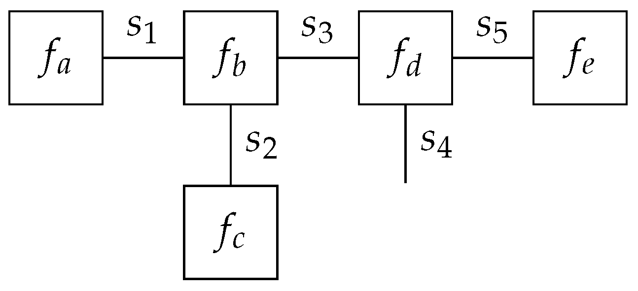
As an example model, the following factorization (2), the corresponding FFG of which is shown in Figure 1.

$$\begin{array}{c}\hfill f(s_1,\cdots ,s_5)=f_a\left(s_1\right)f_b(s_1,s_2,s_3)f_c\left(s_2\right)f_d(s_3,s_4,s_5)f_e\left(s_5\right).\end{array}$$

(2)

The FFG of Figure 1 consists of five nodes $\mathcal{V}=\{a,\dots ,e\}$, as annotated by their corresponding factor functions, and five edges $\mathcal{E}=\left\{\right(a,b),\dots ,(d,e\left)\right\}$ as annotated by their corresponding variables. An edge that connects to only one node (e.g., the edge for $s_4$) is called a half-edge. In this example, the neighborhood $\mathcal{E}\left(b\right)=\left\{\right(a,b),(b,c),(b,d\left)\right\}$ and $\mathcal{V}\left(\right(b,c\left)\right)=\{b,c\}$.

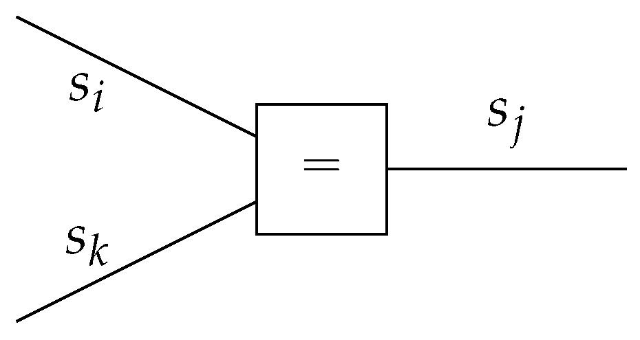
In the FFG representation, a node can be connected to an arbitrary number of edges, while an edge can only be connected to at most two nodes. Therefore, FFGs often contain “equality nodes” that constrain connected edges to carry identical beliefs, with the implication that these beliefs can be made available to more than two factors. An equality node has the factor function

$$\begin{array}{cc}\hfill f_a(s_i,s_j,s_k)& =\delta (s_j-s_i)\delta (s_j-s_k),\hfill \end{array}$$

(3)

for which the node-induced subgraph $\mathcal{G}\left(a\right)$ is drawn in Figure 2.

If every edge in the FFG has exactly two connected nodes (including equality nodes), then we designate the graph as a terminated FFG (TFFG). Since multiplication of a function $f\left(\mathit{s}\right)$ by 1 does not alter the function, any FFG can be terminated by connecting any half-edge i to a node a that represents the unity factor $f_a\left(s_i\right)=1$.

In Section 4.2 we discuss form constraints on posterior distributions. If such a constraint takes on a Dirac-delta functional form, then we visualize the constraint on the FFG by a small circle in the middle of the edge. For example, the small shaded circle in Figure 11 indicates that the variable has been observed. In Section 4.3.2 we consider form constraints in the context of optimization, in which case the circle annotation will be left open (see, e.g., Figure 14).

2.2. Variational Free Energy

Given a model $f\left(\mathit{s}\right)$ and a (normalized) probability distribution $q\left(\mathit{s}\right)$, we can define a Variational Free Energy (VFE) functional as

$$F[q,f]\triangleq \int q\left(\mathit{s}\right)log\frac{q\left(\mathit{s}\right)}{f\left(\mathit{s}\right)}d\mathit{s}.$$

(4)

Variational inference is concerned with finding solutions to the minimization problem

$$\begin{array}{c}\hfill q^{*}\left(\mathit{s}\right)=arg\underset{q\in \mathcal{Q}}{min}F[q,f],\end{array}$$

(5)

where $\mathcal{Q}$ imposes some constraints on q.

If q is unconstrained, then the optimal solution is obtained for $q^{*}\left(\mathit{s}\right)=p\left(\mathit{s}\right)$, with $p\left(\mathit{s}\right)=\frac{1}{Z}f\left(\mathit{s}\right)$ being the exact posterior, and $Z=\int f\left(\mathit{s}\right)d\mathit{s}$ a normalizing constant that is commonly referred to as the evidence. The minimum value of the free energy then follows as the negative log-evidence (NLE),

$$\begin{array}{c}\hfill F[q^{*},f]=-logZ,\end{array}$$

which is also known as the surprisal. The NLE can be interpreted as a measure of model performance, where low NLE is preferred.

As an unconstrained search space for q grows exponentially with the number of variables, the optimization of (5) quickly becomes intractable beyond the most basic models. Therefore, constraints and approximations to the variational free energy (4) are often utilized. As a result, the constrained variational free energy with $q^{*}\in \mathcal{Q}$ bounds the NLE by

$$\begin{array}{c}\hfill F[q^{*},f]=-logZ+\int q^{*}\left(\mathit{s}\right)log\frac{q^{*}\left(\mathit{s}\right)}{p\left(\mathit{s}\right)}d\mathit{s},\end{array}$$

(6)

where the latter term expresses the divergence from the (intractable) exact solution to the optimal variational belief.

In practice, the functional form of $q\left(\mathit{s}\right)=q(\mathit{s};\mathit{\theta })$ is often parameterized, such that gradients of F can be derived w.r.t. the parameters $\mathit{\theta }$. This effectively converts the variational optimization of $F[q,f]$ to a parametric optimization of $F\left(\mathit{\theta }\right)$ as a function of $\mathit{\theta }$. This problem can then be solved by a (stochastic) gradient descent procedure [21,22].

In the context of variational calculus, while form constraints may lead to interesting properties (see Section 4.2), they are generally not required. Interestingly, in a variational optimization context, the functional form of q is often not an assumption, but rather a result of optimization (see Section 4.3.1). An example of variational inference is provided in Appendix A.

2.3. Bethe Free Energy

The Bethe approximation enjoys a unique place in the landscape of $\mathcal{Q}$, because the Bethe free energy (BFE) defines the fundamental objective of the celebrated belief propagation (BP) algorithm [17,23]. The origin of the Bethe approximation is rooted in tree-like approximations to subgraphs (possibly containing cycles) by enforcing local consistency conditions on the beliefs associated with edges and nodes [24].

Given a TFFG $\mathcal{G}=(\mathcal{V},\mathcal{E})$ for a factorized function $f\left(\mathit{s}\right)={\prod }_{a\in \mathcal{V}}{f}_a\left({\mathit{s}}_a\right)$ (1), the Bethe free energy (BFE) is defined as [25]:

$$\begin{array}{cc}\hfill F[q,f]& \triangleq \sum _{a\in \mathcal{V}}\underset{F[q_a,f_a]}{\underbrace{\int q_a\left({\mathit{s}}_a\right)log\frac{q_a\left({\mathit{s}}_a\right)}{f_a\left({\mathit{s}}_a\right)}d{\mathit{s}}_a}}+\sum _{i\in \mathcal{E}}\underset{H\left[q_i\right]}{\underbrace{\int q_i\left(s_i\right)log\frac{1}{q_i\left(s_i\right)}d{s}_i}}\hfill \end{array}$$

(7)

such that the factorized beliefs

$$\begin{array}{cc}\hfill q\left(\mathit{s}\right)& =\prod _{a\in \mathcal{V}}{q}_a\left({\mathit{s}}_a\right)\prod _{i\in \mathcal{E}}{q}_i{\left(s_i\right)}^{-1}\hfill \end{array}$$

(8)

satisfy the following constraints:

$$\begin{array}{cc}\hfill \int q_a\left({\mathit{s}}_a\right)d{\mathit{s}}_a& =1,\mathrm{for}\mathrm{all}a\in \mathcal{V}\hfill \end{array}$$

(9a)

$$\begin{array}{cc}\hfill \int q_a\left({\mathit{s}}_a\right)d{\mathit{s}}_{a\setminus i}& =q_i\left(s_i\right),\mathrm{for}\mathrm{all}a\in \mathcal{V}\mathrm{and}\mathrm{all}i\in \mathcal{E}\left(a\right).\hfill \end{array}$$

(9b)

Together, the normalization constraint (9a) and marginalization constraint (9b) imply that the edge marginals are also normalized:

$$\begin{array}{cc}\hfill \int q_i\left(s_i\right)d{s}_i& =1,\mathrm{for}\mathrm{all}i\in \mathcal{E}.\hfill \end{array}$$

(10)

The Bethe free energy (7) includes a local free energy term $F[q_a,f_a]$ for each node $a\in \mathcal{V}$, and an entropy term $H\left[q_i\right]$ for each edge $i\in \mathcal{E}$. Note that the local free energy also depends on the node function $f_a$, as specified in the factorization of f (1), whereas the entropy only depends on the local belief $q_i$.

The Bethe factorization (8) and constraints are summarized by the local polytope [26]

$$\begin{array}{c}\hfill \mathcal{L}\left(\mathcal{G}\right)=\left\{q_a\mathrm{for}\mathrm{all}a\in \mathcal{V}\mathrm{s}.\mathrm{t}.\left(9\mathrm{a}\right),\mathrm{and}{q}_i\mathrm{for}\mathrm{all}i\in \mathcal{E}\left(a\right)\mathrm{s}.\mathrm{t}.\left(9\mathrm{b}\right)\right\},\end{array}$$

(11)

which defines the constrained search space for the factorized variational distribution (8).

2.4. Problem Statement

In this paper, the problem is to find the beliefs in the local polytope that minimize the Bethe free energy

$$\begin{array}{c}\hfill q^{*}\left(\mathit{s}\right)=arg\underset{q\in \mathcal{L}\left(\mathcal{G}\right)}{min}F[q,f],\end{array}$$

(12)

where q is defined by (8), and where $q\in \mathcal{L}\left(\mathcal{G}\right)$ offers a shorthand notation for optimizing over the individual beliefs in the local polytope. In the following sections, we will follow the Lagrangian optimization approach to derive various message passing-based inference algorithms.

2.5. Sketch of Solution Approach

The problem statement of Section 2.4 defines a global minimization of the beliefs in the Bethe factorization. Instead of solving the global optimization problem directly, we employ the factorization of the variational posterior and local polytope to subdivide the global problem statement in multiple interdependent local objectives.

From the BFE objective (12) and local polytope of (11), we can construct the Lagrangian

$$\begin{array}{cc}\hfill L[q,f]=& \sum _{a\in \mathcal{V}}F[q_a,f_a]+\sum _{a\in \mathcal{V}}{\psi }_a\left[\int q_a\left({\mathit{s}}_a\right)d{\mathit{s}}_a-1\right]+\sum _{a\in \mathcal{V}}\sum _{i\in \mathcal{E}\left(a\right)}\int {\lambda }_{ia}\left(s_i\right)\left[q_i\left(s_i\right)-\int q_a\left({\mathit{s}}_a\right)d{s}_{a\setminus i}\right]d{s}_i\hfill \\ \hfill & +\sum _{i\in \mathcal{E}}H\left[q_i\right]+\sum _{i\in \mathcal{E}}{\psi }_i\left[\int q_i\left(s_i\right)d{s}_i-1\right],\hfill \end{array}$$

(13)

where the Lagrange multipliers ${\psi }_a$, ${\psi }_i$ and ${\lambda }_{ia}$ enforce the normalization and marginalization constraints of (9). It can be seen that this Lagrangian contains local beliefs $q_a$ and $q_i$, which are coupled through the ${\lambda }_{ia}$ Lagrange multipliers. The Lagrange multipliers ${\lambda }_{ia}$ are doubly indexed, because there is a multiplier associated with each marginalization constraint. The Lagrangian method then converts a constrained optimization problem of $F[q,f]$ to an unconstrained optimization problem of $L[q,f]$. The total variation of the Lagrangian (13) can then be approached from the perspective of variations of the individual (coupled) local beliefs.

More specifically, given a locally connected pair $b\in \mathcal{V},j\in \mathcal{E}\left(b\right)$, we can rewrite the optimization of (12) in terms of the local beliefs $q_b,q_j$, and the constraints in the local polytope

$$\begin{array}{c}\hfill \mathcal{L}\left(\mathcal{G}(b,j)\right)=\left\{q_b\mathrm{s}.\mathrm{t}.\left(9\mathrm{a}\right),\mathrm{and}{q}_j\mathrm{s}.\mathrm{t}.\left(9\mathrm{b}\right)\right\},\end{array}$$

(14)

that pertains to these beliefs. The problem then becomes finding local stationary solutions

$$\begin{array}{cc}\hfill \{q_b^{*},q_j^{*}\}& =arg\underset{\mathcal{L}\left(\mathcal{G}\right(b,j\left)\right)}{min}F[q,f].\hfill \end{array}$$

(15)

Using (13), the optimization of (15) can then be written in the Lagrangian form

$$\begin{array}{cc}\hfill q_b^{*}& =arg\underset{q_b}{min}{L}_b[q_b,f_b],\hfill \end{array}$$

(16a)

$$\begin{array}{cc}\hfill q_j^{*}& =arg\underset{q_j}{min}{L}_j\left[q_j\right],\hfill \end{array}$$

(16b)

where the Lagrangians $L_b$ and $L_j$ include the local polytope of (14) to rewrite (13) as an explicit functional of beliefs $q_b$ and $q_j$ (see, e.g., Lemmas 1 and 2). The combined stationary solutions to the local objectives then also comprise a stationary solution to the global objective (Appendix B).

The current paper shows how to identify stationary solutions to local objectives of the form (15), with the use of variational calculus, under varying constraints as imposed by the local polytope (14). Interestingly, the resulting fixed-point equations can be interpreted as message passing updates on the underlying TFFG representation of the model. In the following Section 3 and Section 4, we derive the local stationary solutions under a selection of constraints and show how these relate to known message passing update rules (Table 1). It then becomes possible to derive novel message updates and algorithms by simply altering the local polytope.

3. Bethe Lagrangian Optimization by Message Passing

3.1. Stationary Points of the Bethe Lagrangian

We wish to minimize the Bethe free energy under variations of the variational density. As the Bethe free energy factorizes over factors and variables (7), we first consider variations on separate node- and edge-induced subgraphs.

Lemma 1.

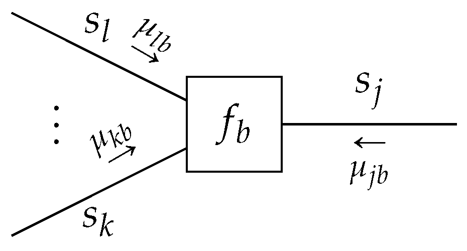
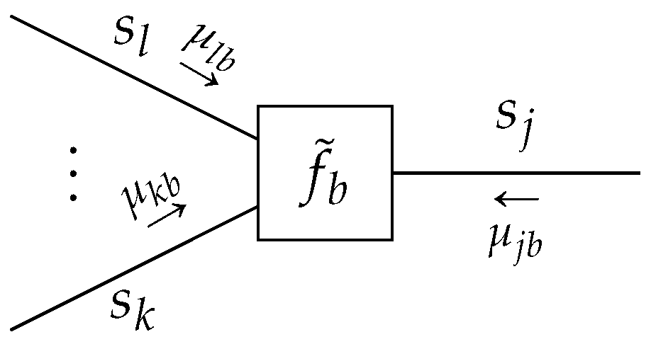
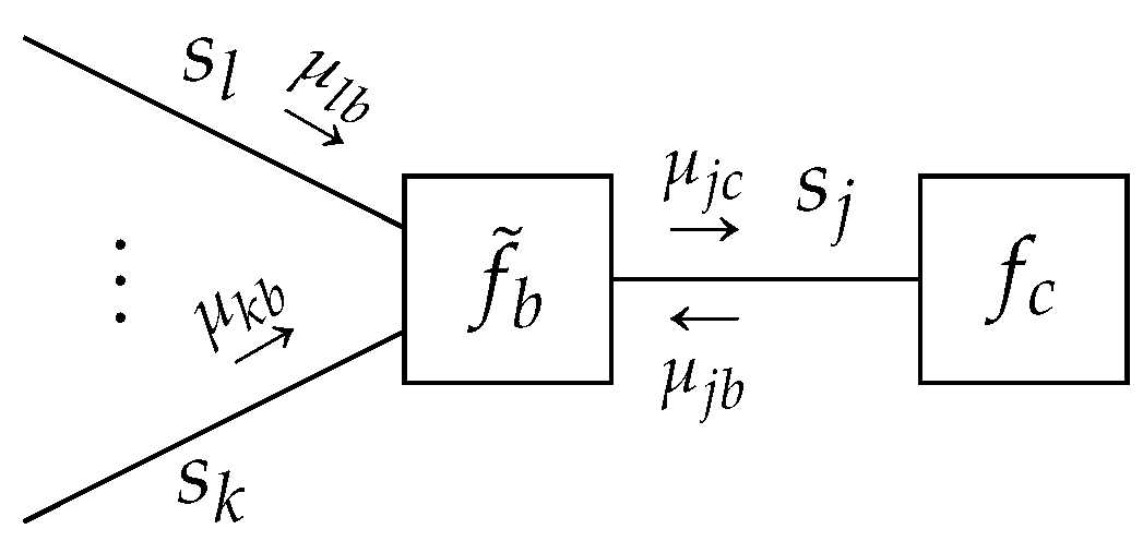
Given a TFFG$\mathcal{G}=(\mathcal{V},\mathcal{E})$, consider the node-induced subgraph$\mathcal{G}\left(b\right)$(Figure 3). The stationary points of the Lagrangian (16a) as a functional of $q_b$,

$$\begin{array}{cc}\hfill L_b[q_b,f_b]& =F[q_b,f_b]+{\psi }_b\left[\int q_b\left({\mathit{s}}_b\right)d{\mathit{s}}_b-1\right]+\sum _{i\in \mathcal{E}\left(b\right)}\int {\lambda }_{ib}\left(s_i\right)\left[q_i\left(s_i\right)-\int q_b\left({\mathit{s}}_b\right)d{s}_{b\setminus i}\right]d{s}_i+C_b,\hfill \end{array}$$

(17)

where $C_b$ collects all terms that are independent of $q_b$, which are of the form

$$q_b\left({\mathit{s}}_b\right)=\frac{{\displaystyle f_b\left({\mathit{s}}_b\right)\prod _{i\in \mathcal{E}\left(b\right)}{\mu }_{ib}\left(s_i\right)}}{{\displaystyle \int f_b\left({\mathit{s}}_b\right)\prod _{i\in \mathcal{E}\left(b\right)}{\mu }_{ib}\left(s_i\right)\mathrm{d}{\mathit{s}}_b}}.$$

(18)

Proof. 

See Appendix D.1. □

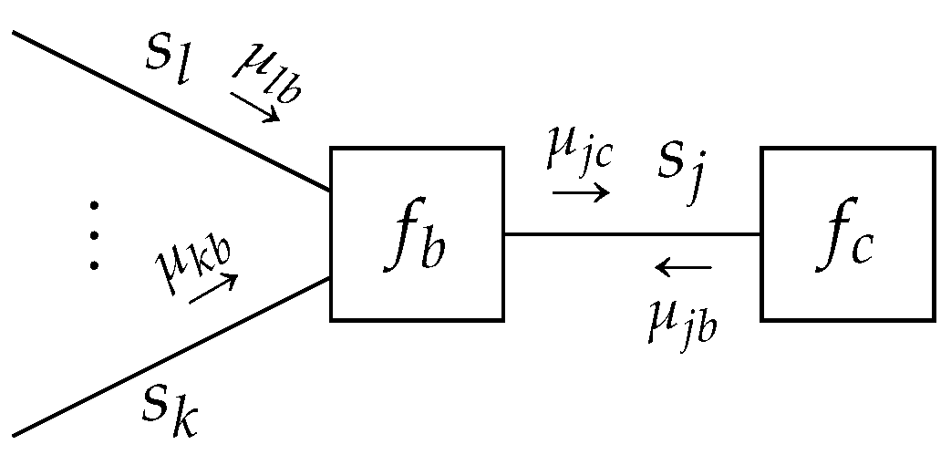
The ${\mu }_{ib}\left(s_i\right)$ are any set of positive functions that makes (18) satisfy (9b), and will be identified in Theorem 1.

Lemma 2.

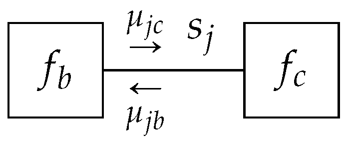
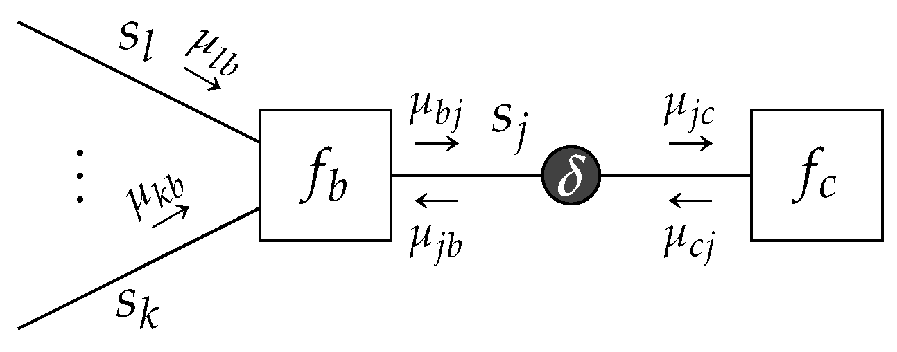
Given a TFFG$\mathcal{G}=(\mathcal{V},\mathcal{E})$, consider an edge-induced subgraph$\mathcal{G}\left(j\right)$(Figure 4). The stationary points of the Lagrangian (16b) as a functional of $q_j$,

$$\begin{array}{cc}\hfill L_j\left[q_j\right]& =H\left[q_j\right]+{\psi }_j\left[\int q_j\left(s_j\right)d{s}_j-1\right]+\sum _{a\in \mathcal{V}\left(j\right)}\int {\lambda }_{ja}\left(s_j\right)\left[q_j\left(s_j\right)-\int q_a\left({\mathit{s}}_a\right)d{s}_{a\setminus j}\right]d{s}_j+C_j,\hfill \end{array}$$

(19)

where $C_j$ collects all terms that are independent of $q_j$, are of the form

$$\begin{array}{cc}\hfill q_j\left(s_j\right)& =\frac{{\mu }_{jb}\left(s_j\right){\mu }_{jc}\left(s_j\right)}{{\displaystyle \int {\mu }_{jb}\left(s_j\right){\mu }_{jc}\left(s_j\right)\mathrm{d}{s}_j}}.\hfill \end{array}$$

(20)

Proof. 

See Appendix D.2. □

3.2. Minimizing the Bethe Free Energy by Belief Propagation

We now combine Lemmas 1 and 2 to derive the sum-product message update.

Theorem 1

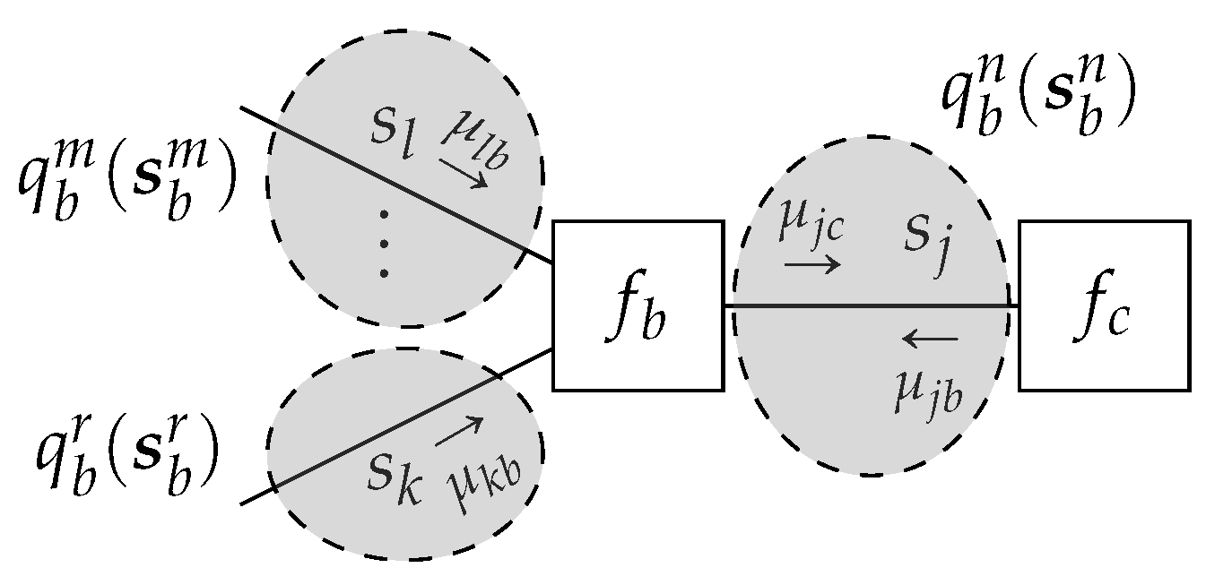
(Sum-Product Message Update). Given a TFFG $\mathcal{G}=(\mathcal{V},\mathcal{E})$, consider the induced subgraph $\mathcal{G}(b,j)$ (Figure 5). Given the local polytope $\mathcal{L}\left(\mathcal{G}\right(b,j\left)\right)$ of (14), then the local stationary solutions to (15) are given by

$$\begin{array}{cc}\hfill q_b^{*}\left({\mathit{s}}_b\right)& =\frac{{\displaystyle f_b\left({\mathit{s}}_b\right)\prod _{i\in \mathcal{E}\left(b\right)}{\mu }_{ib}^{*}\left(s_i\right)}}{{\displaystyle \int f_b\left({\mathit{s}}_b\right)\prod _{i\in \mathcal{E}\left(b\right)}{\mu }_{ib}^{*}\left(s_i\right)\mathrm{d}{\mathit{s}}_b}}\hfill \end{array}$$

(21a)

$$\begin{array}{cc}\hfill q_j^{*}\left(s_j\right)& =\frac{{\mu }_{jb}^{*}\left(s_j\right){\mu }_{jc}^{*}\left(s_j\right)}{{\displaystyle \int {\mu }_{jb}^{*}\left(s_j\right){\mu }_{jc}^{*}\left(s_j\right)\mathrm{d}{s}_j}},\hfill \end{array}$$

(21b)

with messages ${\mu }_{jc}^{*}\left(s_j\right)$ corresponding to the fixed points of

$$\begin{array}{cc}\hfill {\mu }_{jc}^{(k+1)}\left(s_j\right)& =\int f_b\left({\mathit{s}}_b\right)\prod _{\begin{array}{c}i\in \mathcal{E}\left(b\right)\\ i\ne j\end{array}}{\mu }_{ib}^{\left(k\right)}\left(s_i\right)\mathrm{d}{\mathit{s}}_{b\setminus j},\hfill \end{array}$$

(22)

with k representing an iteration index.

Proof. 

See Appendix D.3. □

The sum-product algorithm has proven to be useful in many engineering applications and disciplines. For example, it is widely used for decoding in communication systems [4,20,27]. Furthermore, for a linear Gaussian state space model, Kalman filtering and smoothing can be expressed in terms of sum-product message passing for state inference on a factor graph [28,29]. This equivalence has inspired applications ranging from localization [30] to estimation [31].

The sum-product algorithm with updates (22) obtains the exact Bayesian posterior when the underlying graph is a tree [24,25,32]. Application of the sum-product algorithm to cyclic graphs is not guaranteed to converge and might lead to oscillations in the BFE over iterations. Theorems 3.1 and 3.2 in [33] show that the BFE of a graph with a single cycle is convex, which implies that the sum-product algorithm will converge in this case. Moreover, ref. [19] shows that it is possible to obtain a double-loop message passing algorithm if the graph has a cycle such that the stable fixed points will correspond to local minima of the BFE.

Example 1.

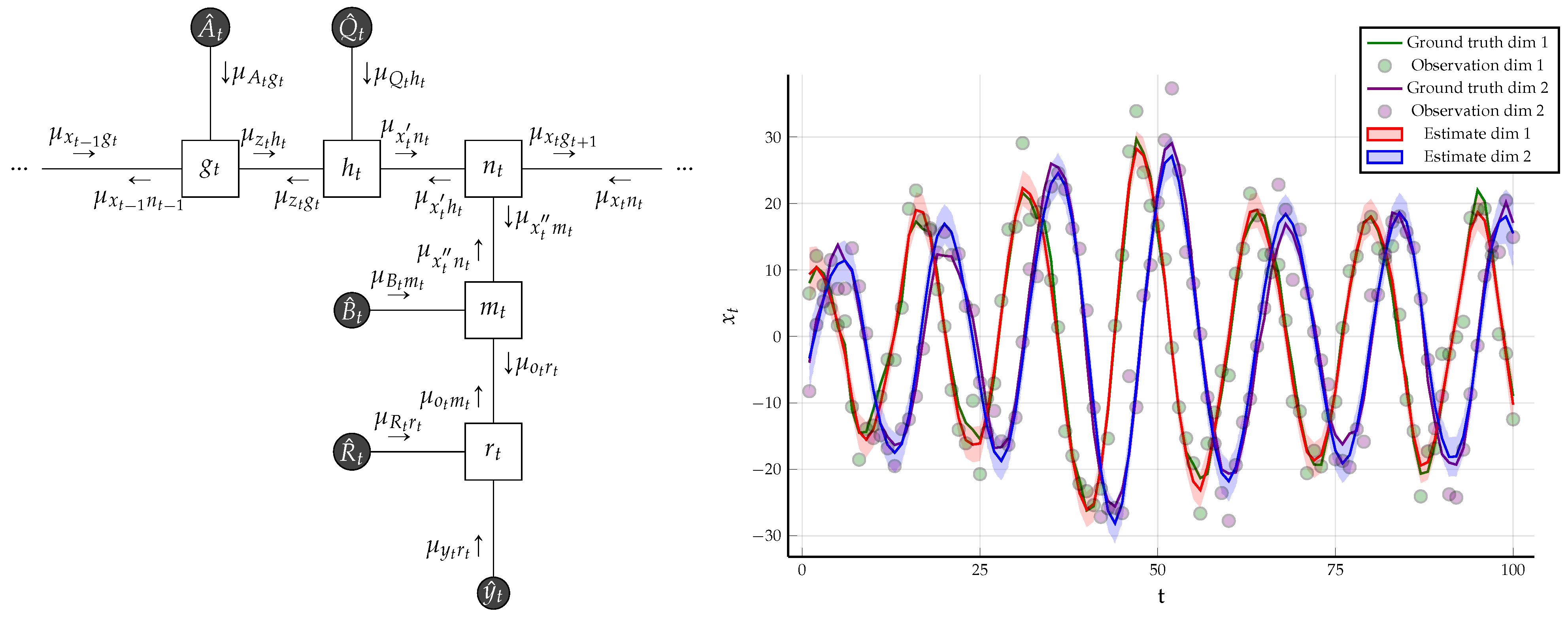
A Linear Dynamical System Considering a Linear Gaussian state space model specified by the following factors:

$$\begin{array}{cc}\hfill g_0\left(x_0\right)& =\mathcal{N}\left(x_0\right|m_{x_0},V_{x_0})\hfill \end{array}$$

(23a)

$$\begin{array}{cc}\hfill g_t(x_{t-1},z_t,A_t)& =\delta (z_t-A_t{x}_{t-1})\hfill \end{array}$$

(23b)

$$\begin{array}{cc}\hfill h_t(x_t^{\prime },z_t,Q_t)& =\mathcal{N}\left(x_t^{\prime }\right|z_t,Q_t^{-1})\hfill \end{array}$$

(23c)

$$\begin{array}{cc}\hfill n_t(x_t,x_t^{\prime },x_t^{\prime \prime })& =\delta (x_t-x_t^{\prime })\delta (x_t-x_t^{\prime \prime })\hfill \end{array}$$

(23d)

$$\begin{array}{cc}\hfill m_t(o_t,x_t^{″},B_t)& =\delta (o_t-B_t{x}_t^{″})\hfill \end{array}$$

(23e)

$$\begin{array}{cc}\hfill r_t(y_t,o_t,R_t)& =\mathcal{N}\left(y_t\right|o_t,R_t^{-1}).\hfill \end{array}$$

(23f)

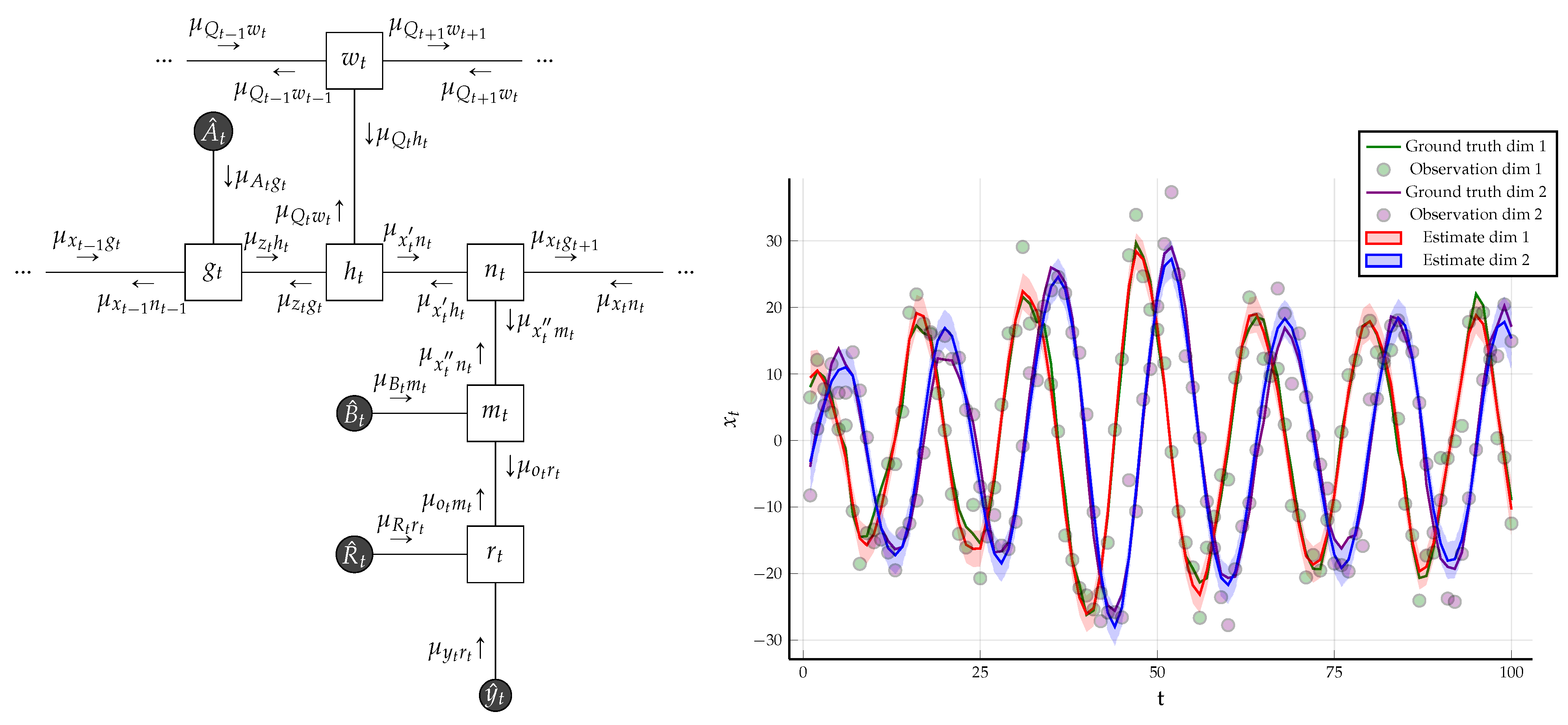
The FFG corresponding to the one time segment of the state space model is given in Figure 6. We assumed that we know the following matrices that are used to generate the data:

$$\begin{array}{cc}\hfill {\widehat{A}}_t& =\left[\begin{array}{cc}cos\left(\theta \right)& -sin\left(\theta \right)\\ sin\left(\theta \right)& cos\left(\theta \right)\end{array}\right],{\widehat{Q}}_t^{-1}=\left[\begin{array}{cc}3& 0.1\\ 0.1& 2\end{array}\right],{\widehat{B}}_t=\left[\begin{array}{cc}1& 0\\ 0& 1\end{array}\right],{\widehat{R}}_t^{-1}=\left[\begin{array}{cc}10& 2\\ 2& 20\end{array}\right]\hfill \end{array}$$

(24)

with$\theta =\pi /8$. Given a collection of observations$\widehat{\mathit{y}}=\{{\widehat{y}}_1,\dots ,{\widehat{y}}_T\}$, we constrain the latent states$\mathit{x}=\{x_0,\dots ,x_T\}$by local marginalization and normalization constraints (for brevity we omit writing the normalization constraints explicitly) in accordance with Theorem 1, i.e.,

$$\begin{array}{cc}\hfill \int q(x_{t-1},z_t,A_t)\mathrm{d}{x}_{t-1}\mathrm{d}{z}_t& =q\left(A_t\right),\int q(x_{t-1},z_t,A_t)\mathrm{d}{A}_t=q\left(z_t\right|x_{t-1})q\left(x_{t-1}\right)\hfill \end{array}$$

(25a)

$$\begin{array}{cc}\hfill \int q(x_t^{\prime },z_t,Q_t)\mathrm{d}{x}_t^{\prime }\mathrm{d}{z}_t& =q\left(Q_t\right),\int q(x_t^{\prime },z_t,Q_t)\mathrm{d}{z}_t\mathrm{d}{Q}_t=q\left(x_t^{\prime }\right),\int q(x_t^{\prime },z_t,Q_t)\mathrm{d}{x}_t^{\prime }\mathrm{d}{Q}_t=q\left(z_t\right)\hfill \end{array}$$

(25b)

$$\begin{array}{cc}\hfill q(x_t,x_t^{\prime },x_t^{″})& =q\left(x_t\right)\delta (x_t-x_t^{\prime })\delta (x_t-x_t^{″})\hfill \end{array}$$

(25c)

$$\begin{array}{cc}\hfill \int q(o_t,x_t^{″},B_t)\mathrm{d}{o}_t,\mathrm{d}{x}_t^{″}& =q\left(B_t\right),\int q(o_t,x_t^{″},B_t)\mathrm{d}{B}_t=q\left(o_t\right|x_t^{″})q\left(x_t^{″}\right)\hfill \end{array}$$

(25d)

$$\begin{array}{cc}\hfill \int q(o_t,y_t,R_t)\mathrm{d}{o}_t\mathrm{d}{y}_t& =q\left(R_t\right),\int q(o_t,y_t,R_t)\mathrm{d}{R}_t\mathrm{d}{o}_t=q\left(y_t\right),\int q(o_t,y_t,R_t)\mathrm{d}{R}_t\mathrm{d}{y}_t=q\left(o_t\right)\hfill \end{array}$$

(25e)

Moreover, we use data constraints in accordance with Theorem 3 (explained in Section 4.2.1) for the observations, state transition matrices and precision matrices, i.e.,

$$\begin{array}{c}\hfill q\left(y_t\right)=\delta (y_t-{\widehat{y}}_t),q\left(A_t\right)=\delta (A_t-{\widehat{A}}_t),q\left(B_t\right)=\delta (B_t-{\widehat{B}}_t),q\left(Q_t\right)=\delta (Q_t-{\widehat{Q}}_t),q\left(R_t\right)=\delta (R_t-{\widehat{R}}_t).\end{array}$$

Computation of sum-product messages by (22) is analytically tractable and detailed algebraic manipulation can be found in [31]. If the backwards messages are not passed, then the resulting sum-product message passing algorithm is equivalent to Kalman filtering and if both forward and backward messages are propagated, then the Rauch–Tung–Striebel smoother is obtained [34] (Ch. 8).

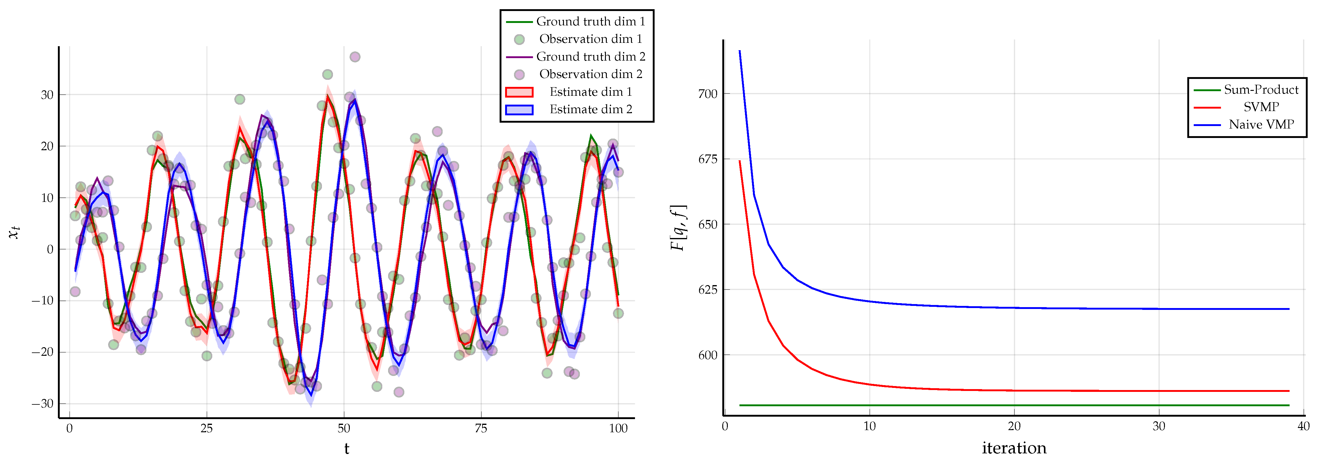
We generated$T=100$observations$\widehat{\mathit{y}}$using the matrices specified in (24) and the initial condition ${\widehat{x}}_0={[5,-5]}^{\top }$. Due to (23a), we have ${\mu }_{x_0{g}_1}=\mathcal{N}(m_{x_0},V_{x_0})$. We chose $V_{x_0}=100·\mathrm{I}$ and $m_{x_0}={\widehat{x}}_0$. Under these constraints, the results of sum-product message passing and Bethe free energy evaluation is given in Figure 6. As the underlying graph is a tree, sum-product message passing results are exact and the evaluated BFE corresponds to negative log-evidence. In the follow-up Example 2, we will modify the constraints and give a comparative free energy plot for the examples in Figures 10 and 16.

4. Message Passing Variations through Constraint Manipulation

For generic node functions with arbitrary connectivity, there is no guarantee that the sum-product updates can be solved analytically. When analytic solutions are not possible, there are two ways to proceed. One way is to try to solve the sum-product update equations numerically, e.g., by Monte Carlo methods. Alternatively, we can add additional constraints to the BFE that leads to simpler update equations at the cost of inference accuracy. In the remainder of the paper, we explore a variety of constraints that have proven to yield useful inference solutions.

4.1. Factorization Constraints

Additional factorizations of the variational density $q_a\left({\mathit{s}}_a\right)$ are often assumed to ease computation. In particular, we assumed a structured mean-field factorization such that

$$q_b\left({\mathit{s}}_b\right)\triangleq \prod _{n\in l\left(b\right)}{q}_b^n\left({\mathit{s}}_b^n\right),$$

(26)

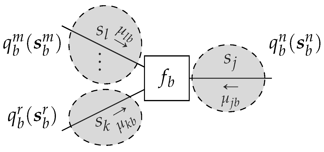
where n indicates a local cluster as a set of edges. To define a local cluster rigorously, let us first denote by $\mathcal{P}\left(a\right)$ the power set of an edge set $\mathcal{E}\left(a\right)$, where the power set is the set of all subsets of $\mathcal{E}\left(a\right)$. Then, a mean-field factorization $l\left(a\right)\subseteq \mathcal{P}\left(a\right)$ can be chosen such that all elements in $\mathcal{E}\left(a\right)$ are included in $l\left(a\right)$ exactly once. Therefore, $l\left(a\right)$ is defined as a set of one or multiple sets of edges. For example, if $\mathcal{E}\left(a\right)=\{i,j,k\}$, then $l\left(a\right)=\left\{\right\{i\},\{j,k\left\}\right\}$ is allowed, as is $l\left(a\right)=\left\{\right\{i,j,k\left\}\right\}$ itself, but $l\left(a\right)=\left\{\right\{i,j\},\{j,k\left\}\right\}$ is not allowed, since the element j occurs twice. More formally, in (26), the intersection of the super- and subscript collects the required variables, see Figure 7 for an example. The special case of a fully factorized $l\left(b\right)$ for all edges $i\in \mathcal{E}\left(b\right)$ is known as the naive mean-field factorization [11,24].

We will analyze the effect of a structured mean-field factorization (26) on the Bethe free energy (7) for a specific factor node $b\in \mathcal{V}$. Substituting (26) in the local free energy for factor b yields

$$F[q_b,f_b]=F[\left\{q_b^n\right\},f_b]=\sum _{n\in l\left(b\right)}\int q_b^n\left({\mathit{s}}_b^n\right)log{q}_b^n\left({\mathit{s}}_b^n\right)d{\mathit{s}}_b^n-\int \left\{\prod _{n\in l\left(b\right)}{q}_b^n\left({\mathit{s}}_b^n\right)\right\}log{f}_b\left({\mathit{s}}_b\right)d{\mathit{s}}_b.$$

(27)

We are then interested in

$$\begin{array}{cc}\hfill q_b^{m,*}& =arg\underset{q_b^m}{min}{L}_b^m[q_b^m,f_b],\hfill \end{array}$$

(28)

where the Lagrangian $L_b^m$ (Lemma 3) enforces the normalization and marginalization constraints

$$\begin{array}{cc}\hfill & \int q_b^m\left({\mathit{s}}_b^m\right)d{\mathit{s}}_b^m=1,\hfill \end{array}$$

(29a)

$$\begin{array}{cc}\hfill & \int q_b^m\left({\mathit{s}}_b^m\right)d{\mathit{s}}_{b\setminus i}^m=q_i\left(s_i\right),\mathrm{for}\mathrm{all}i\in m,m\in l\left(b\right).\hfill \end{array}$$

(29b)

Lemma 3.

Given a terminated FFG$\mathcal{G}=(\mathcal{V},\mathcal{E})$, consider a node-induced subgraph$\mathcal{G}\left(b\right)$with a structured mean-field factorization$l\left(b\right)$(e.g., Figure 7). Then, local stationary solutions to the Lagrangian

$$\begin{array}{cc}\hfill L_b^m\left[q_b^m\right]& =\int q_b^m\left({\mathit{s}}_b^m\right)log{q}_b^m\left({\mathit{s}}_b^m\right)d{\mathit{s}}_b^m-\int \left\{\prod _{n\in l\left(b\right)}{q}_b^n\left({\mathit{s}}_b^n\right)\right\}log{f}_b\left({\mathit{s}}_b\right)d{\mathit{s}}_b+\hfill \\ \hfill & {\psi }_b^m\left[\int q_b^m\left({\mathit{s}}_b^m\right)d{\mathit{s}}_b^m-1\right]+\sum _{i\in m}\int {\lambda }_{ib}\left(s_i\right)\left[q_i\left(s_i\right)-\int q_b^m\left({\mathit{s}}_b^m\right)d{\mathit{s}}_{m\setminus i}\right]d{s}_i+C_b^m,\hfill \end{array}$$

(30)

where$C_b^m$collects all terms independent of$q_b^m$, which are of the form

$$\begin{array}{cc}\hfill q_b^m\left({\mathit{s}}_b^m\right)& =\frac{{\displaystyle {\tilde{f}}_b^m\left({\mathit{s}}_b^m\right)\prod _{i\in m}{\mu }_{ib}\left(s_i\right)}}{{\displaystyle \int {\tilde{f}}_b^m\left({\mathit{s}}_b^m\right)\prod _{i\in m}{\mu }_{ib}\left(s_i\right)\mathrm{d}{\mathit{s}}_b^m}},\hfill \end{array}$$

(31)

where

$$\begin{array}{cc}\hfill {\tilde{f}}_b^m\left({\mathit{s}}_b^m\right)& =exp\left(\int \left\{\prod _{\begin{array}{c}n\in l\left(b\right)\\ n\ne m\end{array}}{q}_b^n\left({\mathit{s}}_b^n\right)\right\}log{f}_b\left({\mathit{s}}_b\right)d{\mathit{s}}_b^{\setminus m}\right).\hfill \end{array}$$

(32)

Proof. 

See Appendix D.4. □

4.1.1. Structured Variational Message Passing

We now combine Lemmas 2 and 3 to derive the structured variational message passing algorithm.

Theorem 2.

Structured variational message passing: Given a TFFG$\mathcal{G}=(\mathcal{V},\mathcal{E})$, consider the induced subgraph$\mathcal{G}(b,j)$with a structured mean-field factorization$l\left(b\right)\subseteq \mathcal{P}\left(b\right)$, with local clusters$n\in l\left(b\right)$. Let$m\in l\left(b\right)$be the cluster where$j\in m$(see, e.g., Figure 8). Given the local polytope

$$\begin{array}{c}\hfill \mathcal{L}\left(\mathcal{G}(b,j)\right)=\left\{q_b^{n}foralln\in l\left(b\right)s.t.\left(29\mathrm{a}\right),and{q}_{j}s.t.\left(29\mathrm{b}\right)\right\},\end{array}$$

(33)

then local stationary solutions to

$$\begin{array}{cc}\hfill \{q_b^{m,*},q_j^{*}\}& =arg\underset{\mathcal{L}\left(\mathcal{G}\right(b,j\left)\right)}{min}F[q,f],\hfill \end{array}$$

(34)

are given by

$$\begin{array}{cc}\hfill q_b^{m,*}\left({\mathit{s}}_b^m\right)& =\frac{{\tilde{f}}_b^{m,*}\left({\mathit{s}}_b^m\right){\prod }_{i\in m}{\mu }_{ib}^{*}\left(s_i\right)}{{\displaystyle \int {\tilde{f}}_b^{m,*}\left({\mathit{s}}_b^m\right)\prod _{i\in m}{\mu }_{ib}^{*}\left(s_i\right)\mathrm{d}{\mathit{s}}_b^m}}\hfill \end{array}$$

(35a)

$$\begin{array}{cc}\hfill q_j^{*}\left(s_j\right)& =\frac{{\mu }_{jb}^{*}\left(s_j\right){\mu }_{jc}^{*}\left(s_j\right)}{{\displaystyle \int {\mu }_{jb}^{*}\left(s_j\right){\mu }_{jc}^{*}\left(s_j\right)\mathrm{d}{s}_j}},\hfill \end{array}$$

(35b)

with messages${\mu }_{jc}^{*}\left(s_j\right)$corresponding to the fixed points of

$$\begin{array}{cc}\hfill {\mu }_{jc}^{(k+1)}\left(s_j\right)& =\int {\tilde{f}}_b^{m,\left(k\right)}\left({\mathit{s}}_b^m\right)\prod _{\begin{array}{c}i\in m\\ i\ne j\end{array}}{\mu }_{ib}^{\left(k\right)}\left(s_i\right)\mathrm{d}{\mathit{s}}_{b\setminus j}^m,\hfill \end{array}$$

(36)

with iteration index k, and where

$${\tilde{f}}_b^{m,\left(k\right)}=exp\left(\int \left\{\prod _{\begin{array}{c}n\in l\left(b\right)\\ n\ne m\end{array}}{q}_b^{n,\left(k\right)}\left({\mathit{s}}_b^n\right)\right\}log{f}_b\left({\mathit{s}}_b\right)d{\mathit{s}}_b^{\setminus m}\right).$$

(37)

Proof. 

See Appendix D.5. □

The structured mean-field factorization applies the marginalization constraint only to the local cluster beliefs, as opposed to the joint node belief. As a result, computation for the local cluster beliefs might become tractable [24] (Ch.5). The practical appeal of Variational Message Passing (VMP) based inference becomes evident when the underlying model is composed of conjugate factor pairs from the exponential family. When the underlying factors are conjugate exponential family distributions, the message passing updates (36) amounts to adding natural parameters [35] of the underlying exponential family distributions. Structured variational message passing is popular in acoustic signal modelling, e.g., [36], as it allows one to be able to keep track of correlations over time. In [37], a stochastic variant of structured variational inference is utilized for Latent Dirichlet Allocation. Structured approximations are also used to improve inference in auto-encoders. In [38], inference involving non-parametric Beta-Bernoulli process priors is improved by developing a structured approximation to variational auto-encoders. When the data being modelled are time series, structured approximations reflect the transition structure over time. In [39], an efficient structured black-box variational inference algorithm for fitting Gaussian variational models to latent time series is proposed.

Example 2.

Consider the linear Gaussian state space model of Example 1. Let us assume that the precision matrix for latent-state transitions$Q_t$is not known and can not be constrained by data. Then, we can augment state space model by including a prior for$Q_t$and try to infer a posterior over$Q_t$from the observations. Since$Q_t$is the precision of a normal factor, we chose a conjugate Wishart prior and assumed that$Q_t$is time-invariant by adding the following factors

$$\begin{array}{cc}\hfill w_0(Q_0,V,\nu )& =\mathcal{W}\left(Q_0\right|V,\nu )\hfill \end{array}$$

(38a)

$$\begin{array}{cc}\hfill w_t(Q_{t-1},Q_t,Q_{t+1})& =\delta (Q_{t-1}-Q_t)\delta (Q_t-Q_{t+1}),foreveryt=1,\dots ,T.\hfill \end{array}$$

(38b)

It is certainly possible to assume a time-varying structure for$Q_t$; however, our purpose is to illustrate a change in constraints rather than analyzing time-varying properties. This is why we assume time-invariance.

In this setting, the sum-product equations around the factor$h_t$are not analytically tractable. Therefore, we changed the constraints associated with$h_t$ (25b) to those given in Theorem 2 as follows

$$\begin{array}{cc}\hfill \int q(x_t^{\prime },z_t,Q_t)\mathrm{d}{x}_t^{\prime }\mathrm{d}{z}_t& =q\left(Q_t\right),\int q(x_t^{\prime },z_t,Q_t)\mathrm{d}{Q}_t=q(x_t^{\prime },z_t)\hfill \end{array}$$

(39a)

$$\begin{array}{cc}\hfill \int q\left(Q_t\right)\mathrm{d}{Q}_t& =1,\int q(x_t^{\prime },z_t)\mathrm{d}{x}_t^{\prime }\mathrm{d}{z}_t=1.\hfill \end{array}$$

(39b)

We removed the data constraint on $q\left(Q_t\right)$ and instead included data constraints on the hyper-parameters

$$\begin{array}{c}\hfill q\left(V\right)=\delta (V-\widehat{V}),q\left(\nu \right)=\delta (\nu -\widehat{\nu }).\end{array}$$

(40)

With the new set of constraints ((39a) and (39b)), we obtained a hybrid of the sum-product and structured VMP algorithm, where structured messages around the factor $h_t$ are computed by (36) and the rest of the messages are computed by the sum-product (22). One time segment of the modified FFG along with the messages is given Figure 9. We used the same observations $\widehat{\mathit{y}}$ that were generated in Example 1 and the same initialization for the hidden states. For the hyper-parameters of the Wishart prior, we chose $\widehat{V}=0.1·\mathrm{I}$ and $\widehat{\nu }=2$. Under these constraints, the result of structured variational message passing results along with the Bethe free energy evaluation is given in Figure 9.

4.1.2. Naive Variational Message Passing

As a corollary of Theorem 2, we can consider the special case of a naive mean-field factorization, which is defined for node b as

$$\begin{array}{c}\hfill q_b\left({\mathit{s}}_b\right)=\prod _{i\in \mathcal{E}\left(b\right)}{q}_i\left(s_i\right).\end{array}$$

(41)

The naive mean-field constraint (41) transforms the local free energy into

$$\begin{array}{cc}\hfill F[q_b,f_b]& =F[\left\{q_i\right\},f_b]\hfill \\ \hfill & =\sum _{i\in \mathcal{E}\left(b\right)}\int q_i\left(s_i\right)log{q}_i\left(s_i\right)d{s}_i-\int \left\{\prod _{i\in \mathcal{E}\left(b\right)}{q}_i\left(s_i\right)\right\}log{f}_b\left({\mathit{s}}_b\right)d{\mathit{s}}_b.\hfill \end{array}$$

(42)

Corollary 1.

Naive Variational Message Passing: Given a TFFG $\mathcal{G}=(\mathcal{V},\mathcal{E})$, consider the induced subgraph $\mathcal{G}(b,j)$ with a naive mean-field factorization $l\left(b\right)=\{i\mathrm{such}\mathrm{that}\mathrm{for}\mathrm{all}i\in \mathcal{E}(b\left)\right\}$. Let $m\in l\left(b\right)$ be the cluster where $j=m$. Given the local polytope of (33), the local stationary solutions to (34) are given by

$$\begin{array}{cc}\hfill q_b^{m,*}\left({\mathit{s}}_b^m\right)& =q_j^{*}\left(s_j\right)=\frac{{\mu }_{jb}^{*}\left(s_j\right){\mu }_{jc}^{*}\left(s_j\right)}{{\displaystyle \int {\mu }_{jb}^{*}\left(s_j\right){\mu }_{jc}^{*}\left(s_j\right)d{s}_j}},\hfill \end{array}$$

where the messages ${\mu }_{jc}^{*}\left(s_j\right)$ are the fixed points of the following iterations

$$\begin{array}{cc}\hfill {\mu }_{jc}^{(k+1)}\left(s_j\right)& =exp\left(\int \left\{\prod _{\begin{array}{c}i\in \mathcal{E}\left(b\right)\\ i\ne j\end{array}}{q}_i^{\left(k\right)}\left(s_i\right)\right\}log{f}_b\left({\mathit{s}}_b\right)d{\mathit{s}}_{b\setminus j}\right),\hfill \end{array}$$

(43)

where k is an iteration index.

Proof. 

See Appendix D.6. □

The naive mean-field factorization limits the search space of beliefs by imposing strict constraints on the variational posterior. As a result, the variational posterior also loses flexibility. To improve inference performance for sparse Bayesian learning, the authors of [40] proposes a hybrid mechanism by augmenting naive mean-field VMP with sum-product updates. This hybrid scheme reduces the complexity of the sum-product algorithm, while improving the accuracy of the naive VMP approach. In [41], naive VMP is applied to semi-parametric regression and allows for scaling of regression models to large data sets.

Example 3.

As a follow up on Example 2, we relaxed the constraints in ((39a) and (39b)) to the following constraints presented in Corollary 1 as

$$\begin{array}{cc}\hfill \int q(x_t^{\prime },z_t,Q_t)\mathrm{d}{x}_t^{\prime }\mathrm{d}{z}_t& =q\left(Q_t\right),\int q(x_t^{\prime },z_t,Q_t)\mathrm{d}{Q}_t=q(x_t^{\prime },z_t)=q\left(x_t^{\prime }\right)q\left(z_t\right)\hfill \end{array}$$

(44a)

$$\begin{array}{cc}\hfill \int q\left(Q_t\right)\mathrm{d}{Q}_t& =1,\int q\left(x_t^{\prime }\right)\mathrm{d}{x}_t^{\prime }=1,\int q\left(z_t\right)\mathrm{d}{z}_t=1.\hfill \end{array}$$

(44b)

The FFG remains the same and we use identical data constraints as in Example 2. Together with constraint (44), we obtained a hybrid of naive variational message passing and sum-product message passing algorithm where the messages around the factor $h_t$ are computed by (43) and the rest of the messages by sum-product (22). Using the same data as in Example 1, the results for naive VMP are given in Figure 10 along with the evaluated Bethe free energy.

4.2. Form Constraints

Form constraints limit the functional form of the variational factors $q_a\left({\mathit{s}}_a\right)$ and $q_i\left(s_i\right)$. One of the most widely used form constraints, the data constraint, is also illustrated in Appendix A.

4.2.1. Data Constraints

A data constraint can be viewed as a special case of (9b), where the belief $q_j$ is constrained to be a Dirac-delta function [42], such that

$$\begin{array}{c}\hfill \int q_a\left({\mathit{s}}_a\right)d{\mathit{s}}_{a\setminus j}=q_j\left(s_j\right)=\delta (s_j-{\widehat{s}}_j),\end{array}$$

(45)

where ${\widehat{s}}_j$ is a known value, e.g., an observation.

Lemma 4.

Given a TFFG$\mathcal{G}=(\mathcal{V},\mathcal{E})$, consider the node-induced subgraph$\mathcal{G}\left(b\right)$(Figure 3). Then local stationary solutions to the Lagrangian

$$\begin{array}{cc}\hfill L_b[q_b,f_b]& =F[q_b,f_b]+{\psi }_b\left[\int q_b\left({\mathit{s}}_b\right)d{\mathit{s}}_b-1\right]+\sum _{\begin{array}{c}i\in \mathcal{E}\left(b\right)\\ i\ne j\end{array}}\int {\lambda }_{ib}\left(s_i\right)\left[q_i\left(s_i\right)-\int q_b\left({\mathit{s}}_b\right)d{s}_{b\setminus i}\right]d{s}_i+\hfill \\ \hfill & \int {\lambda }_{jb}\left(s_j\right)\left[\delta (s_j-{\widehat{s}}_j)-\int q_b\left({\mathit{s}}_b\right)d{s}_{b\setminus j}\right]d{s}_j+C_b.\hfill \end{array}$$

(46)

where$C_b$collects all terms that are independent of$q_b$, are of the form

$$\begin{array}{cc}\hfill q_b\left({\mathit{s}}_b\right)& =\frac{{\displaystyle f_b\left({\mathit{s}}_b\right)\prod _{i\in \mathcal{E}\left(b\right)}{\mu }_{ib}\left(s_i\right)}}{{\displaystyle \int f_b\left({\mathit{s}}_b\right)\prod _{i\in \mathcal{E}\left(b\right)}{\mu }_{ib}\left(s_i\right)\mathrm{d}{\mathit{s}}_b}}.\hfill \end{array}$$

(47)

Proof. 

See Appendix D.7. □

Theorem 3.

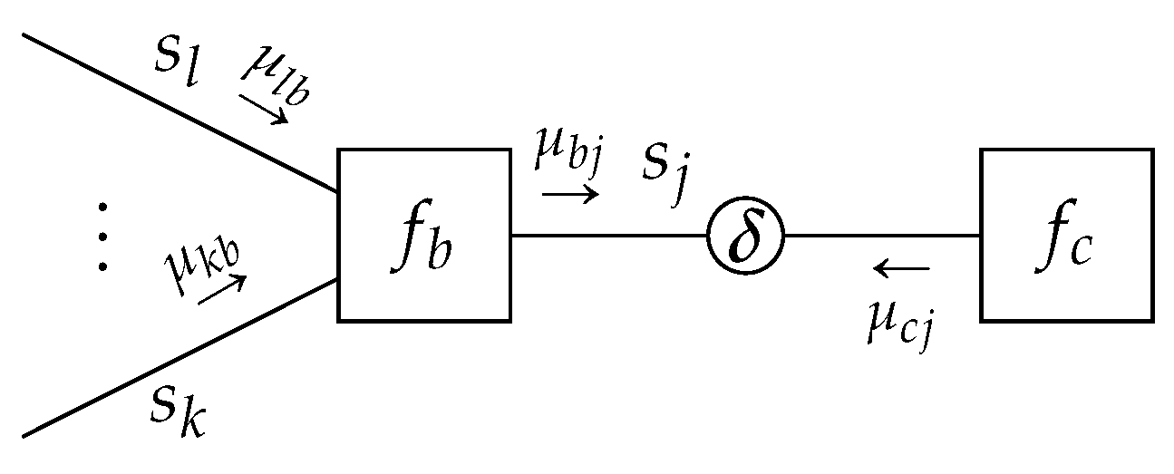
Data-Constrained Sum-Product: Given a TFFG$\mathcal{G}=(\mathcal{V},\mathcal{E})$, consider the induced subgraph$\mathcal{G}(b,j)$(Figure 11). Given the local polytope

$$\begin{array}{c}\hfill \mathcal{L}\left(\mathcal{G}(b,j)\right)=\left\{q_{b}s.t.\right(45\left)\right\},\end{array}$$

(48)

the local stationary solutions to

$$\begin{array}{c}\hfill q_b^{*}=arg\underset{\mathcal{L}\left(\mathcal{G}\right(b,j\left)\right)}{min}F[q,f],\end{array}$$

are of the form

$$\begin{array}{cc}\hfill q_b^{*}\left({\mathit{s}}_b\right)& =\frac{{\displaystyle f_b\left({\mathit{s}}_b\right)\prod _{i\in \mathcal{E}\left(b\right)}{\mu }_{ib}^{*}\left(s_i\right)}}{{\displaystyle \int f_b\left({\mathit{s}}_b\right)\prod _{i\in \mathcal{E}\left(b\right)}{\mu }_{ib}^{*}\left(s_i\right)\mathrm{d}{\mathit{s}}_b}},\hfill \end{array}$$

(49)

with message

$$\begin{array}{cc}\hfill {\mu }_{jb}^{*}\left(s_j\right)& =\delta (s_j-{\widehat{s}}_j).\hfill \end{array}$$

(50)

Proof. 

See Appendix D.8. □

Note that the resulting message ${\mu }_{jb}^{*}\left(s_j\right)$ to node b does not depend on messages from node c, as would be the case for a sum-product update. By the symmetry of Theorem 3 for the subgraph $\mathcal{L}\left\{\mathcal{G}\right(c,j\left)\right\}$, (A32) identifies

$$\begin{array}{c}\hfill {\mu }_{cj}\left(s_j\right)=\int f_c\left({\mathit{s}}_c\right)\prod _{\begin{array}{c}i\in \mathcal{E}\left(c\right)\\ i\ne j\end{array}}{\mu }_{ic}\left(s_i\right)d{\mathit{s}}_{c\setminus j}\ne \delta (s_j-{\widehat{s}}_j).\end{array}$$

This implies that messages incoming to a data constraint (such as ${\mu }_{cj}$) are not further propagated through the data constraint. The data constraint thus effectively introduces a conditional independence between the variables of neighboring factors (conditioned on the shared constrained variable). Interestingly, this is similar to the notion of an intervention [43], where a decision variable is externally forced to a realization.

Data constraints allow information from data sets to be absorbed into the model. Essentially, (variational) Bayesian machine learning is an application of inference in a graph with data constraints. In our framework, data are a constraint, and machine learning via Bayes rule follows naturally from the minimization of the Bethe free energy (see also Appendix A).

4.2.2. Laplace Propagation

A second type of form constraint we consider is the Laplace constraint, see also [14]. Consider a second-order Taylor approximation on the local log-node function

$$\begin{array}{c}\hfill {\mathcal{L}}_a\left({\mathit{s}}_a\right)=log{f}_a\left({\mathit{s}}_a\right),\end{array}$$

(51)

around an approximation point ${\widehat{\mathit{s}}}_a$, as

$$\begin{array}{c}\hfill {\tilde{\mathcal{L}}}_a({\mathit{s}}_a;{\widehat{\mathit{s}}}_a)={\mathcal{L}}_a\left({\widehat{\mathit{s}}}_a\right)+{\nabla }^{\top }{\mathcal{L}}_a\left({\widehat{\mathit{s}}}_a\right)\left({\mathit{s}}_a-{\widehat{\mathit{s}}}_a\right)+\frac{1}{2}{\left({\mathit{s}}_a-{\widehat{\mathit{s}}}_a\right)}^{\top }{\nabla }^2{\mathcal{L}}_a\left({\widehat{\mathit{s}}}_a\right)\left({\mathit{s}}_a-{\widehat{\mathit{s}}}_a\right).\end{array}$$

(52)

From this approximation, we define the Laplace-approximated node function as

$$\begin{array}{cc}\hfill {\tilde{f}}_a({\mathit{s}}_a;{\widehat{\mathit{s}}}_a)& \triangleq exp\left({\tilde{\mathcal{L}}}_a({\mathit{s}}_a;{\widehat{\mathit{s}}}_a)\right),\hfill \end{array}$$

(53)

which is substituted in the local free energy to obtain the Laplace-encoded local free energy as

$$\begin{array}{cc}\hfill F[q_a,{\tilde{f}}_a;{\widehat{\mathit{s}}}_a]& =\int q_a\left({\mathit{s}}_a\right)log\frac{q_a\left({\mathit{s}}_a\right)}{{\tilde{f}}_a({\mathit{s}}_a;{\widehat{\mathit{s}}}_a)}d{\mathit{s}}_a.\hfill \end{array}$$

(54)

It follows that the Laplace-encoded optimization of the local free energy becomes

$$\begin{array}{cc}\hfill q_a^{*}& =arg\underset{q_a}{min}{L}_a[q_a,{\tilde{f}}_a;{\widehat{\mathit{s}}}_a],\hfill \end{array}$$

(55)

where the Lagrangian $L_a$ imposes the marginalization and normalization constraints of (9) on (54).

Lemma 5.

Given a TFFG$\mathcal{G}=(\mathcal{V},\mathcal{E})$, consider the node-induced subgraph$\mathcal{G}\left(b\right)$(Figure 12). The stationary points of the Laplace-approximated Lagrangian (55) as a functional of $q_b$,

$$\begin{array}{cc}\hfill L_b[q_b,{\tilde{f}}_b;{\widehat{\mathit{s}}}_b]& =F[q_b,{\tilde{f}}_b;{\widehat{\mathit{s}}}_b]+{\psi }_b\left[\int q_b\left({\mathit{s}}_b\right)d{\mathit{s}}_b-1\right]+\hfill \\ \hfill & \sum _{i\in \mathcal{E}\left(b\right)}\int {\lambda }_{ib}\left(s_i\right)\left[q_i\left(s_i\right)-\int q_b\left({\mathit{s}}_b\right)d{s}_{b\setminus i}\right]d{s}_i+C_b,\hfill \end{array}$$

(56)

where $C_b$ collects all terms that are independent of $q_b$, which are of the form

$$q_b\left({\mathit{s}}_b\right)=\frac{{\displaystyle {\tilde{f}}_b({\mathit{s}}_b;{\widehat{\mathit{s}}}_b)\prod _{i\in \mathcal{E}\left(b\right)}{\mu }_{ib}\left(s_i\right)}}{{\displaystyle \int {\tilde{f}}_b({\mathit{s}}_b;{\widehat{\mathit{s}}}_b)\prod _{i\in \mathcal{E}\left(b\right)}{\mu }_{ib}\left(s_i\right)\mathrm{d}{\mathit{s}}_b}}.$$

(57)

Proof. 

See Appendix D.9. □

We can now formulate Laplace propagation as an iterative procedure, where the approximation point ${\widehat{\mathit{s}}}_b$ is chosen as the mode of the belief $q_b\left({\mathit{s}}_b\right)$.

Theorem 4.

Laplace Propagation: Given a TFFG$\mathcal{G}=(\mathcal{V},\mathcal{E})$, consider the induced subgraph$\mathcal{G}(b,j)$(Figure 13) with the Laplace-encoded factor${\tilde{f}}_b$as per (53). We write the model (1) with the Laplace-encoded factor ${\tilde{f}}_b$ substituted for $f_b$, as $\tilde{f}$. Given the local polytope $\mathcal{L}\left(\mathcal{G}\right(b,j\left)\right)$ of (14), the local stationary solutions to

$$\begin{array}{cc}\hfill \{q_b^{*},q_j^{*}\}& =arg\underset{\mathcal{L}\left(\mathcal{G}\right(b,j\left)\right)}{min}F[q,\tilde{f};{\widehat{\mathit{s}}}_b],\hfill \end{array}$$

(58)

are given by

$$\begin{array}{cc}\hfill q_b^{*}\left({\mathit{s}}_b\right)& =\frac{{\displaystyle {\tilde{f}}_b({\mathit{s}}_b;{\widehat{\mathit{s}}}_b^{*})\prod _{i\in \mathcal{E}\left(b\right)}{\mu }_{ib}^{*}\left(s_i\right)}}{{\displaystyle \int {\tilde{f}}_b({\mathit{s}}_b;{\widehat{\mathit{s}}}_b^{*})\prod _{i\in \mathcal{E}\left(b\right)}{\mu }_{ib}^{*}\left(s_i\right)\mathrm{d}{\mathit{s}}_b}}\hfill \\ \hfill q_j^{*}\left(s_j\right)& =\frac{{\mu }_{jb}^{*}\left(s_j\right){\mu }_{jc}^{*}\left(s_j\right)}{{\displaystyle \int {\mu }_{jb}^{*}\left(s_j\right){\mu }_{jc}^{*}\left(s_j\right)\mathrm{d}{s}_j}},\hfill \end{array}$$

with ${\widehat{\mathit{s}}}_b^{*}$ and the messages ${\mu }_{jc}^{*}\left(s_j\right)$ the fixed points of

$$\begin{array}{cc}\hfill {\widehat{\mathit{s}}}_b^{\left(k\right)}& =arg\underset{{\mathit{s}}_b}{max}log{q}_b^{\left(k\right)}\left({\mathit{s}}_b\right)\hfill \\ \hfill q_b^{(k+1)}\left({\mathit{s}}_b\right)& =\frac{{\displaystyle {\tilde{f}}_b({\mathit{s}}_b;{\widehat{\mathit{s}}}_b^{\left(k\right)})\prod _{i\in \mathcal{E}\left(b\right)}{\mu }_{ib}^{\left(k\right)}\left(s_i\right)}}{{\displaystyle \int {\tilde{f}}_b({\mathit{s}}_b;{\widehat{\mathit{s}}}_b^{\left(k\right)})\prod _{i\in \mathcal{E}\left(b\right)}{\mu }_{ib}^{\left(k\right)}\left(s_i\right)\mathrm{d}{\mathit{s}}_b}}\hfill \\ \hfill {\mu }_{jc}^{(k+1)}\left(s_j\right)& =\int {\tilde{f}}_b({\mathit{s}}_b;{\widehat{\mathit{s}}}_b^{\left(k\right)})\prod _{\begin{array}{c}i\in \mathcal{E}\left(b\right)\\ i\ne j\end{array}}{\mu }_{ib}^{\left(k\right)}\left(s_i\right)\mathrm{d}{\mathit{s}}_{b\setminus j}.\hfill \end{array}$$

Proof. 

See Appendix D.10. □

A Laplace propagation is introduced in [14] as an algorithm that propagates mean and variance information when exact updates are expensive to compute. Laplace propagation has found applications in the context of Gaussian processes and support vector machines [14]. In the jointly normal case, Laplace propagation coincides with sum-product and expectation propagation [14,18].

4.2.3. Expectation Propagation

Expectation propagation can be derived in terms of constraint manipulation by relaxing the marginalization constraints to expectation constraints. Expectation constraints are of the form

$$\begin{array}{c}\hfill \int q_a\left({\mathit{s}}_a\right)T_i\left(s_i\right)\mathrm{d}{\mathit{s}}_a=\int q_i\left(s_i\right)T_i\left(s_i\right)\mathrm{d}{s}_i,\end{array}$$

(59)

for a given function (statistic) $T_i\left(s_i\right)$. Technically, the statistic $T_i\left(s_i\right)$ can be chosen arbitrarily. Nevertheless, they are often chosen as sufficient statistics of an exponential family distribution. An exponential family distribution is defined by

$$q_i\left(s_i\right)=h\left(s_i\right)exp\left({\eta }_i^{\top }{T}_i\left(s_i\right)-logZ\left({\eta }_i\right)\right),$$

(60)

where ${\eta }_i$ is the natural parameter, $Z\left({\eta }_i\right)$ is the partition function, $T_i\left(s_i\right)$ is the sufficient statistics and $h\left(s_i\right)$ is a base measure [24]. The reason $T_i\left(s_i\right)$ is a sufficient statistic is because if there are observed values of the random variable $s_i$, then the parameter ${\eta }_i$ can be estimated by using only the statistics $T_i\left(s_i\right)$. This means that the estimator of ${\eta }_i$ will depend only on the statistics.

The idea behind expectation propagation [18] is to relax the marginalization constraints with moment-matching constraints by choosing sufficient statistics from exponential family distributions [12]. Relaxation allows approximating the marginals of the sum-product algorithm with exponential family distributions. By keeping the marginals within the exponential family, the complexity of the resulting computations is reduced.

Lemma 6.

Given a TFFG$\mathcal{G}=(\mathcal{V},\mathcal{E})$, consider the node-induced subgraph$\mathcal{G}\left(b\right)$(Figure 3). The stationary points of the Lagrangian

$$\begin{array}{cc}\hfill L_b[q_b,f_b]& =F[q_b,f_b]+{\psi }_b\left[\int q_b\left({\mathit{s}}_b\right)d{\mathit{s}}_b-1\right]+\sum _{\begin{array}{c}i\in \mathcal{E}\left(b\right)\\ i\ne j\end{array}}\int {\lambda }_{ib}\left(s_i\right)\left[q_i\left(s_i\right)-\int q_b\left({\mathit{s}}_b\right)d{s}_{b\setminus i}\right]d{s}_i+\hfill \end{array}$$

$$\begin{array}{c}\hfill {\eta }_{jb}^{\top }\left[\int q_j\left(s_j\right)T_j\left(s_j\right)\mathrm{d}{s}_j-\int q_b\left({\mathit{s}}_b\right)T_j\left(s_j\right)\mathrm{d}{\mathit{s}}_b\right]+C_b,\end{array}$$

(61)

with sufficient statistics$T_j$, and where$C_b$collects all terms that are independent of$q_b$, are of the form

$$\begin{array}{cc}\hfill q_b\left({\mathit{s}}_b\right)& =\frac{{\displaystyle f_b\left({\mathit{s}}_b\right)\prod _{i\in \mathcal{E}\left(b\right)}{\mu }_{ib}\left(s_i\right)}}{{\displaystyle \int f_b\left({\mathit{s}}_b\right)\prod _{i\in \mathcal{E}\left(b\right)}{\mu }_{ib}\left(s_i\right)\mathrm{d}{\mathit{s}}_b}},\hfill \end{array}$$

(62)

with incoming exponential family message

$$\begin{array}{cc}\hfill {\mu }_{jb}\left(s_j\right)& =exp\left({\eta }_{jb}^{\top }{T}_j\left(s_j\right)\right).\hfill \end{array}$$

(63)

Proof. 

See Appendix D.11. □

Lemma 7.

Given a TFFG $\mathcal{G}=(\mathcal{V},\mathcal{E})$, consider an edge-induced subgraph $\mathcal{G}\left(j\right)$ (Figure 4). The stationary solutions of the Lagrangian

$$\begin{array}{cc}\hfill L_j\left[q_j\right]& =H\left[q_j\right]+{\psi }_j\left[\int q_j\left(s_j\right)d{s}_j-1\right]+\sum _{a\in \mathcal{V}\left(j\right)}{\eta }_{ja}^{\top }\left[\int q_j\left(s_j\right)T_j\left(s_j\right)\mathrm{d}{s}_j-\int q_a\left({\mathit{s}}_a\right)T_j\left(s_j\right)\mathrm{d}{\mathit{s}}_a\right]+C_j,\hfill \end{array}$$

with sufficient statistics $T_j\left(s_j\right)$, and where $C_j$ collects all terms that are independent of $q_j$, are of the form

$$\begin{array}{cc}\hfill q_j\left(s_j\right)& =\frac{exp\left({[{\eta }_{jb}+{\eta }_{jc}]}^{\top }{T}_j\left(s_j\right)\right)}{{\displaystyle \int exp\left({[{\eta }_{jb}+{\eta }_{jc}]}^{\top }{T}_j\left(s_j\right)\right)\mathrm{d}{s}_j}}.\hfill \end{array}$$

(64)

Proof. 

See Appendix D.12. □

Theorem 5.

Expectation Propagation: Given a TFFG$\mathcal{G}=(\mathcal{V},\mathcal{E})$, consider the induced subgraph$\mathcal{G}(b,j)$(Figure 5). Given the local polytope

$$\begin{array}{c}\hfill \mathcal{L}\left(\mathcal{G}(b,j)\right)=\left\{q_{b}s.t.\left(9\mathrm{a}\right),and{q}_{j}s.t.\left(59\right)and\left(10\right)\right\},\end{array}$$

(65)

and${\mu }_{jb}\left(s_j\right)=exp\left({\eta }_{jb}^{\top }{T}_j\left(s_j\right)\right)$an exponential family message (from Lemma 6). Then, the local stationary solutions to (15) are given by

$$\begin{array}{cc}\hfill q_b^{*}\left({\mathit{s}}_b\right)& =\frac{{\displaystyle f_b\left({\mathit{s}}_b\right)\prod _{i\in \mathcal{E}\left(b\right)}{\mu }_{ib}^{*}\left(s_i\right)}}{{\displaystyle \int f_b\left({\mathit{s}}_b\right)\prod _{i\in \mathcal{E}\left(b\right)}{\mu }_{ib}^{*}\left(s_i\right)\mathrm{d}{\mathit{s}}_b}}\hfill \end{array}$$

(66a)

$$\begin{array}{cc}\hfill q_j^{*}\left(s_j\right)& =\frac{exp\left({[{\eta }_{jb}^{*}+{\eta }_{jc}^{*}]}^{\top }{T}_j\left(s_j\right)\right)}{{\displaystyle \int exp\left({[{\eta }_{jb}^{*}+{\eta }_{jc}^{*}]}^{\top }{T}_j\left(s_j\right)\right)\mathrm{d}{s}_j}},\hfill \end{array}$$

(66b)

with ${\eta }_{jb}^{*},{\eta }_{jc}^{*}$ and ${\mu }_{jc}^{*}\left(s_j\right)$ being the fixed points of the iterations

$$\begin{array}{cc}\hfill {\tilde{\mu }}_{jc}^{\left(k\right)}\left(s_j\right)& =\int f_b\left({\mathit{s}}_b\right)\prod _{\begin{array}{c}i\in \mathcal{E}\left(b\right)\\ i\ne j\end{array}}{\mu }_{ib}^{\left(k\right)}\left(s_i\right)d{\mathit{s}}_{b\setminus j}\hfill \\ \hfill {\tilde{q}}_j^{\left(k\right)}\left(s_j\right)& =\frac{{\mu }_{jb}^{\left(k\right)}\left(s_j\right){\tilde{\mu }}_{jc}^{\left(k\right)}\left(s_j\right)}{{\displaystyle \int {\mu }_{jb}^{\left(k\right)}\left(s_j\right){\tilde{\mu }}_{jc}^{\left(k\right)}\left(s_j\right)\mathrm{d}{s}_j}}.\hfill \end{array}$$

By moment-matching on ${\tilde{q}}_j^{\left(k\right)}\left(s_j\right)$, we obtain the natural parameter ${\tilde{\eta }}_j^{\left(k\right)}$. The message update then follows from

$$\begin{array}{cc}\hfill {\eta }_{jc}^{\left(k\right)}& ={\tilde{\eta }}_j^{\left(k\right)}-{\eta }_{jb}^{\left(k\right)}\hfill \\ \hfill {\mu }_{jc}^{(k+1)}\left(s_j\right)& =exp\left(T_j{\left(s_j\right)}^{\top }{\eta }_{jc}^{\left(k\right)}\right).\hfill \end{array}$$

Proof. 

See Appendix D.13. □

Moment-matching can be performed by solving [24] (Proposition 3.1)

$$\begin{array}{cc}\hfill {\nabla }_{{\eta }_j}log{Z}_j\left({\eta }_j\right)& =\int {\tilde{q}}_j\left(s_j\right)T_j\left(s_j\right)d{s}_j\hfill \end{array}$$

for ${\eta }_j$, where

$$\begin{array}{cc}\hfill Z_j\left({\eta }_j\right)& =\int exp\left({\eta }_j^{\top }{T}_j\left(s_j\right)\right)\mathrm{d}{s}_j.\hfill \end{array}$$

In practice, for a Gaussian approximation, the natural parameters can be obtained by converting the matched mean and variance of ${\tilde{q}}_j\left(s_j\right)$ to the canonical form [18]. Computing the moments of ${\tilde{q}}_j\left(s_j\right)$ is often challenging due to lack of closed form solutions of the normalization constant. In order to address the computation of moments in EP, Ref. [44] proposes to evaluate challenging moments by quadrature methods. For multivariate random variables, moment-matching by spherical radial cubature would be advantageous as it will reduce the computational complexity [45]. Another popular way of evaluating the moments is through importance sampling [46] (Ch. 7) and [47].

Expectation propagation has been utilized in various applications ranging from time series estimation with Gaussian processes [48] to Bayesian learning with stochastic natural gradients [49]. When the likelihood functions for Gaussian process classification are not Gaussian, EP is often utilized [50] (Chapter 3). In [51], a message passing-based expectation propagation algorithm is developed for models that involve both continuous and discrete random variables. Perhaps the most practical applications of EP are in the context of probabilistic programming [52], where it is heavily used in real-world applications.

4.3. Hybrid Constraints

In this section, we consider hybrid methods that combine factorization and form constraints, and formalize some well-known algorithms in terms of message passing.

4.3.1. Mean-Field Variational Laplace

Mean-field variational Laplace applies the mean-field factorization to the Laplace-approximated factor function. The appeal of this method is that all messages outbound from the Laplace-approximated factor can be represented by Gaussians.

Theorem 6.

Mean-field variational Laplace: Given a TFFG$\mathcal{G}=(\mathcal{V},\mathcal{E})$, consider the induced subgraph$\mathcal{G}(b,j)$(Figure 13) with the Laplace-encoded factor${\tilde{f}}_b$as per (53). We write the model (1) with substituted Laplace-encoded factor ${\tilde{f}}_b$ for $f_b$, as $\tilde{f}$. Furthermore, assume a naive mean-field factorization $l\left(b\right)=\left\{\right\{i\}foralli\in \mathcal{E}(b\left)\right\}$. Let $m\in l\left(b\right)$ be the cluster where $j=m$. Given the local polytope of (33), the local stationary solutions to

$$\begin{array}{cc}\hfill \{q_b^{m,*},q_j^{*}\}& =arg\underset{\mathcal{L}\left(\mathcal{G}\right(b,j\left)\right)}{min}F[q,\tilde{f};{\widehat{\mathit{s}}}_b],\hfill \end{array}$$

(67)

are given by

$$\begin{array}{cc}\hfill q_b^{m,*}\left({\mathit{s}}_b^m\right)& =q_j^{*}\left(s_j\right)=\frac{{\mu }_{jb}^{*}\left(s_j\right){\mu }_{jc}^{*}\left(s_j\right)}{{\displaystyle \int {\mu }_{jb}^{*}\left(s_j\right){\mu }_{jc}^{*}\left(s_j\right)d{s}_j}},\hfill \end{array}$$

where ${\mu }_{jc}^{*}$ represents the fixed points of the following iterations

$$\begin{array}{cc}\hfill {\mu }_{jc}^{(k+1)}\left(s_j\right)& =exp\left(\int \left(\prod _{\begin{array}{c}i\in \mathcal{E}\left(b\right)\\ i\ne j\end{array}}{q}_i^{\left(k\right)}\left(s_i\right)\right)log{\tilde{f}}_b({\mathit{s}}_b;{\widehat{\mathit{s}}}_b^{\left(k\right)})d{\mathit{s}}_{b\setminus j}\right),\hfill \end{array}$$

(68)

with

$$\begin{array}{c}\hfill {\widehat{\mathit{s}}}_b^{\left(k\right)}=arg\underset{{\mathit{s}}_b}{max}log{q}_b^{\left(k\right)}\left({\mathit{s}}_b\right).\end{array}$$

Proof. 

See Appendix D.14. □

Conveniently, under these constraints, every outbound message from node b will be proportional to a Gaussian. Substituting the Laplace-approximated factor function, we obtain:

$$\begin{array}{cc}\hfill log{\mu }_{jc}^{\left(k\right)}\left(s_j\right)& =\int \left(\prod _{\begin{array}{c}i\in \mathcal{E}\left(b\right)\\ i\ne j\end{array}}{q}_i^{\left(k\right)}\left(s_i\right)\right){\tilde{\mathcal{L}}}_b({\mathit{s}}_b;{\widehat{\mathit{s}}}_b^{\left(k\right)})d{\mathit{s}}_{b\setminus j}+C.\hfill \end{array}$$

Resolving this expectation yields a quadratic form in $s_j$, which after completing the square leads to a proportionally Gaussian message ${\mu }_{jc}\left(s_j\right)$ . This argument holds for any edge adjacent to b, and therefore for all outbound messages from node b. Moreover, if the incoming messages are represented by Gaussians as well (e.g., because these are also computed under the mean-field variational Laplace constraint), then all beliefs on the adjacent edges to b will also be Gaussian. This significantly simplifies the procedure of computing the expectations, which illustrates the computational appeal of mean-field variational Laplace.

Mean-field variational Laplace is widely used in dynamic causal modeling [53] and more generally in cognitive neuroscience, partly because the resulting computations are deemed neurologically plausible [54,55,56].

4.3.2. Expectation Maximization

Expectation Maximization (EM) can be viewed as a hybrid algorithm that combines a structured variational factorization with a Dirac-delta constraint, where the constrained value itself is optimized. Given a structured mean-field factorization $l\left(a\right)\subseteq \mathcal{P}\left(a\right)$, with a single-edge cluster $m=j$, then expectation maximization considers local factorizations of the form

$$\begin{array}{c}\hfill q_a\left({\mathit{s}}_a\right)=\delta (s_j-{\theta }_j)\prod _{\begin{array}{c}n\in l\left(a\right)\\ n\ne m\end{array}}{q}_a^n\left({\mathit{s}}_a^n\right),\end{array}$$

(69)

where the belief for $s_j$ is constrained by a Dirac-delta distribution, similar to Section 4.2.1. In (69), however, the variable $s_j$ represents a random variable with (unknown) value ${\theta }_j\in {\mathbb{R}}^d$, where d is the dimension of the random variable $s_j$. We explicitly use the notation ${\theta }_j$ (as opposed to ${\widehat{s}}_j$ for the data constraint in Section 4.2.1) to clarify that this value is a parameter for the constrained belief over $s_j$ that will be optimized—that is, ${\theta }_j$ does not represent a model parameter in itself. To make this distinction even more explicit, in the context of optimization, we will refer to Dirac-delta constraints as point-mass constraints.

The factor-local free energy $F[q_a,f_a;{\theta }_j]$ then becomes a function of the ${\theta }_j$ parameter.

Theorem 7.

Expectation maximization: Given a TFFG$\mathcal{G}=(\mathcal{V},\mathcal{E})$, consider the induced subgraph$\mathcal{G}(b,j)$(Figure 14) with a structured mean-field factorization$l\left(b\right)\subseteq \mathcal{P}\left(b\right)$, with local clusters$n\in l\left(b\right)$. Let$m\in l\left(b\right)$be the cluster where$j=m$. Given the local polytope

$$\begin{array}{c}\hfill \mathcal{L}\left(\mathcal{G}(b,j)\right)=\left\{q_b^{n}foralln\in l\left(b\right)s.t.\left(29\mathrm{a}\right)\right\},\end{array}$$

(70)

the local stationary solutions to

$$\begin{array}{c}\hfill {\theta }_j^{*}=arg\underset{\mathcal{L}\left(\mathcal{G}\right(b,j\left)\right)}{min}F[q,f;{\theta }_j],\end{array}$$

are given by the fixed points of

$$\begin{array}{cc}\hfill {\mu }_{bj}^{(k+1)}\left(s_j\right)& =exp\left(\int \left\{\prod _{\begin{array}{c}n\in l\left(b\right)\\ n\ne m\end{array}}{q}_b^{n,\left(k\right)}\left({\mathit{s}}_b^n\right)\right\}log{f}_b\left({\mathit{s}}_b\right)d{\mathit{s}}_{b\setminus j}\right)\hfill \end{array}$$

(71a)

$$\begin{array}{cc}\hfill {\theta }_j^{(k+1)}& =arg\underset{s_j}{max}\left(log{\mu }_{bj}^{(k+1)}\left(s_j\right)+log{\mu }_{cj}^{(k+1)}\left(s_j\right)\right).\hfill \end{array}$$

(71b)

Proof. 

See Appendix D.15. □

Expectation maximization was formulated in [57] as an iterative method that optimizes log-expectations of likelihood functions, where each EM iteration is guaranteed to increase the expected log-likelihood. Moreover, under some differentiability conditions, the EM algorithm is guaranteed to converge [57] (Theorem 3). A detailed overview of EM for exponential families is available in [24] (Ch. 6). A formulation of EM in terms of message passing is given by [58], where message passing for EM is applied in a filtering and system identification context. In [58], derivations are based on [57] (Theorem 1), whereas our derivations directly follow from variational principles.

Example 4.

Now suppose we do not know the angle$\theta$for the state transition matrix$A_t$in Example 2 and would like to estimate the value of$\theta$. Moreover, further suppose that we are interested in estimating the hyper-parameters for the prior$m_{x_0}$and$V_{x_0}$, as well as the precision matrix for the state transitions$Q_t$. For this purpose, we changed the constraints of (25a) into EM constraints in accordance with Theorem 7:

$$\begin{array}{cc}\hfill q(x_{t-1},z_t,A_t\left(\theta \right))& =\delta (A_t\left(\theta \right)-A_t\left(\widehat{\theta }\right))q\left(z_t\right|x_{t-1},A_t\left(\theta \right))q\left(x_{t-1}\right)\hfill \end{array}$$

(72a)

$$\begin{array}{cc}\hfill q(x_0,m_{x_0},V_{x_0})& =q\left(x_0\right)\delta (m_{x_0}-{\widehat{m}}_{x_0})\delta (V_{x_0}-{\widehat{V}}_{x_0}),\hfill \end{array}$$

(72b)

where we optimize $\widehat{\theta },{\widehat{V}}_{x_0}$ and ${\widehat{m}}_{x_0}$ with EM (${\widehat{V}}_{x_0}$ is further constrained to be positive definite during the optimization procedure). With the addition of the new EM constraints, the resulting FFG is given in Figure 15. The hybrid message passing algorithm consists of structured variational messages around the factor $h_t$, and sum-product messages around $w_t$, $n_t$, $m_t$ and $r_t$, and EM messages around $g_0$ and $g_t$. We used identical observations as in the previous examples. The results for the hybrid SVMP-EM-SP algorithm are given in Figure 16 along with the evaluated Bethe free energy over all iterations.

4.4. Overview of Message Passing Algorithms

In Section 4.1, Section 4.2 and Section 4.3, following a high-level recipe pioneered by [15], we presented first-principle derivations of some of the popular message passing-based inference algorithms by manipulating the local constraints of the Bethe free energy. The results are summarized in Table 1.

Crucially, the method of constrained BFE minimization goes beyond the reviewed algorithms. Through creating a new set of local constraints and following similar derivations based on variational calculus, one can obtain new message passing-based inference algorithms that better match the specifics of the generative model or application.

5. Scoring Models by Minimized Variational Free Energy

As discussed in Section 2.2, the variational free energy is an important measure of model performance. In Section 5.1 and Section 5.2, we discuss some problems that occur when evaluating the BFE on a TFFG. In Section 5.3, we propose an algorithm that evaluates the constrained BFE as a summation of local contributions on the TFFG.

5.1. Evaluation of the Entropy of Dirac-Delta Constrained Beliefs

For continuous variables, data and point-mass constraints, as discussed in Section 4.2.1 and Section 4.3.2 and Appendix A, collapse the information density to infinity, which leads to singularities in entropy evaluation [59]. More specifically, for a continuous variable $s_j$, the entropies for beliefs of the form $q_j\left(s_j\right)=\delta (s_j-{\widehat{s}}_j)$ and $q_a\left({\mathit{s}}_a\right)=q_{a|j}\left({\mathit{s}}_{a\setminus j}\right|s_j)\delta (s_j-{\widehat{s}}_j)$ both evaluate to $-\infty$.

In variational inference, it is common to define the VFE only with respect to the latent (unobserved) variables [2] (Section 10.1). In contrast, in this paper, we explicitly define the BFE in terms of an iteration over all nodes and edges (7), which also includes non-latent beliefs in the BFE definition. Therefore, we define

$$\begin{array}{cc}\hfill q_j\left(s_j\right)=\delta (s_j-{\widehat{s}}_j)& \Rightarrow H\left[q_j\right]\triangleq 0,\hfill \\ \hfill q_a\left({\mathit{s}}_a\right)=q_{a|j}\left({\mathit{s}}_{a\setminus j}\right|s_j)\delta (s_j-{\widehat{s}}_j)& \Rightarrow H\left[q_a\right]\triangleq H\left[q_{a\setminus j}\right],\hfill \end{array}$$

where $q_{a|j}\left({\mathit{s}}_{a\setminus j}\right|s_j)$ indicates the conditional belief and $q_{a\setminus j}\left({\mathit{s}}_{a\setminus j}\right)$ is the joint belief. These definitions effectively remove the entropies for observed variables from the BFE evaluation. Note that although $q_{a\setminus j}\left({\mathit{s}}_{a\setminus j}\right)$ is technically not a part of our belief set (7), it can be obtained by marginalization of $q_a\left({\mathit{s}}_a\right)$ (9b).

5.2. Evaluation of Node-Local Free Energy for Deterministic Nodes

Another difficulty arises with the evaluation of the node-local free energy $F\left[q_a\right]$ for factors of the form

$$\begin{array}{c}\hfill f_a\left({\mathit{s}}_a\right)=\delta \left(h_a\left({\mathit{s}}_a\right)\right).\end{array}$$

(73)

This type of node function reflects deterministic operations, e.g., $h(x,y,z)=z-x-y$ corresponds to the summation $z=x+y$. In this case, directly evaluating $F\left[q_a\right]$ again leads to singularities.

There are (at least) two strategies available in the literature that resolve this issue. The first strategy “softens” the Dirac-delta by re-defining:

$$\begin{array}{c}\hfill f_a\left({\mathit{s}}_a\right)\triangleq \frac{1}{\sqrt{2\pi ϵ}}exp\left(-\frac{1}{2ϵ}{h}_a{\left({\mathit{s}}_a\right)}^2\right),\end{array}$$

with $0<ϵ\ll 1$ [17]. A drawback of this approach is that it may alter the model definition in a numerically unstable way, leading to a different inference solution and variational free energy than originally intended.

The second strategy combines the deterministic factor $f_a$ with a neighboring stochastic factor $f_b$ into a new composite factor $f_c$, by marginalizing over a shared variable $s_j$, leading to [60]

$$\begin{array}{cc}\hfill f_c\left({\mathit{s}}_c\right)& \triangleq \int \delta \left(h_a\left({\mathit{s}}_a\right)\right)f_b\left({\mathit{s}}_b\right)d{s}_j,\hfill \end{array}$$

where ${\mathit{s}}_c=\{{\mathit{s}}_a\cup {\mathit{s}}_b\}\setminus s_j$. This procedure has drawbacks for models that involve many deterministic factors—namely, the convenient model modularity and resulting distributed compatibility are lost when large groups of factors are compacted in model-specific composite factors. We propose here a third strategy.

Theorem 8.

Let$f_a\left({\mathit{s}}_a\right)=\delta \left(h_a\left({\mathit{s}}_a\right)\right)$, with$h_a\left({\mathit{s}}_a\right)=s_j-g_a\left({\mathit{s}}_{a\setminus j}\right)$, and node-local belief$q_a\left({\mathit{s}}_a\right)=q_{j|a}\left(s_j\right|{\mathit{s}}_{a\setminus j})q_{a\setminus j}\left({\mathit{s}}_{a\setminus j}\right)$. Then, the node-local free energy evaluates to

$$\begin{array}{cc}\hfill F[q_a,f_a]& =\left\{\begin{array}{cc}-H\left[q_{a\setminus j}\right]\hfill & if{q}_{j|a}\left(s_j\right|{\mathit{s}}_{a\setminus j})=\delta (s_j-g_a\left({\mathit{s}}_{a\setminus j}\right))\hfill \\ \infty \hfill & otherwise.\hfill \end{array}\right.\hfill \end{array}$$

Proof. 

See Appendix D.16. □

An example that evaluates the node-local free energy for a non-trivial deterministic node can be found in Appendix C.

The equality node is a special case deterministic node, with a node function of the form (3). The argument of (Theorem 8) does not directly apply to this node. As the equality node function comprises two Dirac-delta functions, it can not be written in the form of Theorem 8. However, we can still reduce the node-local free energy contribution.

Theorem 9.

Let$f_a\left({\mathit{s}}_a\right)=\delta (s_j-s_i)\delta (s_j-s_k)$, with node-local belief$q_a\left({\mathit{s}}_a\right)=q_{ik|j}(s_i,s_k|s_j)q_j\left(s_j\right)$. Then, the node-local free energy evaluates to

$$\begin{array}{cc}\hfill F[q_a,f_a]& =\left\{\begin{array}{cc}-H\left[q_j\right]\hfill & if{q}_{ik|j}(s_i,s_k|s_j)=\delta (s_j-s_i)\delta (s_j-s_k)\hfill \\ \infty \hfill & otherwise.\hfill \end{array}\right.\hfill \end{array}$$

Proof. 

See Appendix D.17. □

5.3. Evaluating the Variational Free Energy

We propose here an algorithm that evaluates the BFE on a TFFG representation of a factorized model. The algorithm is based on the following results:

• The definitions for the computation of data-constrained entropies ensure that only variables with associated stochastic beliefs count towards the Bethe entropy. This makes the BFE evaluation consistent with Theorems 3 and 7, where the single-variable beliefs for observed variables are excluded from the BFE definition;
• We assume that a local mean-field factorization $l\left(a\right)$ is available for each $a\in \mathcal{V}$ (Section 4.1). If the mean-field factorization is not explicitly defined, we assume $l\left(a\right)=\left\{a\right\}$ is the unfactored set;
• Deterministic nodes are accounted for by Theorem 8, which reduces the joint entropy to an entropy over the “inbound” edges. Although the belief over the “inbounds” $q_{a\setminus j}\left({\mathit{s}}_{a\setminus j}\right)$ is not a term in the Bethe factorization (8), it can simply be obtained by marginalization of $q_a\left({\mathit{s}}_a\right)$;
• The equality node is a special case, where we let the node entropy discount the degree of the associated variable in the original model definition. While the BFE definition on a TFFG (7) does not explicitly account for edge degrees, this mechanism implicitly corrects for “double-counting” [17]. In this case, edge selection for counting is arbitrary, because all associated edges are (by definition) constrained to share the same belief (Section 2.1, Theorem 9).

The decomposition of (7) shows that the BFE can be computed by an iteration over the nodes and edges of the graph. As some contributions to the BFE might cancel each other, the algorithm first tracks counting numbers $u_a$ for the average energies

$$\begin{array}{c}\hfill U_a\left[q_a\right]=-\int q_a\left({\mathit{s}}_a\right)log{f}_a\left({\mathit{s}}_a\right)d{\mathit{s}}_a,\end{array}$$

and counting numbers $h_k$ for the (joint) entropies

$$\begin{array}{c}\hfill H\left[q_k\right]=-\int q_k\left({\mathit{s}}_k\right)log{q}_k\left({\mathit{s}}_k\right)d{\mathit{s}}_k,\end{array}$$

which are ultimately combined and evaluated. We used an index k to indicate that the entropy computation may include not only the edges but a generic set of variables. We will give the definition of the set that k belongs to in Algorithm 1.

Algorithm 1 Evaluation of the Bethe free energy on a Terminated Forney-style factor graph.

given a TFFG $\mathcal{G}=(\mathcal{V},\mathcal{E})$ given a local mean-field factorization $l\left(a\right)$ for all $a\in \mathcal{V}$ define$q_j\left(s_j\right)=\delta (s_j-{\widehat{s}}_j)\Rightarrow H\left[q_j\right]\triangleq 0$           ▹ Ignore entropy of Dirac-delta constrained beliefs define$q_a\left({\mathit{s}}_a\right)=q_{a|j}\left({\mathit{s}}_{a\setminus j}\right|s_j)\delta (s_j-{\widehat{s}}_j)\Rightarrow H\left[q_a\right]\triangleq H\left[q_{a\setminus j}\right]$ ▹ Reduce entropy of Dirac-delta constrained joint beliefs define$\mathcal{K}=\{a,a\setminus i,n,\mathrm{for}\mathrm{all}a\in \mathcal{V},i\in \mathcal{E}(a),n\in l(a\left)\right\}$ the set of (joint) belief indices initialize counting numbers $u_a=0$ for all $a\in \mathcal{V}$, $h_k=0$ for all $k\in \mathcal{K}$   for all nodes $a\in \mathcal{V}$ do     if a is a stochastic node then         $u_a+=1$                        ▹ Count the average energy         for all clusters $n\in l\left(a\right)$ do            $h_n+=1$                        ▹ Count the (joint) cluster entropy         end for     else if a is an equality node then         Select an edge $j\in \mathcal{E}\left(a\right)$         $h_j+=1$                        ▹ Count the variable entropy     else                        ▹ Deterministic node a         Obtain the node function $f_a\left({\mathit{s}}_a\right)=\delta (s_j-g_a\left({\mathit{s}}_{a\setminus j}\right))$         $h_{a\setminus j}+=1$                        ▹ Count the (joint) entropy of the inbounds     end if end for   for all edges $i\in \mathcal{E}$ do     $h_i-=1$                        ▹ Discount the variable entropy end for   $U={\sum }_{a\in \mathcal{V}}{u}_a{U}_a\left[q_a\right]$ $H={\sum }_{k\in \mathcal{K}}{h}_{k}H\left[q_k\right]$ return$F=U-H$

6. Implementation of Algorithms and Simulations

We have developed a probabilistic programming toolbox ForneyLab.jl in the Julia language [61,62]. The majority of algorithms that are reviewed in Table 1 have been implemented in ForneyLab along with variety of demos (https://github.com/biaslab/ForneyLab.jl/tree/master/demo, accessed on 23 June 2021). ForneyLab is extendable and supports postulating new local constraints of the BFE for the creation of custom message passing-based inference algorithms.

In order to limit the length of this paper, we refer the reader to the demonstration folder of ForneyLab and to several of our previous papers with code. For instance, our previous work in [63] implemented a mean-field variational Laplace propagation for the hierarchical Gaussian filter (HGF) [64]. In the follow-up work [65], inference results improved by changing to structured factorization and moment-matching local constraints. In that case, modification of local constraints created a hybrid EP-VMP algorithm that better suited the model. Moreover, in [13], we formulated the idea of chance constraints in the form of violation probabilities leading to a new message passing algorithm that supports goal-directed behavior within the context of active inference. A similar line of reasoning led to improved inference procedures for auto-regressive models [66].

7. Related Work

Our work is inspired by the seminal work [17], which discusses the equivalence between the fixed points of the belief propagation algorithm [32] and the stationary points of the Bethe free energy. This equivalence is established through a Lagrangian formalism, which allows for the derivation of Generalized Belief Propagation (GBP) algorithms by introducing region-based graphs and the region-based (Kikuchi) free energy [16].

Region graph-based methods allows for overlapping clusters (Section 4.1) and thus offer a more generic message passing approach. The selection of appropriate regions (clusters), however, proves to be difficult, and the resulting algorithms may grow prohibitively complex. In this context, Ref. [67] addresses how to manipulate regions and manage the complexity of GBP algorithms. Furthermore, Ref. [68] also establishes a connection between GBP and expectation propagation (EP) by introducing structured region graphs.

The inspirational work of [15] derives message passing algorithms by minimization of $\alpha$-divergences. The stationary points of $\alpha$-divergences are obtained by a fixed point projection scheme. This projection scheme is reminiscent of the minimization scheme of the expectation propagation (EP) algorithm [18]. Compared to [15], our work focuses on a single divergence objective (namely, the VFE). The work of [12] derives the EP algorithm by manipulating the marginalization and factorization constraints of the Bethe free energy objective (see also Section 4.2.3). The EP algorithm is, however, not guaranteed to converge to a minimum of the associated divergence metric.

To address the convergence properties of the algorithms that are obtained by region graph methods, the outstanding work of [33] derives conditions on the region counting numbers that guarantee the convexity of the underlying objective. In general, however, the constrained Bethe free energy is not guaranteed to be convex and therefore the derived message passing updates are not guaranteed to converge.

8. Discussion

The key message in this paper is that a (variational) Bayesian model designer may tune the tractability-accuracy trade-off for evidence and posterior evaluation through constraint manipulation. It is interesting to note that the technique to derive message passing algorithms is always the same. We followed the recipe pioneered in [15] to derive a large variety of message passing algorithms solely through minimizing constrained Bethe free energy. This minimization leads to local fixed-point equations, which we can interpret as message passing updates on a (terminated) FFG. The presented lemmas showed how the constraints affect the Lagrangians locally. The presented theorems determined the stationary solutions of the Lagrangians and obtained the message passing equations. Thus, if a designer proposes a new set of constraints, then the first place to start is to analyze the effect on the Lagrangian. Once the effect of the constraint on the Lagrangian is known, then variational optimization may result in stationary solutions that can be obtained by a fixed-point iteration scheme.

In this paper, we selected the Forney-style factor graph framework to illustrate our ideas. FFGs are mathematically comparable to the more common bi-partite factor graphs that associate round nodes with variables and square nodes with factors [20]. Bi-partite factor graphs require two distinct types of message updates (one leaving variable nodes and one leaving factor nodes), while message passing on a (T)FFG requires only a single type of message update [69]. The (T)FFG paradigm thus substantially simplifies the derivations and resulting message passing update equations.

The message passing update rules in this paper are presented without guarantees on convergence of the (local) minimization process. In practice, however, algorithm convergence can be easily checked by evaluating the BFE (Algorithm 1) after each belief update.

In future work, we plan on extending the treatment of constraints to formulate sampling-based algorithms such as importance sampling and Hamiltonian Monte Carlo in a message passing framework. While introducing SVMP, we have limited the discussion to local clusters that are not overlapping. We plan to extend variational algorithms to include local clusters that are overlapping without altering the underlying free-energy objective or the graph structure [16,67].

9. Conclusions

In this paper, we formulated a message-passing approach to probabilistic inference by identifying local stationary solutions of a constrained Bethe free energy objective (Section 3 and Section 4). The proposed framework constructs a graph for the generative model and specifies local constraints for variational optimization in a local polytope. The constraints are then imposed on the variational objective by a Lagrangian construct. Unconstrained optimization of the Lagrangian then leads to local expressions of stationary points, which can be obtained by iterative execution of the resulting fixed point equations, which we identify with message passing updates.

Furthermore, we presented an approach to evaluate the BFE on a (terminated) Forney-style factor graph (Section 5). This procedure allows an algorithm designer to readily assess the performance of algorithms and models.

We have included detailed derivations of message passing updates (Appendix D) and hope that the presented formulation inspires the discovery of novel and customized message passing algorithms.

References

1. Blei, D.M. Build, Compute, Critique, Repeat: Data Analysis with Latent Variable Models. Annu. Rev. Stat. Appl. 2014, 1, 203–232. [Google Scholar] [CrossRef] [Green Version]
2. Bishop, C.M. Pattern Recognition and Machine Learning; Springer: New York, NY, USA, 2006. [Google Scholar]
3. Kullback, S.; Leibler, R.A. On Information and Sufficiency. Ann. Math. Stat. 1951, 22, 79–86. [Google Scholar] [CrossRef]
4. Forney, G. Codes on graphs: Normal realizations. IEEE Trans. Inf. Theory 2001, 47, 520–548. [Google Scholar] [CrossRef]
5. Loeliger, H.A. An introduction to factor graphs. IEEE Signal Process. Mag. 2004, 21, 28–41. [Google Scholar]
6. Winn, J.; Bishop, C.M. Variational message passing. J. Mach. Learn. Res. 2005, 6, 661–694. [Google Scholar]
7. Yedidia, J.S.; Freeman, W.T.; Weiss, Y. Understanding Belief Propagation and Its Generalizations; Mitsubishi Electric Research Laboratories, Inc.: Cambridge, MA, USA, 2001. [Google Scholar]
8. Cox, M.; van de Laar, T.; de Vries, B. A factor graph approach to automated design of Bayesian signal processing algorithms. Int. J. Approx. Reason. 2019, 104, 185–204. [Google Scholar] [CrossRef] [Green Version]
9. Yedidia, J.S. An Idiosyncratic Journey beyond Mean Field Theory. In Advanced Mean Field Methods; The MIT Press: Cambridge, MA, USA, 2000; pp. 37–49. [Google Scholar]
10. Yedidia, J.S.; Freeman, W.T.; Weiss, Y. Bethe Free Energy, Kikuchi Approximations, and Belief Propagation Algorithms; Mitsubishi Electric Research Laboratories, Inc.: Cambridge, MA, USA, 2001; p. 24. [Google Scholar]
11. Dauwels, J. On Variational Message Passing on Factor Graphs. In Proceedings of the IEEE International Symposium on Information Theory, Nice, France, 24–29 June 2007; pp. 2546–2550. [Google Scholar] [CrossRef] [Green Version]
12. Zhang, D.; Wang, W.; Fettweis, G.; Gao, X. Unifying Message Passing Algorithms under the Framework of Constrained Bethe Free Energy Minimization. arXiv 2017, arXiv:1703.10932. [Google Scholar]
13. van de Laar, T.; Şenöz, I.; Özçelikkale, A.; Wymeersch, H. Chance-Constrained Active Inference. arXiv 2021, arXiv:2102.08792. [Google Scholar]
14. Smola, A.J.; Vishwanathan, S.V.N.; Eskin, E. Laplace propagation. In NIPS; The MIT Press: Cambridge, MA, USA, 2004; pp. 441–448. [Google Scholar]
15. Minka, T. Divergence Measures and Message Passing. Available online: https://www.microsoft.com/en-us/research/publication/divergence-measures-and-message-passing/ (accessed on 24 June 2021).
16. Yedidia, J.S. Generalized Belief Propagation and Free Energy Minimization. Available online: http://cba.mit.edu/events/03.11.ASE/docs/Yedidia.pdf (accessed on 24 June 2021).
17. Yedidia, J.S.; Freeman, W.; Weiss, Y. Constructing free-energy approximations and generalized belief propagation algorithms. IEEE Trans. Inf. Theory 2005, 51, 2282–2312. [Google Scholar] [CrossRef]
18. Minka, T.P. Expectation Propagation for Approximate Bayesian Inference. In Proceedings of the Seventeenth Conference on Uncertainty in Artificial Intelligence, Seattle, WA, USA, 2–5 August 2001; Morgan Kaufmann Publishers Inc.: San Francisco, CA, USA, 2001; pp. 362–369. [Google Scholar]
19. Heskes, T. Stable fixed points of loopy belief propagation are local minima of the bethe free energy. In Advances in Neural Information Processing Systems; The MIT Press: Cambridge, MA, USA, 2003; pp. 359–366. [Google Scholar]
20. Kschischang, F.R.; Frey, B.J.; Loeliger, H.A. Factor graphs and the sum-product algorithm. IEEE Trans. Inf. Theory 2001, 47, 498–519. [Google Scholar]
21. Hoffman, M.; Blei, D.M.; Wang, C.; Paisley, J. Stochastic Variational Inference. arXiv 2012, arXiv:1206.7051. [Google Scholar]
22. Archer, E.; Park, I.M.; Buesing, L.; Cunningham, J.; Paninski, L. Black box variational inference for state space models. arXiv 2015, arXiv:1511.07367. [Google Scholar]
23. Pearl, J. Probabilistic Reasoning in Intelligent Systems: Networks of Plausible Inference; Morgan Kaufmann Publishers Inc.: San Francisco, CA, USA, 1988. [Google Scholar]
24. Wainwright, M.J.; Jordan, M.I. Graphical Models, Exponential Families, and Variational Inference. Found. Trends® Mach. Learn. 2008, 1, 1–305. [Google Scholar] [CrossRef] [Green Version]
25. Chertkov, M.; Chernyak, V.Y. Loop Calculus in Statistical Physics and Information Science. Phys. Rev. E 2006, 73. [Google Scholar] [CrossRef] [Green Version]
26. Weller, A.; Tang, K.; Jebara, T.; Sontag, D.A. Understanding the Bethe approximation: When and how can it go wrong? In Proceedings of the 30th Conference on Uncertainty in Artificial Intelligence, Quebec City, QC, Canada, 23–27 July 2014; pp. 868–877. [Google Scholar]
27. Sibel, J.C. Region-Based Approximation to Solve Inference in Loopy Factor Graphs: Decoding LDPC Codes by Generalized Belief Propagation. Available online: https://hal.archives-ouvertes.fr/tel-00905668 (accessed on 24 June 2021).
28. Minka, T. From Hidden Markov Models to Linear Dynamical Systems; Technical Report 531; VIsion and Modeling Group, Media Lab, MIT: Cambridge, MA, USA, 1999. [Google Scholar]
29. Loeliger, H.A.; Dauwels, J.; Hu, J.; Korl, S.; Ping, L.; Kschischang, F.R. The Factor Graph Approach to Model-Based Signal Processing. Proc. IEEE 2007, 95, 1295–1322. [Google Scholar] [CrossRef] [Green Version]
30. Loeliger, H.A.; Bolliger, L.; Reller, C.; Korl, S. Localizing, forgetting, and likelihood filtering in state-space models. In Proceedings of the 2009 Information Theory and Applications Workshop, La Jolla, CA, USA, 8–13 February 2009; pp. 184–186. [Google Scholar] [CrossRef] [Green Version]
31. Korl, S. A Factor Graph Approach to Signal Modelling, System Identification and Filtering. Ph.D. Thesis, Swiss Federal Institute of Technology, Zurich, Switzerland, 2005. [Google Scholar]
32. Pearl, J. Reverend Bayes on Inference Engines: A Distributed Hierarchical Approach. In Proceedings of the Second AAAI Conference on Artificial Intelligence, Pittsburgh, PA, USA, 18–20 August 1982; AAAI Press: Pittsburgh, PA, USA, 1982; pp. 133–136. [Google Scholar]
33. Heskes, T. Convexity arguments for efficient minimization of the Bethe and Kikuchi free energies. J. Artif. Intell. Res. 2006, 26, 153–190. [Google Scholar]
34. Särkkä, S. Bayesian Filtering and Smoothing; Cambridge University Press: London, UK; New York, NY, USA, 2013. [Google Scholar]
35. Khan, M.E.; Lin, W. Conjugate-Computation Variational Inference: Converting Variational Inference in Non-Conjugate Models to Inferences in Conjugate Models. arXiv 2017, arXiv:1703.04265. [Google Scholar]
36. Logan, B.; Moreno, P. Factorial HMMs for acoustic modeling. In Proceedings of the 1998 IEEE International Conference on Acoustics, Speech and Signal Processing, Seattle, WA, USA, 15 May 1998; Volume 2, pp. 813–816. [Google Scholar] [CrossRef] [Green Version]
37. Hoffman, M.D.; Blei, D.M. Structured Stochastic Variational Inference. arXiv 2014, arXiv:1404.4114. [Google Scholar]
38. Singh, R.; Ling, J.; Doshi-Velez, F. Structured Variational Autoencoders for the Beta-Bernoulli Process. In Proceedings of the 31st Conference on Neural Information Processing Systems (NIPS 2017), Long Beach, CA, USA, 4–9 December 2017; p. 9. [Google Scholar]
39. Bamler, R.; Mandt, S. Structured Black Box Variational Inference for Latent Time Series Models. arXiv 2017, arXiv:1707.01069. [Google Scholar]
40. Zhang, C.; Yuan, Z.; Wang, Z.; Guo, Q. Low Complexity Sparse Bayesian Learning Using Combined BP and MF with a Stretched Factor Graph. Signal Process. 2017, 131, 344–349. [Google Scholar] [CrossRef] [Green Version]
41. Wand, M.P. Fast Approximate Inference for Arbitrarily Large Semiparametric Regression Models via Message Passing. J. Am. Stat. Assoc. 2017, 112, 137–168. [Google Scholar] [CrossRef]
42. Caticha, A. Entropic Inference and the Foundations of Physics. In Proceedings of the 11th Brazilian Meeting on Bayesian Statistics, Amparo, Brazil, 18–22 March 2012. [Google Scholar]
43. Pearl, J. A Probabilistic Calculus of Actions. Available online: https://arxiv.org/ftp/arxiv/papers/1302/1302.6835.pdf (accessed on 24 June 2021).
44. Zoeter, O.; Heskes, T. Gaussian Quadrature Based Expectation Propagation. In Proceedings of the Tenth International Workshop on Artificial Intelligence and Statistics, Bridgetown, Barbados, 6–8 January 2005; p. 9. [Google Scholar]
45. Arasaratnam, I.; Haykin, S. Cubature Kalman Filters. IEEE Trans. Autom. Control 2009, 54, 1254–1269. [Google Scholar] [CrossRef] [Green Version]
46. Sarkka, S. Bayesian Estimation of Time-Varying Systems: Discrete-Time Systems. Available online: https://users.aalto.fi/~ssarkka/course_k2011/pdf/course_booklet_2011.pdf (accessed on 24 June 2021).
47. Gelman, A.; Vehtari, A.; Jylänki, P.; Robert, C.; Chopin, N.; Cunningham, J.P. Expectation propagation as a way of life. arXiv 2014, arXiv:1412.4869. [Google Scholar]
48. Deisenroth, M.P.; Mohamed, S. Expectation Propagation in Gaussian Process Dynamical Systems: Extended Version. arXiv 2012, arXiv:1207.2940. [Google Scholar]
49. Teh, Y.W.; Hasenclever, L.; Lienart, T.; Vollmer, S.; Webb, S.; Lakshminarayanan, B.; Blundell, C. Distributed Bayesian Learning with Stochastic Natural-gradient Expectation Propagation and the Posterior Server. arXiv 2015, arXiv:1512.09327. [Google Scholar]
50. Rasmussen, C.E.; Williams, C.K.I. Gaussian Processes for Machine Learning; MIT Press: Cambridge, MA, USA, 2006. [Google Scholar]
51. Cox, M. Robust Expectation Propagation in Factor Graphs Involving Both Continuous and Binary Variables. In Proceedings of the 26th European Signal Processing Conference (EUSIPCO), Rome, Italy, 3–7 September 2018; p. 5. [Google Scholar]
52. Minka, T.; Winn, J.; Guiver, J.; Webster, S.; Zaykov, Y.; Yangel, B.; Spengler, A.; Bronskill, J. Infer.NET 2.6. 2014. Available online: http://research.microsoft.com/infernet (accessed on 23 June 2021).
53. Friston, K.J.; Harrison, L.; Penny, W. Dynamic causal modelling. Neuroimage 2003, 19, 1273–1302. [Google Scholar]
54. Mathys, C.D.; Daunizeau, J.; Friston, K.J.; Klaas, S.E. A Bayesian foundation for individual learning under uncertainty. Front. Hum. Neurosci. 2011, 5. [Google Scholar] [CrossRef] [Green Version]
55. Friston, K.; Kilner, J.; Harrison, L. A free energy principle for the brain. J. Physiol. 2006, 100, 70–87. [Google Scholar] [CrossRef] [Green Version]
56. Friston, K. The free-energy principle: A rough guide to the brain? Trends Cogn. Sci. 2009, 13, 293–301. [Google Scholar] [CrossRef]
57. Dempster, A.P.; Laird, N.M.; Rubin, D.B. Maximum Likelihood from Incomplete Data via the EM Algorithm. J. R. Stat. Soc. Ser. B Methodol. 1977, 39, 1–38. [Google Scholar]
58. Dauwels, J.; Eckford, A.; Korl, S.; Loeliger, H.A. Expectation maximization as message passing—Part I: Principles and gaussian messages. arXiv 2009, arXiv:0910.2832. [Google Scholar]
59. Bouvrie, P.; Angulo, J.; Dehesa, J. Entropy and complexity analysis of Dirac-delta-like quantum potentials. Phys. A Stat. Mech. Appl. 2011, 390, 2215–2228. [Google Scholar] [CrossRef]
60. Dauwels, J.; Korl, S.; Loeliger, H.A. Expectation maximization as message passing. In Proceedings of the International Symposium on Information Theory 2005, (ISIT 2005), Adelaide, Australia, 4–9 September 2005; pp. 583–586. [Google Scholar] [CrossRef] [Green Version]
61. Cox, M.; van de Laar, T.; de Vries, B. ForneyLab.jl: Fast and flexible automated inference through message passing in Julia. In Proceedings of the International Conference on Probabilistic Programming, Boston, MA, USA, 4–6 October 2018. [Google Scholar]
62. Bezanson, J.; Edelman, A.; Karpinski, S.; Shah, V. Julia: A Fresh Approach to Numerical Computing. SIAM Rev. 2017, 59, 65–98. [Google Scholar] [CrossRef] [Green Version]
63. Şenöz, I.; de Vries, B. Online Variational Message Passing in the Hierarchical Gaussian Filter. In Proceedings of the 2018 IEEE 28th International Workshop on Machine Learning for Signal Processing (MLSP), Aalborg, Denmark, 17–20 September 2018; pp. 1–6. [Google Scholar] [CrossRef]
64. Mathys, C.D. Uncertainty, Precision, and Prediction Errors; UCL Computational Psychiatry Course; UCL: London, UK, 2014. [Google Scholar]
65. Şenöz, I.; de Vries, B. Online Message Passing-based Inference in the Hierarchical Gaussian Filter. In Proceedings of the 2020 IEEE International Symposium on Information Theory (ISIT), Los Angeles, CA, USA, 21–26 June 2020; pp. 2676–2681. [Google Scholar] [CrossRef]
66. Podusenko, A.; Kouw, W.M.; de Vries, B. Online Variational Message Passing in Hierarchical Autoregressive Models. In Proceedings of the 2020 IEEE International Symposium on Information Theory (ISIT), Los Angeles, CA, USA, 21–26 June 2020; pp. 1337–1342. [Google Scholar] [CrossRef]
67. Welling, M. On the Choice of Regions for Generalized Belief Propagation. arXiv 2012, arXiv:1207.4158. [Google Scholar]
68. Welling, M.; Minka, T.P.; Teh, Y.W. Structured Region Graphs: Morphing EP into GBP. arXiv 2012, arXiv:1207.1426. [Google Scholar]
69. Loeliger, H.A. Factor Graphs and Message Passing Algorithms—Part 1: Introduction. 2007. Available online: http://www.crm.sns.it/media/course/1524/Loeliger_A.pdf (accessed on 3 April 2019).
70. Caticha, A. Relative Entropy and Inductive Inference. AIP Conf. Proc. 2004, 707, 75–96. [Google Scholar] [CrossRef]
71. Ortega, P.A.; Braun, D.A. A Minimum Relative Entropy Principle for Learning and Acting. J. Artif. Intell. Res. 2010, 38, 475–511. [Google Scholar]
72. Shore, J.; Johnson, R. Axiomatic derivation of the principle of maximum entropy and the principle of minimum cross-entropy. IEEE Trans. Inf. Theory 1980, 26, 26–37. [Google Scholar] [CrossRef] [Green Version]
73. Engel, E.; Dreizler, R.M. Density Functional Theory: An Advanced Course; Theoretical and Mathematical Physics; Springer: Berlin/Heidelberg, Germany, 2011. [Google Scholar] [CrossRef] [Green Version]
74. Boyd, S.P.; Vandenberghe, L. Convex Optimization; Cambridge University Press: Cambridge, UK; New York, NY, USA, 2004. [Google Scholar]
75. Lanczos, C. The Variational Principles of Mechanics; Courier Corporation: North Chelmsford, MA, USA, 2012. [Google Scholar]
76. Ahn, S.; Chertkov, M.; Shin, J. Gauging Variational Inference. Available online: https://dl.acm.org/doi/10.5555/3294996.3295048 (accessed on 24 June 2021).
77. Tran, V.H. Copula Variational Bayes inference via information geometry. arXiv 2018, arXiv:1803.10998. [Google Scholar]
Figure 1. Example Forney-style factor graph for the model of (2).
Entropy 23 00807 g001
Figure 2. Visualization of the node-induced subgraph for an equality node. If the node function f a is known, a symbol representing the node function is often substituted within the node (“=” in this case).
Entropy 23 00807 g002
Figure 3. The subgraph around node b with indicated messages. Ellipses indicate an arbitrary (possibly zero) amount of edges.
Entropy 23 00807 g003