
Analyzing Transverse Momentum Spectra of Pions, Kaons and Protons in p–p, p–A and A–A Collisions via the Blast-Wave Model with Fluctuations


Abstract
1. Introduction
2. Formalism and Method
3. Results and Discussion
4. Summary and Conclusions
Author Contributions
Funding
Institutional Review Board Statement
Informed Consent Statement
Data Availability Statement
Conflicts of Interest
References
- Ivanenko, D.D.; Kurdgelaidze, D.F. Hypothesis concerning quark stars. Astrophysics 1965, 1, 251–252. [Google Scholar] [CrossRef]
- Itoh, N. Hydrostatic equilibrium of hypothetical quark stars. Prog. Theor. Phys. 1970, 44, 291. [Google Scholar] [CrossRef]
- Lee, T.D.; Wick, G.C. Vacuum stability and vacuum excitation in a spin-0 field theory. Phys. Rev. D 1974, 9, 2291–2316. [Google Scholar] [CrossRef]
- Uphoff, J.; Fochler, O.; Xu, Z.; Greiner, C. RHIC and LHC phenomena with a unified parton transport. Acta Phys. Pol. B Proc. Supp. 2012, 5, 555. [Google Scholar] [CrossRef]
- Zhong, Y.; Yang, C.B.; Cai, X.; Feng, S.Q. A systematic study of magnetic field in Relativistic Heavy-ion Collisions in the RHIC and LHC energy regions. Adv. High Energy Phys. 2014, 2014, 193039. [Google Scholar] [CrossRef]
- Chatterjee, S.; Das, S.; Kumar, L.; Mishra, D.; Mohanty, B.; Sahoo, R.; Sharma, N. Freeze-out parameters in heavy-ion collisions at AGS, SPS, RHIC, and LHC energies. Adv. High Energy Phys. 2015, 2015, 349013. [Google Scholar] [CrossRef]
- Hwa, R.C. Recognizing critical behavior amidst minijets at the Large Hadron Collider. Adv. High Energy Phys. 2015, 2015, 526908. [Google Scholar] [CrossRef]
- Ma, G.L.; Nie, M.W. Properties of full jet in High-Energy Heavy-Ion Collisions from parton scatterings. Adv. High Energy Phys. 2015, 2015, 967474. [Google Scholar] [CrossRef]
- Adamczyk, L.; Adkins, J.K.; Agakishiev, G.; Aggarwal, M.M.; Ahammed, Z.; Alekseev, I.; Alford, J.; Aparin, A.; Arkhipkin, D.; Aschenauer, E.C.; et al. Measurements of dielectron production in Au + Au collisions at GeV from the STAR experiment. Phys. Rev. C 2015, 92, 024912. [Google Scholar] [CrossRef]
- Xu, N. for the STAR Collaboration. An overview of STAR experimental results. Nucl. Phys. A 2014, 931, 1–12. [Google Scholar] [CrossRef]
- Chatterjee, S.; Mohanty, B.; Singh, R. Freezeout hypersurface at energies available at the CERN Large Hadron Collider from particle spectra: Flavor and centrality dependence. Phys. Rev. C 2015, 92, 024917. [Google Scholar] [CrossRef]
- Chatterjee, S.; Mohanty, B. Production of light nuclei in heavy-ion collisions within a multiple-freezeout scenario. Phys. Rev. C 2014, 90, 034908. [Google Scholar] [CrossRef]
- Räsänen, S.S. For the ALICE Collaboration. ALICE overview. EPJ Web Conf. 2016, 126, 02026. [Google Scholar] [CrossRef]
- Floris, M. Hadron yields and the phase diagram of strongly interacting matter. Nucl. Phys. A 2014, 931, 103. [Google Scholar] [CrossRef]
- Das, S.; Mishra, D.; Chatterjee, S.; Mohanty, B. Freeze-out conditions in proton-proton collisions at the highest energies available at the BNL Relativistic Heavy Ion Collider and the CERN Large Hadron Collider. Phys. Rev. C 2017, 95, 014912. [Google Scholar] [CrossRef]
- Huovinen, P. Chemical freeze-out temperature in the hydrodynamical description of Au+Au collisions at GeV. Eur. Phys. J. A 2008, 37, 121. [Google Scholar] [CrossRef]
- De, B. Non-extensive statistics and understanding particle production and kinetic freeze-out process from pT-spectra at 2.76 TeV. Eur. Phys. J. A 2014, 50, 138. [Google Scholar] [CrossRef]
- Andronic, A. An overview of the experimental study of quark-gluon matter in high-energy nucleus-nucleus collisions. Int. J. Mod. Phys. A 2014, 29, 1430047. [Google Scholar] [CrossRef]
- Schnedermann, E.; Sollfrank, J.; Heinz, U. Thermal phenomenology of hadrons from 200A GeV S+S collisions. Phys. Rev. C 1993, 48, 2462. [Google Scholar] [CrossRef]
- Abelev, B.I.; Aggarwal, M.M.; Ahammed, Z.; Alakhverdyants, A.V.; Anderson, B.D.; Arkhipkin, D.; Averichev, G.S.; Balewski, J.; Barannikova, O.; Barnby, L.S. Identified particle production, azimuthal anisotropy, and interferometry measurements in Au+Au collisions at GeV. Phys. Rev. C 2010, 81, 024911. [Google Scholar] [CrossRef]
- Tang, Z.B.; Xu, Y.C.; Ruan, L.J.; Van Buren, G.; Wang, F.Q.; Xu, Z.B. Spectra and radial flow in relativistic heavy ion collisions with Tsallis statistics in a blast-wave description. Phys. Rev. C 2009, 79, 051901. [Google Scholar] [CrossRef]
- Tang, Z.B.; Yi, L.; Ruan, L.J.; Shao, M.; Chen, H.F.; Li, C.; Mohanty, B.; Sorensen, P.; Tang, A.H.; Xu, Z.B. Statistical origin of constituent-quark scaling in the QGP hadronization. Chin. Phys. Lett. 2013, 30, 031201. [Google Scholar] [CrossRef]
- Jiang, K.; Zhu, Y.Y.; Liu, W.T.; Chen, H.F.; Li, C.; Ruan, L.J.; Tang, Z.B.; Xu, Z.B. Onset of radial flow in p+p collisions. Chin. Phys. Lett. 2015, 91, 024910. [Google Scholar]
- Heiselberg, H.; Levy, A.M. Elliptic flow and Hanbury-Brown-Twiss correlations in noncentral nuclear collisions. Phys. Rev. C 1999, 59, 2716–2727. [Google Scholar] [CrossRef]
- Takeuchi, S.; Murase, K.; Hirano, T.; Huovinen, P.; Nara, Y. Effects of hadronic rescattering on multistrange hadrons in high-energy nuclear collisions. Phys. Rev. C 2015, 92, 044907. [Google Scholar] [CrossRef]
- Wei, H.R.; Liu, F.H.; Lacey, R.A. Kinetic freeze-out temperature and flow velocity extracted from transverse momentum spectra of final-state light flavor particles produced in collisions at RHIC and LHC. Eur. Phys. J. A 2016, 52, 102. [Google Scholar] [CrossRef]
- Wei, H.R.; Liu, F.H.; Lacey, R.A. Disentangling random thermal motion of particles and collective expansion of source from transverse momentum spectra in high energy collisions. J. Phys. G 2016, 43, 125102. [Google Scholar] [CrossRef]
- Lao, H.L.; Wei, H.R.; Liu, F.H.; Lacey, R.A. An evidence of mass-dependent differential kinetic freeze-out scenario observed in Pb-Pb collisions at 2.76 TeV. Eur. Phys. J. A 2016, 52, 203. [Google Scholar] [CrossRef]
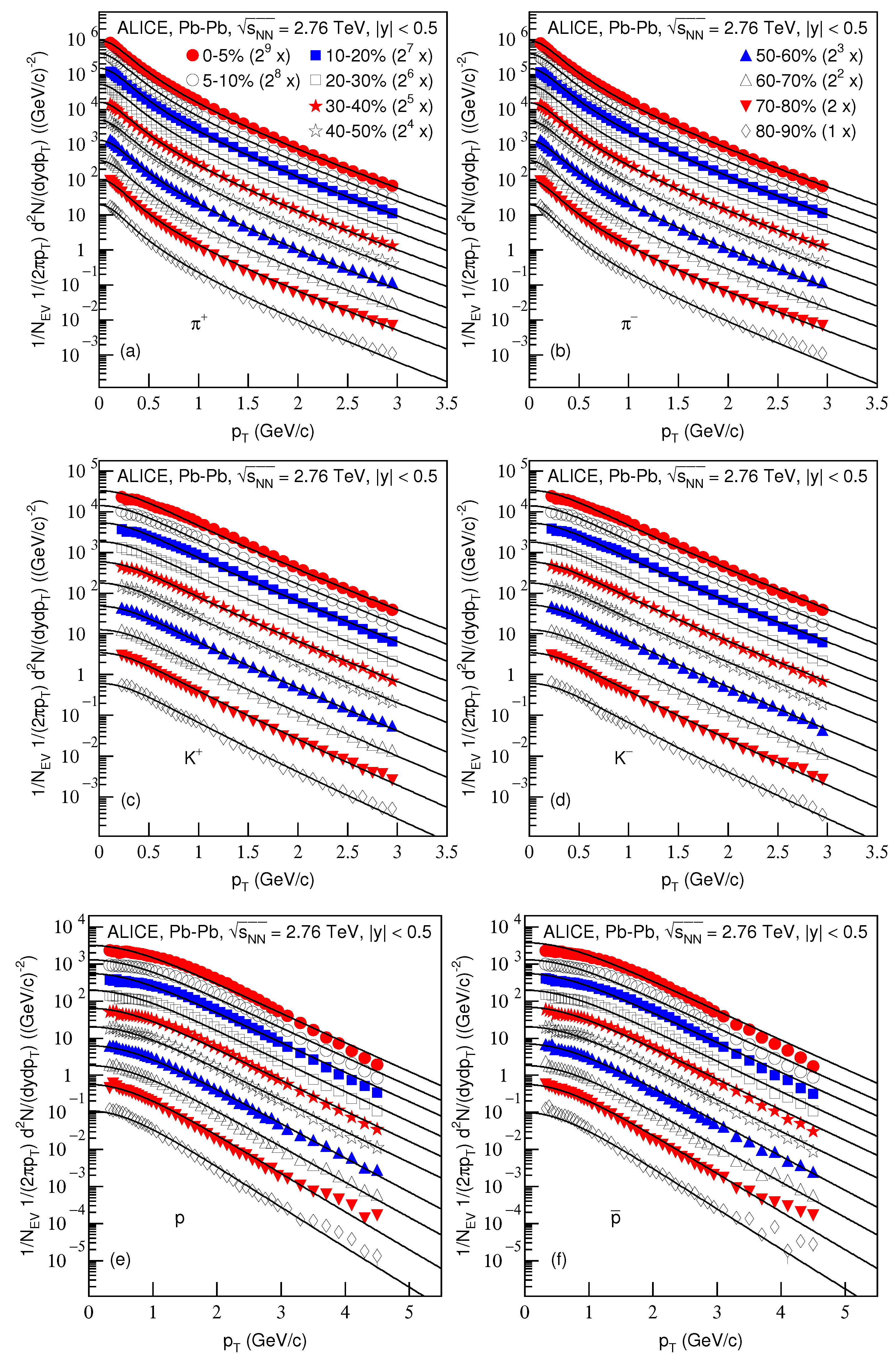
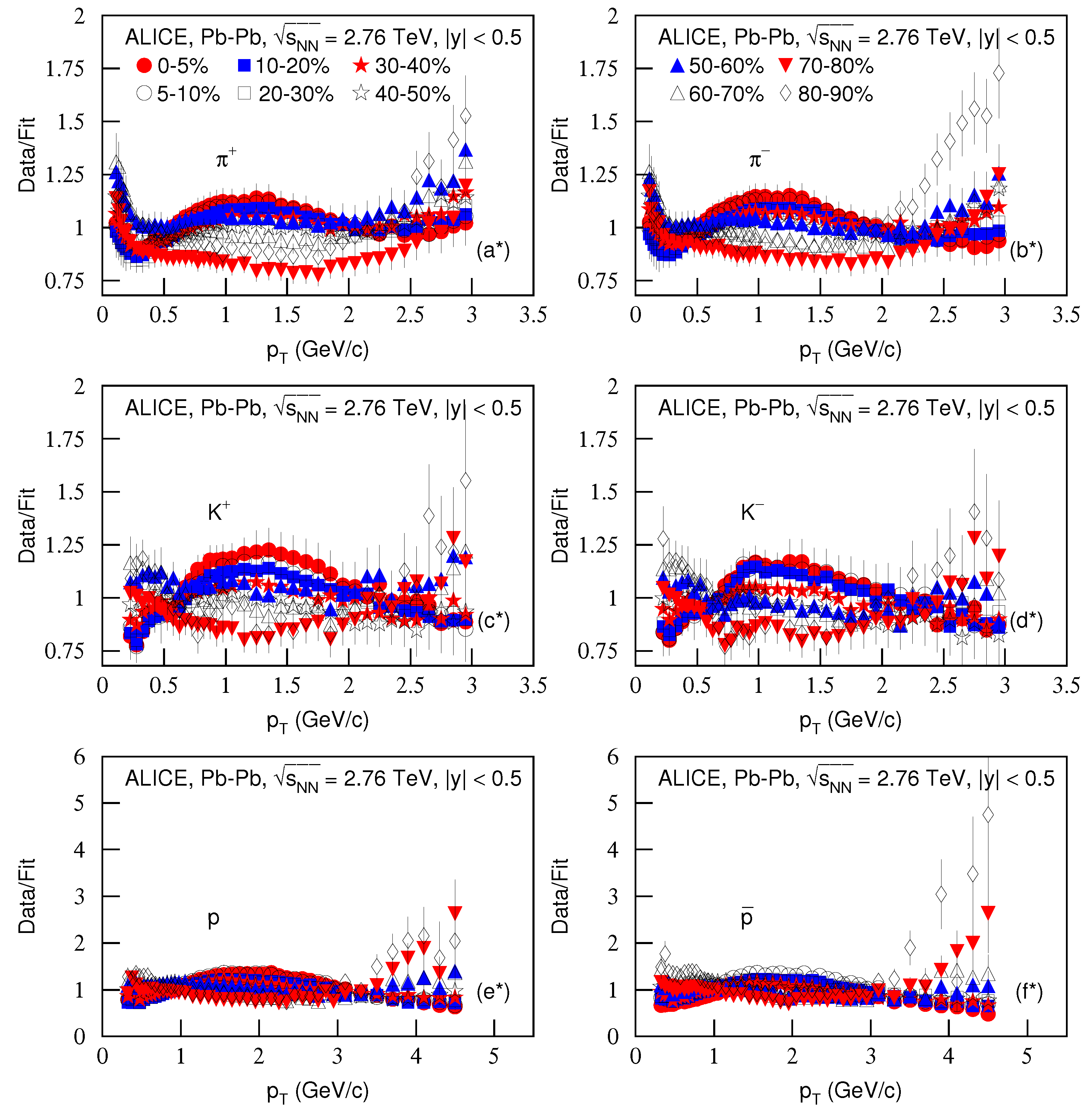
- Abelev, B.; Adam, J.; Adamová, D.; Adare, A.M.; Aggarwal, M.M.; Rinella, G.A.; Agnello, M.; Agocs, A.G.; Agostinelli, A.; Ahammed, Z.; et al. Centrality dependence of π, K, and p in Pb-Pb collisions at TeV. Phys. Rev. C 2013, 88, 044910. [Google Scholar] [CrossRef]
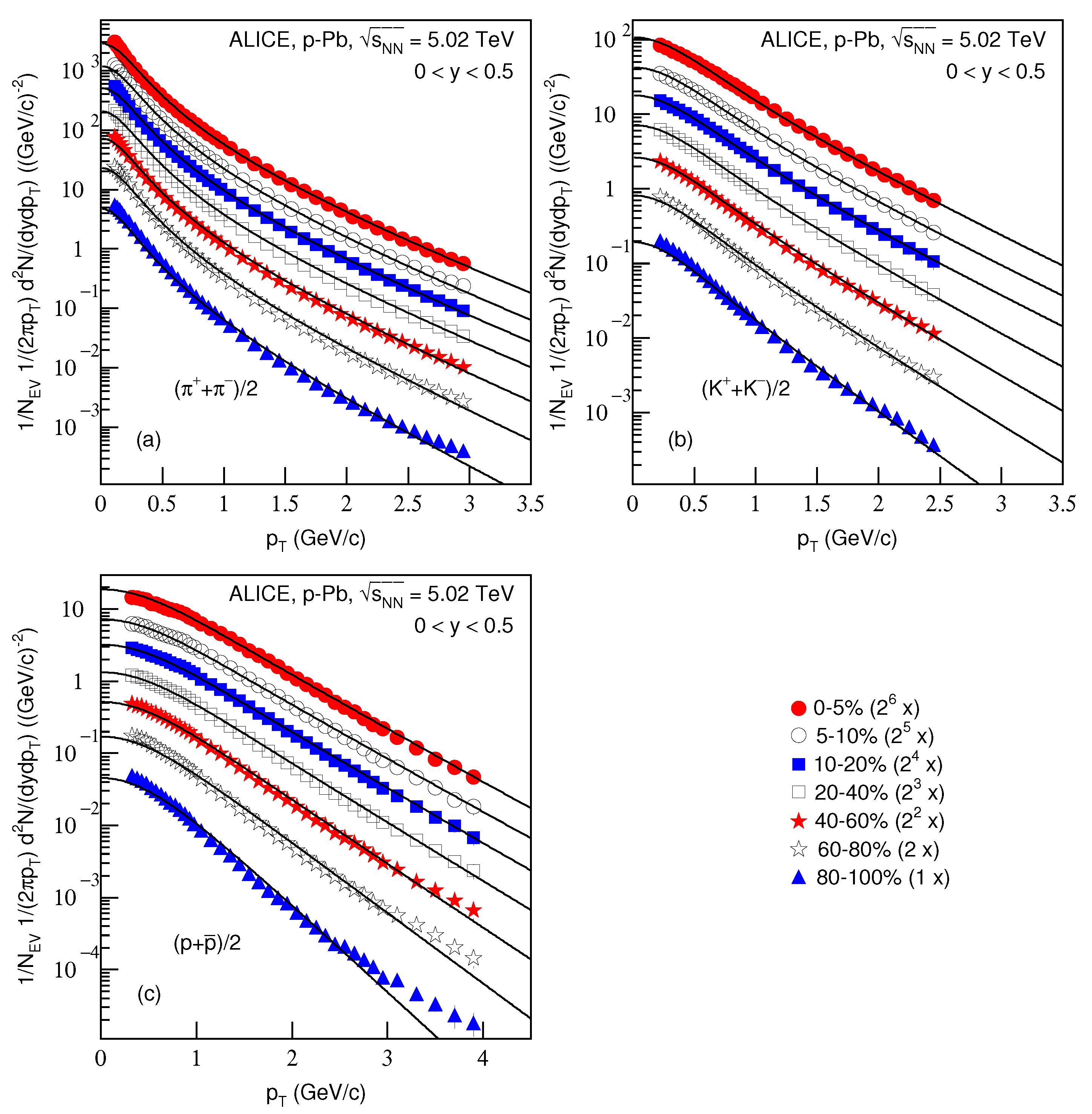
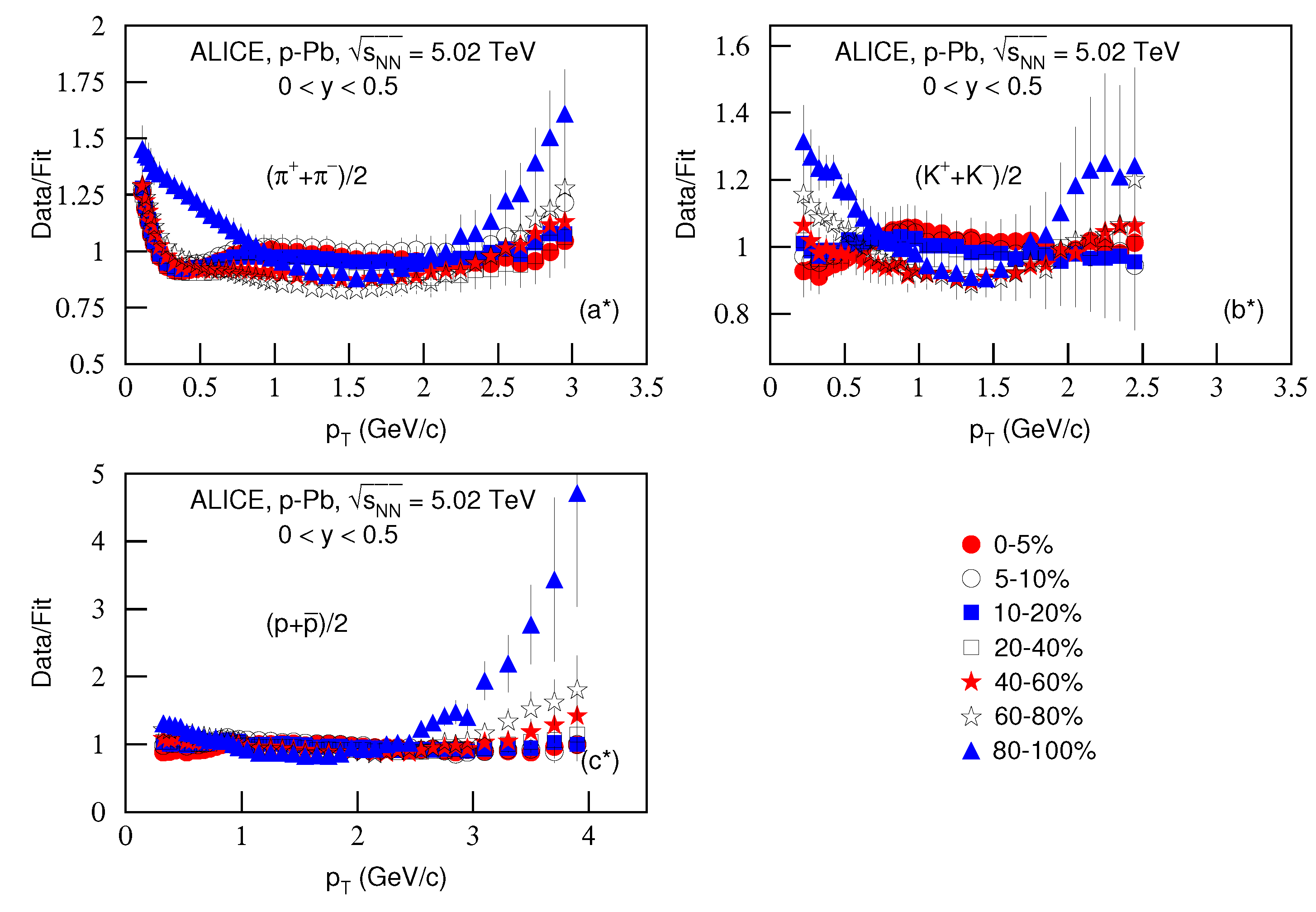
- Abelev, B.; Adam, J.; Adamová, D.; Adare, A.M.; Aggarwal, M.M.; Aglieri Rinella, G.; Agnello, M.; Agocs, A.G.; Agostinelli, A.; Ahammed, Z.; et al. Multiplicity dependence of pion, kaon, proton and lambda production in p-Pb collisions at TeV. Phys. Lett. B 2014, 728, 25–38. [Google Scholar] [CrossRef]
- Ragoni, S.; for the ALICE Collaboration. Production of pions, kaons and protons in Xe-Xe collisions at TeV. arXiv 2018, arXiv:809.01086. [Google Scholar]
- Adam, J.; Adamová, D.; Aggarwal, M.M.; Aglieri Rinella, G.; Agnello, M.; Agrawal, N.; Ahammed, Z.; Ahmad, S.; Ahn, S.; Ahn, S.U.; et al. Multiplicity dependence of charged pion, kaon, and (anti)proton production at large transverse momentum in p-Pb collisions at TeV. Phys. Lett. B 2016, 760, 720. [Google Scholar] [CrossRef]
- Chatrchyan, S.; Khachatryan, V.; Sirunyan, A.M.; Tumasyan, A.; Adam, W.; Aguilo, E.; Bergauer, T.; Dragicevic, M.; Erö, J.; Fabjan, C.; et al. Study of the inclusive production of charged pions, kaons, and protons in pp collisions at = 0.9, 2.76, and 7 TeV. Eur. Phys. J. C 2012, 72, 2164. [Google Scholar] [CrossRef]
- Sirunyan, A.M.; Tumasyan, A.; Adam, W.; Asilar, E.; Bergauer, T.; Brandstetter, J.; Brondolin, E.; Dragicevic, M.; Erö, J.; Flechl, M.; et al. Measurement of charged pion, kaon, and proton production in proton-proton collisions at TeV. Phys. Rev. D 2017, 96, 112003. [Google Scholar] [CrossRef]
- Tomášik, B.; Wiedemann, U.A.; Heinz, U.W. Reconstructing the freeze-out state in Pb+Pb collisions at 158 AGeV/c. Acta Phys. Hung. A 2003, 17, 105–143. [Google Scholar] [CrossRef]
- Ray, R.L.; Jentsch, A. Phenomenological models of two-particle correlation distributions on transverse momentum in relativistic heavy-ion collisions. Phys. Rev. C 2019, 99, 024911. [Google Scholar] [CrossRef]
- Schnedermann, E.; Heinz, U. Relativistic hydrodynamics in a global fashion. Phys. Rev. C 1993, 47, 1738. [Google Scholar] [CrossRef]
- Kumar, L. for the STAR Collaboration. Systematics of kinetic freeze-out properties in high energy collisions from STAR. Nucl. Phys. A 2014, 931, 1114. [Google Scholar] [CrossRef]
- Thakur, D.; Tripathy, S.; Garg, P.; Sahoo, R.; Cleymans, J. Indication of a differential freeze-out in proton-proton and heavy-ion collisions at RHIC and LHC energies. Adv. High Energy Phys. 2016, 2016, 4149352. [Google Scholar] [CrossRef]
- Lao, H.L.; Liu, F.H.; Lacey, R.A. Extracting kinetic freeze-out temperature and radial flow velocity from an improved Tsallis distribution. Eur. Phys. J. A 2017, 53, 44. [Google Scholar] [CrossRef]
- Lao, H.L.; Liu, F.H.; Li, B.C.; Duan, M.Y. Kinetic freeze-out temperatures in central and peripheral collisions: Which one is larger? Nucl. Sci. Tech. 2018, 29, 82. [Google Scholar] [CrossRef]
- Thakur, D.; Tripathy, S.; Garg, P.; Sahoo, R.; Cleymans, J. Indication of differential kinetic freeze-out at RHIC and LHC energies. Acta Phys. Polon. Supp. 2016, 9, 329–332. [Google Scholar] [CrossRef]
- Sahoo, R. Possible formation of QGP-droplets in proton-proton collisions at the CERN Large Hadron Collider. AAPPS Bull. 2019, 29, 16–21. [Google Scholar]


| Figure | Centrality | Particle | (GeV) | (c) | (fm/c) | /dof | (fm/c) |
|---|---|---|---|---|---|---|---|
| 1a | 0–5% | 203,000.0 ± 20,900.0 | 50.7/38 | ||||
| Pb–Pb | 5–10% | 170,000.0 ± 18,000.0 | 48.8/38 | ||||
| 10–20% | 130,000.0 ± 14,000.0 | 44.3/38 | |||||
| 20–30% | 90,000.0 ± 9900.0 | 50.5/38 | |||||
| 30–40% | 56,000.0 ± 6100.0 | 28.4/38 | |||||
| 40–50% | 34,000.0 ± 3700.0 | 19.5/38 | |||||
| 50–60% | 19,000.0 ± 2200.0 | 44.1/38 | |||||
| 60–70% | 10,000.0 ± 1200.0 | 43.5/38 | |||||
| 70–80% | 335.9/38 | ||||||
| 80–90% | 97.6/38 | ||||||
| 1b | 0–5% | 198,000.0 ± 20,600.0 | 68.6/38 | ||||
| Pb–Pb | 5–10% | 165,000.0 ± 17,000.0 | 58.2/38 | ||||
| 10–20% | 128,000.0 ± 13,000.0 | 43.7/38 | |||||
| 20–30% | 85,000.0 ± 9500.0 | 32.6/38 | |||||
| 30–40% | 54,000.0 ± 5900.0 | 22.2/38 | |||||
| 40–50% | 33,000.0 ± 3700.0 | 15.2/38 | |||||
| 50–60% | 19,000.0 ± 2200.0 | 25.0/38 | |||||
| 60–70% | 10,000.0 ± 1200.0 | 45.0/38 | |||||
| 70–80% | 184.1/38 | ||||||
| 80–90% | 98.3/38 | ||||||
| 1c | 0–5% | 87.9/33 | |||||
| Pb–Pb | 5–10% | 68.7/33 | |||||
| 10–20% | 58.2/33 | ||||||
| 20–30% | 40.2/33 | ||||||
| 30–40% | 18.5/33 | ||||||
| 40–50% | 14.9/33 | ||||||
| 50–60% | 24.9/33 | ||||||
| 60–70% | 20.8/33 | ||||||
| 70–80% | 92.5/33 | ||||||
| 80–90% | 50.3/33 | ||||||
| 1d | 0–5% | 10,100.0 ± 1100.0 | 58.3/33 | ||||
| Pb–Pb | 5–10% | 55.3/33 | |||||
| 10–20% | 46.7/33 | ||||||
| 20–30% | 25.3/33 | ||||||
| 30–40% | 13.3/33 | ||||||
| 40–50% | 14.8/33 | ||||||
| 50–60% | 13.4/33 | ||||||
| 60–70% | 25.8/33 | ||||||
| 70–80% | 95.0/33 | ||||||
| 80–90% | 66.7/33 | ||||||
| 1e | 0–5% | p | 243.0/39 | ||||
| Pb–Pb | 5–10% | 238.1/39 | |||||
| 10–20% | 160.8/39 | ||||||
| 20–30% | 120.9/39 | ||||||
| 30–40% | 87.9/39 | ||||||
| 40–50% | 68.1/39 | ||||||
| 50–60% | 53.4/39 | ||||||
| 60–70% | 101.5/39 | ||||||
| 70–80% | 222.7/39 | ||||||
| 80–90% | 95.6/39 | ||||||
| 1f | 0–5% | 174.0/39 | |||||
| Pb–Pb | 5–10% | 197.0/39 | |||||
| 10–20% | 143.6/39 | ||||||
| 20–30% | 106.2/39 | ||||||
| 30–40% | 81.8/39 | ||||||
| 40–50% | 101/39 | ||||||
| 50–60% | 47.0/39 | ||||||
| 60–70% | 92.1/39 | ||||||
| 70–80% | 144.1/39 | ||||||
| 80–90% | 115.1/39 | ||||||
| 3a | 0–5% | ( | 163,500.0 ± 22,250.0 | 78.1/38 | |||
| p–Pb | 5–10% | 143,500.0 ± 19,680.0 | 62.3/38 | ||||
| 10–20% | 123,500.0 ± 16,550.0 | 82.3/38 | |||||
| 20–40% | 103,500.0 ± 15,500.0 | 170.6/38 | |||||
| 40–60% | 72,000.0 ± 10,650.0 | 183.1/38 | |||||
| 60–80% | 47,000.0 ± 6200.0 | 277.2/38 | |||||
| 80–100% | 22,000.0 ± 2305.0 | 516.5/38 | |||||
| 3b | 0–5% | ( | 12,000.0 ± 1805.0 | 15.8/28 | |||
| p–Pb | 5–10% | 5.7/28 | |||||
| 10–20% | 2.7/28 | ||||||
| 20–40% | 7.4/28 | ||||||
| 40–60% | 35.0/28 | ||||||
| 60–80% | 50.0/28 | ||||||
| 80–100% | 125.9/28 | ||||||
| 3c | 0–5% | ( | 41.8/36 | ||||
| p–Pb | 5–10% | 26.7/36 | |||||
| 10–20% | 21.3/36 | ||||||
| 20–40% | 37.6/36 | ||||||
| 40–60% | 57.7/36 | ||||||
| 60–80% | 116.1/36 | ||||||
| 80–100% | 192.5/36 | ||||||
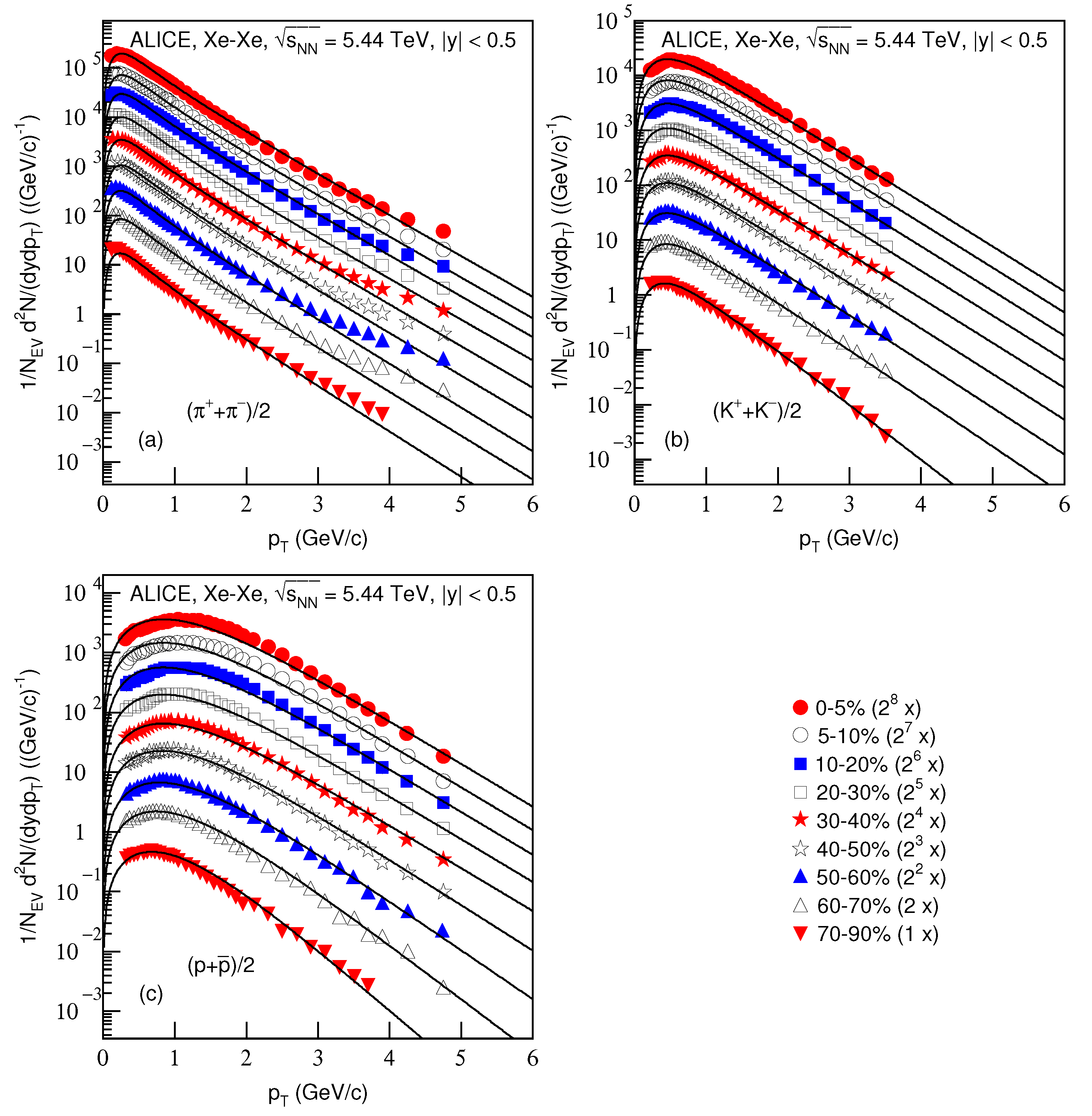
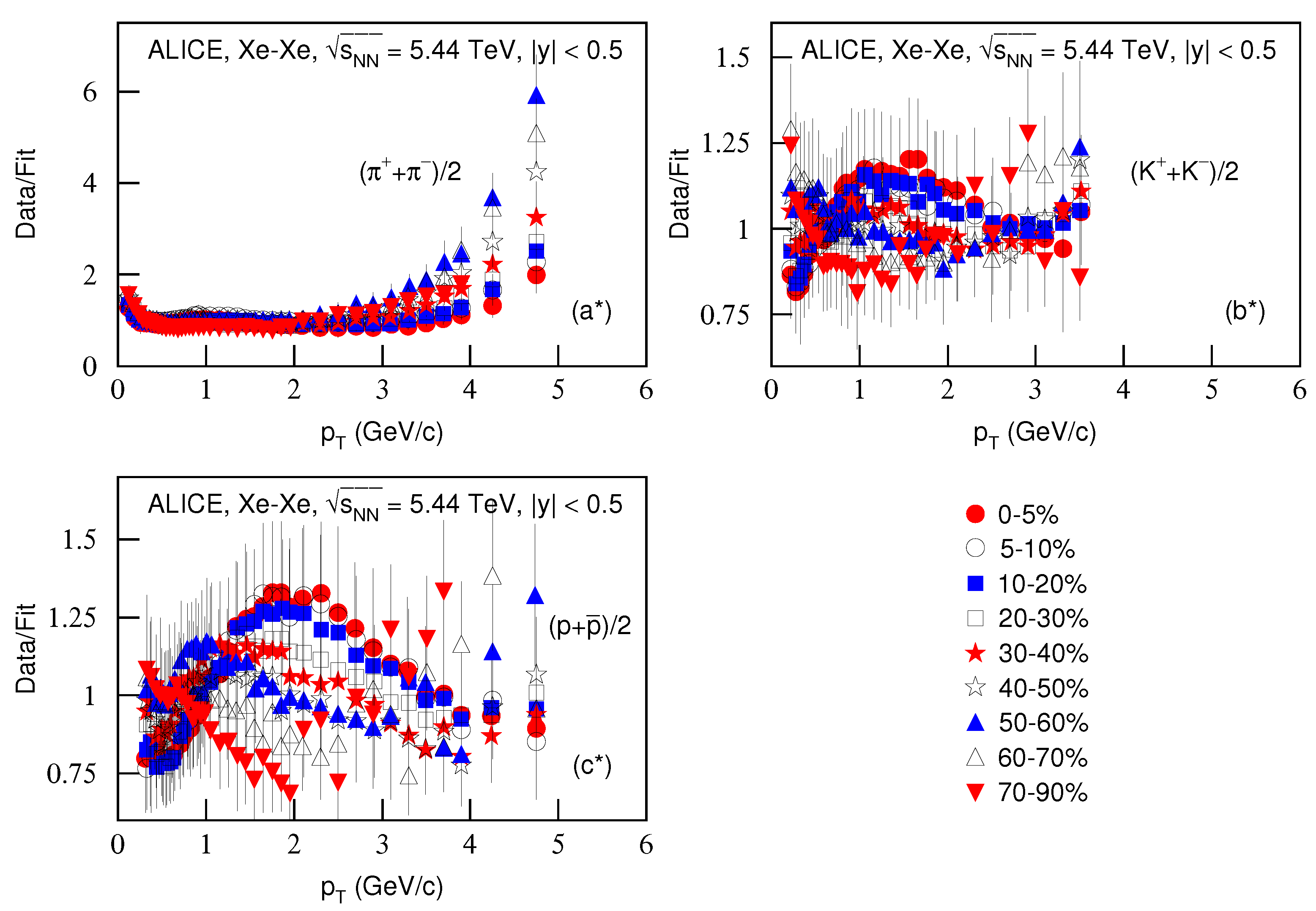
| 5a | 0–5% | ( | 67,892.5 ± 8920.0 | 19.5/38 | |||
| Xe–Xe | 5–10% | 49,892.5 ± 6044.0 | 19.2/38 | ||||
| 10–20% | 41,392.5 ± 4678.0 | 23.9/38 | |||||
| 20–30% | 27,892.5 ± 3462.0 | 40.6/38 | |||||
| 30–40% | 20,392.5 ± 2569.0 | 42.4/38 | |||||
| 40–50% | 13,142.5 ± 1581.0 | 53.0/38 | |||||
| 50–60% | 109.1/38 | ||||||
| 60–70% | 79.8/38 | ||||||
| 70–90% | 69.3/38 | ||||||
| 5b | 0–5% | ( | 18.1/30 | ||||
| Xe–Xe | 5–10% | 13.5/30 | |||||
| 10–20% | 10.5/30 | ||||||
| 20–30% | 5.4/30 | ||||||
| 30–40% | 3.4/30 | ||||||
| 40–50% | 5.1/30 | ||||||
| 50–60% | 5.4/30 | ||||||
| 60–70% | 13.8/30 | ||||||
| 70–90% | 20.2/30 | ||||||
| 5c | 0–5% | ( | 37.9/32 | ||||
| Xe–Xe | 5–10% | 37.6/32 | |||||
| 10–20% | 30.6/32 | ||||||
| 20–30% | 19.4/32 | ||||||
| 30–40% | 14.1/32 | ||||||
| 40–50% | 11.0/32 | ||||||
| 50–60% | 13.8/32 | ||||||
| 60–70% | 17.5/32 | ||||||
| 70–90% | 41.7/29 |
| Figure | Energy (TeV) | Particle | (GeV) | (c) | (fm/c) | /dof | (fm/c) |
|---|---|---|---|---|---|---|---|
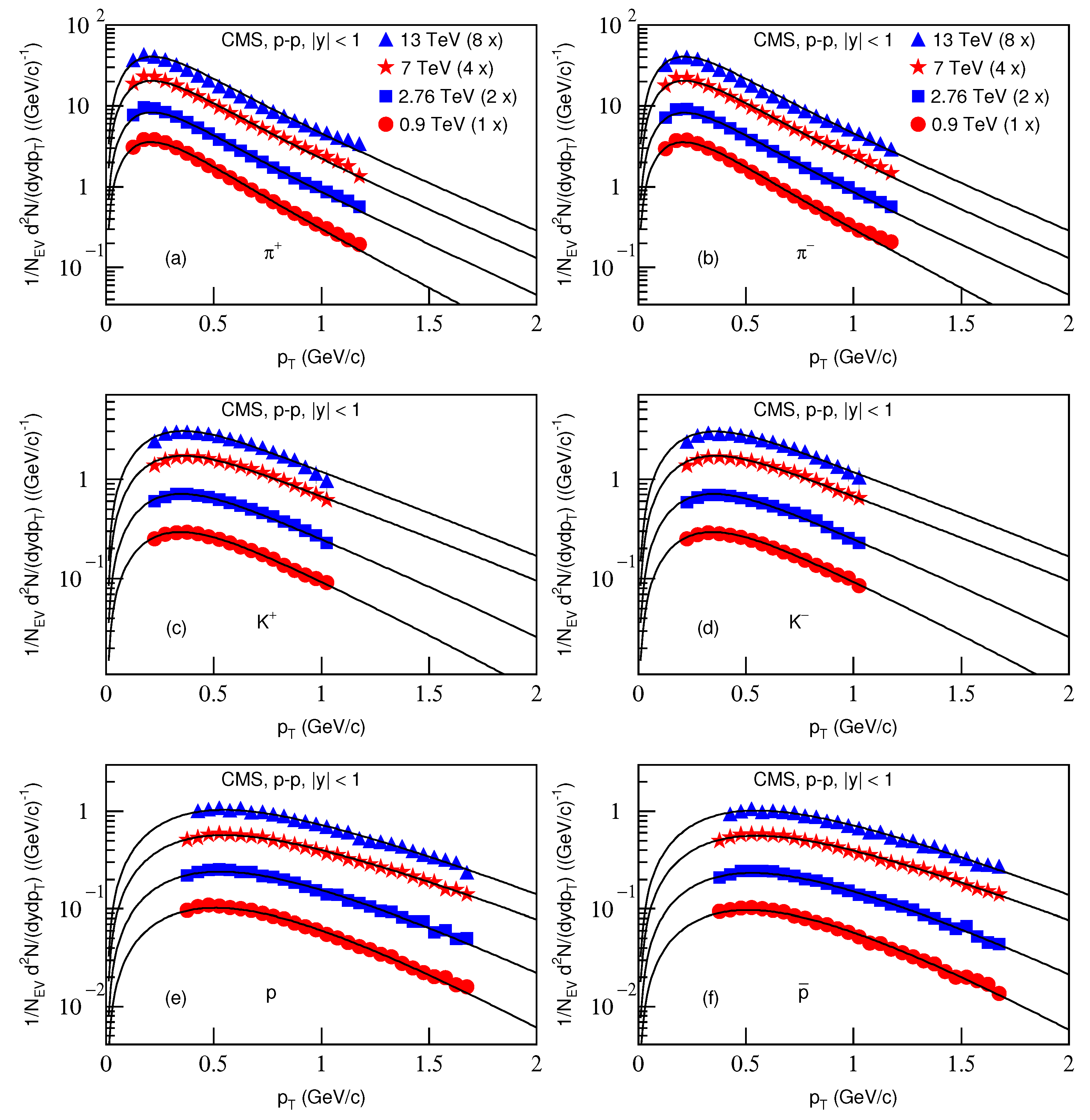
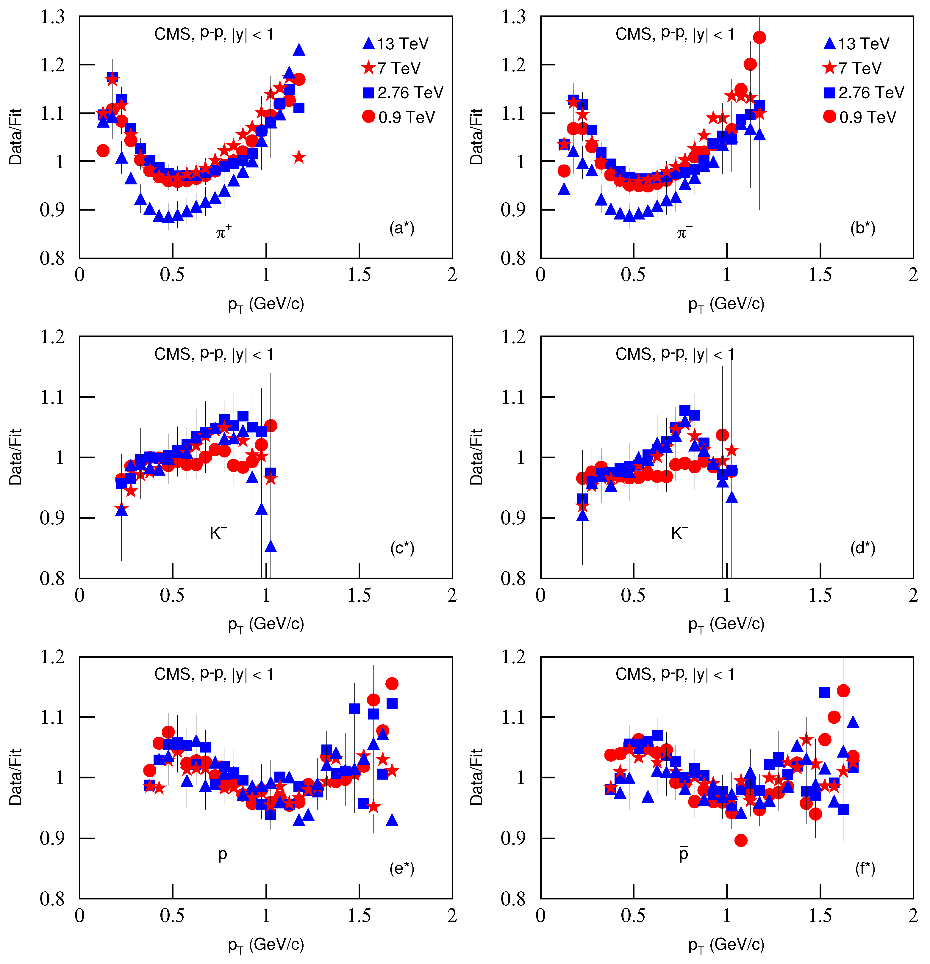
| 7a | 0.9 | 10,785.0 ± 1110.0 | 84.9/19 | ||||
| p–p | 2.76 | 12,785.0 ± 1300.0 | 105.3/19 | ||||
| 7 | 15,785.0 ± 1590.0 | 120.3/19 | |||||
| 13 | 15,785.0 ±1585.0 | 132.7/19 | |||||
| 7b | 0.9 | 10,725.0 ± 1110.0 | 117.9/19 | ||||
| p–p | 2.76 | 12,705.0 ± 1300.0 | 85.7/19 | ||||
| 7 | 15,815.0 ± 1590.0 | 116.0/19 | |||||
| 13 | 15,785.0 ± 1585.0 | 113.4/19 | |||||
| 7c | 0.9 | 3.3/14 | |||||
| p–p | 2.76 | 21.2/14 | |||||
| 7 | 20.2/14 | ||||||
| 13 | 5.2/14 | ||||||
| 7d | 0.9 | 16.7/14 | |||||
| p–p | 2.76 | 23.3/14 | |||||
| 7 | 22.9/14 | ||||||
| 13 | 6.5/14 | ||||||
| 7e | 0.9 | p | 37.9/24 | ||||
| p–p | 2.76 | 48.9/24 | |||||
| 7 | 21.2/24 | ||||||
| 13 | 15.3/23 | ||||||
| 7f | 0.9 | 66.8/24 | |||||
| p–p | 2.76 | 37.9/24 | |||||
| 7 | 23.4/24 | ||||||
| 13 | 11.9/23 | ||||||
| 9 | 5.02 | ( | 11,242.5 ± 1055.0 | 187.6/28 | |||
| ( | 13.7/23 | ||||||
| ( | 23.5/21 |
| Figure | Centrality | b (fm) | (fm/c) | (fm/c) |
|---|---|---|---|---|
| 14a | 0–5% | 2.117 | ||
| Pb–Pb | 5–10% | 3.867 | ||
| 10–20% | 5.468 | |||
| 20–30% | 7.083 | |||
| 30–40% | 8.391 | |||
| 40–50% | 9.514 | |||
| 50–60% | 10.521 | |||
| 60–70% | 11.443 | |||
| 70–80% | 12.293 | |||
| 80–90% | 13.087 | |||
| 14a | 0–5% | 1.237 | ||
| p–Pb | 5–10% | 2.258 | ||
| 10–20% | 3.196 | |||
| 20–40% | 4.520 | |||
| 40–60% | 5.853 | |||
| 60–80% | 6.935 | |||
| 80–100% | 7.866 | |||
| 14a | 0–5% | 1.817 | ||
| Xe–Xe | 5–10% | 3.320 | ||
| 10–20% | 4.698 | |||
| 20–30% | 6.086 | |||
| 30–40% | 7.209 | |||
| 40–50% | 8.179 | |||
| 50–60% | 9.042 | |||
| 60–70% | 9.829 | |||
| 70–90% | 10.900 |
| Figure | Energy (TeV) | (fm/c) | (fm/c) |
|---|---|---|---|
| 14b | 0.9 | ||
| p–p | 2.76 | ||
| 5.02 | |||
| 7 | |||
| 13 | |||
| Pb–Pb | 2.76 | ||
| p–Pb | 5.02 | ||
| Xe–Xe | 5.44 |
Publisher’s Note: MDPI stays neutral with regard to jurisdictional claims in published maps and institutional affiliations. |
© 2021 by the authors. Licensee MDPI, Basel, Switzerland. This article is an open access article distributed under the terms and conditions of the Creative Commons Attribution (CC BY) license (https://creativecommons.org/licenses/by/4.0/).
Share and Cite
Lao, H.-L.; Liu, F.-H.; Ma, B.-Q. Analyzing Transverse Momentum Spectra of Pions, Kaons and Protons in p–p, p–A and A–A Collisions via the Blast-Wave Model with Fluctuations. Entropy 2021, 23, 803. https://doi.org/10.3390/e23070803
Lao H-L, Liu F-H, Ma B-Q. Analyzing Transverse Momentum Spectra of Pions, Kaons and Protons in p–p, p–A and A–A Collisions via the Blast-Wave Model with Fluctuations. Entropy. 2021; 23(7):803. https://doi.org/10.3390/e23070803
Chicago/Turabian StyleLao, Hai-Ling, Fu-Hu Liu, and Bo-Qiang Ma. 2021. "Analyzing Transverse Momentum Spectra of Pions, Kaons and Protons in p–p, p–A and A–A Collisions via the Blast-Wave Model with Fluctuations" Entropy 23, no. 7: 803. https://doi.org/10.3390/e23070803
APA StyleLao, H.-L., Liu, F.-H., & Ma, B.-Q. (2021). Analyzing Transverse Momentum Spectra of Pions, Kaons and Protons in p–p, p–A and A–A Collisions via the Blast-Wave Model with Fluctuations. Entropy, 23(7), 803. https://doi.org/10.3390/e23070803