Abstract
The classical Schalkwijk–Kailath (SK) scheme for the point-to-point white Gaussian channel with noiseless feedback plays an important role in information theory due to the fact that it is capacity-achieving and the complexity of its encoding–decoding procedure is extremely low. In recent years, it has been shown that an extended SK feedback scheme also achieves the capacity region of the two-user Gaussian multiple-access channel with noiseless feedback (GMAC-NF), where two independent messages are, respectively, encoded by two intended transmitters. However, for the two-user GMAC-NF with degraded message sets (one common message for both users and one private message for an intended user), the capacity-achieving feedback scheme remains open. In this paper, we propose a novel two-step SK-type feedback scheme for the two-user GMAC-NF with degraded message sets and show that this scheme is capacity-achieving.
1. Introduction
Shannon showed that feedback does not increase the capacity of the discrete memoryless channel (DMC) [1]. Later, Schalkwijk and Kailath [2] proposed a feedback coding scheme called the SK scheme and showed that this scheme is capacity-achieving and greatly improves the encoding–decoding performance of the point-to-point white Gaussian channel. According to the landmark paper [2], Ozarow [3] extended the classic SK scheme [2] to a multiple-access situation; namely, the two-user Gaussian multiple-access channel (GMAC) with noiseless feedback (GMAC-NF), where two independent messages are, respectively, encoded by two intended transmitters. Similar to [2], Ozarow showed that this extended scheme is also capacity-achieving, i.e., achieving the capacity region of the two-user GMAC-NF. Parallel work of [3] involves extending the classic SK scheme [2] to a broadcast situation; namely, the Gaussian broadcast channel with noiseless feedback (GBC-NF). Ref. [4] proposed an SK-type feedback scheme for the GBC-NF, but unfortunately this scheme is not capacity-achieving. Other applications of SK schemes include the following:
- Weissman and Merhav [5] proposed an SK-type feedback scheme for the dirty paper channel with noiseless feedback and showed that this scheme is capacity-achieving. Subsequently, Rosenzweig [6] extended the SK-type scheme of [5] to multiple-access and broadcast situations.
- Kim extended the SK scheme to colored (non-white) Gaussian channels with noiseless feedback [7,8] and showed that these extended schemes are also capacity-achieving for some special cases.
- Bross [9] extended the SK-type scheme to the Gaussian relay channel with noiseless feedback and showed that the proposed scheme is better than the ones already existing in the literature.
- Ben-Yishai and Shayevitz [10] studied the SK-type scheme for the white Gaussian channel with noisy feedback and showed that a variation of the SK scheme achieves a rate that tends to be the capacity for some special cases.
In this paper, we revisit the two-user GMAC-NF by considering the case that one common message for both users and one private message for an intended user are transmitted through the channel (see Figure 1), which is also called the two-user GMAC with degraded message sets and noiseless feedback (GMAC-DMS-NF). Here, note that the two-user GMAC with degraded message sets is especially useful when considering partial cooperation between the encoders of the GMAC. Although it has already been shown that feedback does not increase the capacity region of the two-user GMAC-DMS-NF, the capacity-achieving SK-type feedback scheme of this model remains open. In this paper, a novel SK-type feedback scheme is proposed for the model of Figure 1 and it is proven to be capacity-achieving.
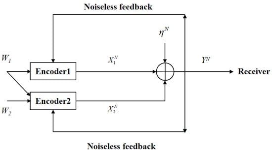
Figure 1.
The two-user GMAC with degraded message sets and noiseless feedback.
2. Preliminary
In this section, we introduce the SK schemes for the point-to-point white Gaussian channel with feedback and the two-user GMAC-NF.
Basic notation: A random variable (RV) is denoted with an upper case letter (e.g., X), its value is denoted with an lower case letter (e.g., x), the finite alphabet of the RV is denoted with calligraphic letter (e.g., ), and the probability distribution of an event is denoted with . A random vector and its value are denoted by a similar convention. For example, represents an N-dimensional random vector , and represents a vector value in (the N-th Cartesian power of the finite alphabet ). In addition, define and . Throughout this paper, the base of the log function is 2.
2.1. The SK Scheme for the Point-to-Point White Gaussian Channel with Feedback
For the white Gaussian channel with feedback (see Figure 2), at time instant i (), the channel input and output are given by
where is the channel output, is the channel input, and is the i.i.d white Gaussian noise across the time index i. The message W is uniformly chosen from the set , and the i-th time channel input is a function of the message W and the feedback , namely,
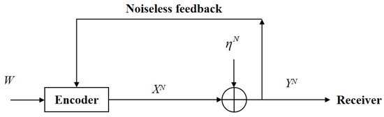
Figure 2.
The point-to-point white Gaussian channel with feedback.
The receiver obtains an estimation , where is the receiver’s decoding function, and the average decoding error probability is given by
For a given positive rate R, if for arbitrarily small and sufficiently large N, there exists a channel encoder–decoder such that
we say that R is achievable. The channel capacity is the maximum over all achievable rates. Denote the capacity of the white Gaussian channel with feedback by . Since feedback does not increase , it is easy to see that
where is the capacity of the white Gaussian channel (the same model without feedback).
In [2], it has been shown that the classical SK scheme achieves , and it consists of the following two properties:
- At time 1, the channel input is a deterministic function of the real transmitted message.
- From time 2 to N, the channel input is the linear combination of previous channel noise.
The details of the SK scheme are described below.
Let be the message set of W, divide the interval into equally spaced sub-intervals, and each sub-interval center corresponds to a value in W. The center of the sub-interval with respect to (w.r.t.) W is denoted by , where the variance of approximately equals .
At time 1, the transmitter transmits
The receiver receives , and obtains an estimation of by computing
where , and .
At time k (), the transmitter sends
where .
In [2], it has been shown that the decoding error of the above coding scheme is upper-bounded by
where is the tail of the unit Gaussian distribution evaluated at x, and
as .
2.2. The Two-User GMAC with Degraded Message Sets
The channel model consisting of two inputs, one output, and the Gaussian channel noise is called GMAC. On the basis of GMAC, if message is known by encoder 1 and encoder 2, message 2 is only known by encoder 2, and this model is called GMAC-DMS.
The GMAC with degraded message sets is shown in Figure 3. At time i (), the channel inputs and output are given by
where , are the channel inputs, respectively, subject to average power constraints and , namely, , , is the channel output, is i.i.d. Gaussian noise across i. The message is uniformly drawn in the set . The input is a function of the message , and the input is a function of both messages and . After receiving the channel output, the receiver computes for decoding, where is the receiver’s decoding function. The average decoding error probability is defined as
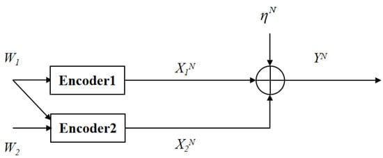
Figure 3.
The GMAC with degraded message sets.
A rate pair is said to be achievable if, for any and sufficiently large N, there exist channel encoders and decoder such that
The capacity region of the GMAC-DMS is noted as , which is composed of all such achievable rate pairs.
Theorem 1.
The capacity regionis given by
Proof.
Achievability proof of : From [11], the capacity region of the discrete memoryless multiple-access channel with degraded message sets is given by
for some joint distribution . Then, substituting , and (15) into (19), defining
and following the idea of the encoding–decoding scheme of [11], the achievability of is proved.
Converse proof of : The converse proof of follows the converse part of GMAC with feedback [3] (see the converse proof of the bounds on and ), and hence we omit the details here. The proof of Theorem 1 is completed. □
3. Model Formulation and the Main Results
In this section, we will first give a formal definition of the two-user GMAC-DMS-NF, then we will give the main results of this paper.
3.1. The Two-User GMAC-DMS-NF
The two-user GMAC-DMS-NF is shown in Figure 1. At time i (), the channel inputs and output are given by
where , are the channel inputs, respectively, subject to average power constraints and , namely, , , is the channel output, is the i.i.d. Gaussian noise across i. The message is uniformly drawn in the set . At time i, the input is a function of the common message and the feedback , and the input is a function of the common message , the private message , and the feedback . After receiving the channel output, the receiver generates an estimation pair , where is the receiver’s decoding function. This model’s average decoding error probability equals
The capacity region of the two-user GMAC-DMS-NF is noted as , and it is characterized in the following Theorem 2.
Theorem 2.
, where is given in Theorem 1.
Proof.
From the converse proof of the bounds on and in [3], we conclude that
However, since the non-feedback model is a special case of the feedback model, thus we have
The proof of Theorem 2 is completed. □
3.2. A Capacity-Achieving SK-Type Scheme for the Two-User GMAC-DMS-NF
In this subsection, we propose a two-step SK-type scheme for the two-user GMAC-DMS-NF, and show that this scheme is capacity-achieving, i.e., achieving . This new scheme is briefly described in the following Figure 4.
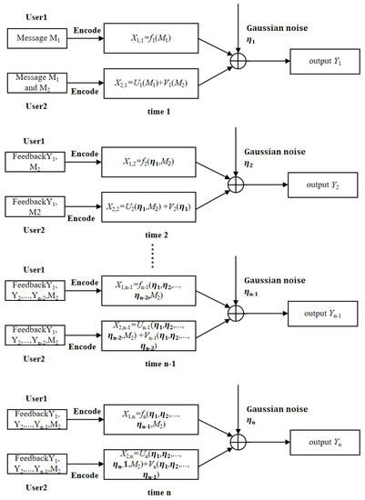
Figure 4.
A two-step SK-type scheme for the two-user GMAC-DMS-NF.
The common message is encoded by both transmitters, and the private message is only available by Transmitter 2. Transmitter 1 uses power to encode and the feedback as . Transmitter 2 uses power to encode and the feedback as , and power to encode and the feedback as , where . Here note that since is known by Transmitter 2, the codewords and can be subtracted when applying the SK scheme to , i.e., for the SK scheme of , the equivalent channel model has input , output , and channel noise .
In addition, since is known by both transmitters and is only available at Transmitter 2, for the SK scheme of , the equivalent channel model has inputs and , output , and channel noise , which is non-white Gaussian noise since is not i.i.d. generated. Furthermore, we observe that
where , is Gaussian-distributed with zero mean and variance ,
where
and . Hence for the SK scheme of , the input of the equivalent channel model can be viewed as , where . Define
Then we have , which leads to
where . The encoding and decoding procedure of Figure 4 is described below.
3.2.1. Encoding Procedure for the Two-Step SK-Type Scheme
Define and divide the interval into equally spaced sub-intervals. The center of each sub-interval is mapped to a message value in (). Let be the center of the sub-interval w.r.t. the message (the variance of approximately equals ).
At time 1, Transmitter 2 sends
Transmitter 1 and Transmitter 2, respectively, send , such that
The receiver obtains and sends back to Transmitter 2. Subtracting and from and letting , Transmitter 2 computes
and defines . Since , Transmitter 1 computes
and defines
At time 2, Transmitter 2 sends
In the meantime, Transmitter 1 and Transmitter 2, respectively, send and such that
At time , once it has received , Transmitter 2 computes
and sends
where . In the meantime, Transmitters 1 and 2, respectively, send and such that
where
and .
3.2.2. Decoding Procedure for the Two-Step SK-Type Scheme
The decoding procedure for the receiver consists of two steps. First, from (8), we see that at time , the receiver’s estimation of is given by
where and
Second, after decoding and the corresponding codewords and for all , the receiver subtracts and from , and obtains . At time , the receiver computes of by
where and
The receiver’s decoding error probability for is upper-bounded by
From the classical SK scheme [2] (also introduced in Section 2.1), we know that the decoding error probability of tends to 0 as if
and hence we omit the derivation here. The decoding error probability is upper-bounded by the following Lemma 1.
Lemma 1.
as if is satisfied.
Proof.
See Appendix A. □
From (46) and Lemma 1, we can conclude that if , the decoding error probability of the receiver tends to 0 as . In other words, the rate pair is achievable for all , which indicates that all rate pairs in are achievable. Hence this two-step SK-type feedback scheme achieves the capacity region of the two-user GMAC-DMS-NF.
4. Conclusions
In this paper, we have proposed a capacity-achieving SK-type feedback scheme for the two-user GMAC-DMS-NF, which remains open in the literature. The proposed scheme in this paper adopts a two-step encoding–decoding procedure, where the common message is encoded as the codeword and one part of the codeword (namely, ), the private message is encoded as the other part of the codeword (namely, ), and the SK scheme is applied to the encoding procedure of both common and private messages. In the decoding procedure, the receiver first decodes the common message by using the SK decoding scheme and viewing as part of the channel noise. Then, after successfully decoding the common message, the receiver subtracts its corresponding codewords and from its received signal , and uses the SK decoding scheme to decode the private message. Here note that the proposed two-step SK-type scheme is not a trivial extension of the already existing feedback scheme [3] for the two-user GMAC, where two independent encoders apply the SK scheme to encode their independent messages. In fact, a simple application of Ozarow’s SK-type scheme [3] cannot achieve the capacity region of the two-user GMAC-DMS-NF, which indicates that it is not an optimal choice for the two-user GMAC-DMS-NF. Possible future work includes the following:
- Capacity-achieving SK-type feedback schemes for the fading GMAC.
- SK-type feedback schemes for the GMAC with noisy feedback.
Author Contributions
H.Y. performed the theoretical work and the experiments, analyzed the data and drafted the work; B.D. designed the work, performed the theoretical work, analyzed the data, interpreted data for the work and revised the work. All authors have read and agreed to the published version of the manuscript.
Funding
This work was supported in part by the National Key R&D Program of China under Grant 2019YFB1803400; in part by the National Natural Science Foundation of China under Grant 62071392; in part by the Open Research Fund of the State Key Laboratory of Integrated Services Networks, Xidian University, under Grant ISN21-12; and in part by the 111 Project No.111-2-14.
Institutional Review Board Statement
Not applicable.
Informed Consent Statement
Not applicable.
Data Availability Statement
The data used in this work are available from the corresponding author upon reasonable request.
Acknowledgments
Authors would like to thank anonymous reviewers for careful reading of the manuscript and providing constructive comments and suggestions, which have helped them to improve the quality of the paper.
Conflicts of Interest
The authors declare no conflict of interest.
Abbreviations
The following abbreviations are used in this manuscript:
| SK | Schalkwijk–Kailath |
| GMAC | Gaussian multiple-access channel |
| GMAC-NF | Gaussian multiple-access channel with noiseless feedback |
| DMC | Discrete memoryless channel |
| GBC-NF | Gaussian broadcast channel with noiseless feedback |
| GMAC-DMS | Two-user GMAC with degraded message sets |
| GMAC-DMS-NF | Two-user GMAC with degraded message sets and noiseless feedback |
Appendix A
Appendix A proves Lemma 1 described in Section 3. First, we determine the channel noise of the equivalent channel model. For the SK scheme of , the equivalent channel model has input , output , and channel noise , where is non-white Gaussian because is generated by the classical SK scheme and it is a combination of previous channel noise. For , define
Note that
where follows from the fact that is independent of since is a function of and is a function of , and follows from (38). Furthermore, from (37) and (38), can be re-written as
where follows from and is independent of , , , and follows from . Substituting (A3) into (A1), we have
Here note that (A6) holds for , and
After determining the noise expression of the equivalent channel model, we still need to determine the decoding error . According to (40), we have
and
where follows from (39), and follows from (A2). Substituting (A8) and (A9) into (40), can be re-written as
From (A10), we see that depends on . Combining (A6) with (A10), we can conclude that
where follows from , and follows from (A6), which indicates that
where follows from . From (A10) and the fact that
it is easy to see that
for all . The final step before we bound is the determination of , which is defined as . Using (A10), we have
where follows from (A2), follows from the definitions
and follows from (A13) that . Since and , (A14) can be re-written as
where follows from (A13) that . From (A16), we can conclude that
where follows from (34). Finally, we bound as follows
where follows from and is the tail of the unit Gaussian distribution evaluated at x, and follows from (A17) and the fact that is decreasing while x is increasing. From (A18), we can conclude that if
where follows from (29) and (A15), as . The proof of Lemma 1 is completed.
References
- Shannon, C.E. A mathematical theory of communication. Bell Syst. Tech. J. 1948, 27, 379–423. [Google Scholar] [CrossRef]
- Schalkwijk, J.; Kailath, T. A coding scheme for additive noise channels with feedback–I: No bandwidth constraint. IEEE Trans. Inf. Theory 1966, 12, 172–182. [Google Scholar] [CrossRef]
- Ozarow, L. The capacity of the white Gaussian multiple access channel with feedback. IEEE Trans. Inf. Theory 1984, 30, 623–629. [Google Scholar] [CrossRef]
- Ozarow, L.; Leung-Yan-Cheong, S. An achievable region and outer bound for the Gaussian broadcast channel with feedback (corresp.). IEEE Trans. Inf. Theory 1984, 30, 667–671. [Google Scholar] [CrossRef]
- Weissman, T.; Merhav, N. Coding for the feedback Gel’fand-Pinsker channel and the feedforward Wyner-ziv source. IEEE Trans. Inf. Theory 2006, 52, 4207–4211. [Google Scholar]
- Rosenzweig, A. The capacity of Gaussian multi-user channels with state and feedback. IEEE Trans. Inf. Theory 2007, 53, 4349–4355. [Google Scholar] [CrossRef]
- Kim, Y.H. Feedback capacity of the first-order moving average Gaussian channel. IEEE Trans. Inf. Theory 2006, 52, 3063–3079. [Google Scholar]
- Kim, Y.H. Feedback capacity of stationary Gaussian channels. IEEE Trans. Inf. Theory 2010, 56, 57–85. [Google Scholar] [CrossRef]
- Bross, S.I.; Wigger, M.A. A Schalkwijk-Kailath type encoding scheme for the Gaussian relay channel with receiver-transmitter feedback. In Proceedings of the IEEE International Symposium on Information Theory, Nice, France, 24–29 June 2007; pp. 1051–1055. [Google Scholar]
- Ben-Yishai, A.; Shayevitz, O. Interactive schemes for the AWGN channel with noisy feedback. IEEE Trans. Inf. Theory 2017, 63, 2409–2427. [Google Scholar] [CrossRef]
- Slepian, D.; Wolf, J. A coding theorem for multiple access channels with correlated sources. Bell Syst. Tech. J. 1973, 52, 1037–1076. [Google Scholar] [CrossRef]
Publisher’s Note: MDPI stays neutral with regard to jurisdictional claims in published maps and institutional affiliations. |
© 2021 by the authors. Licensee MDPI, Basel, Switzerland. This article is an open access article distributed under the terms and conditions of the Creative Commons Attribution (CC BY) license (https://creativecommons.org/licenses/by/4.0/).