Article

A Caputo–Fabrizio Fractional-Order Model of HIV/AIDS with a Treatment Compartment: Sensitivity Analysis and Optimal Control Strategies

1
School of Mathematics and Statistics, Changsha University of Science and Technology, Changsha 410114, China
2
Department of Mechanical Engineering, University of Manitoba, Winnipeg, MB R3T 5V6, Canada
3
Department of Mathematics, Huzhou University, Huzhou 313000, China
4
Department of Banking and Finance, FEMA, University of Malta, MSD 2080 Msida, Malta
5
European University Institute, Department of Economics, Via delle Fontanelle, 18, I-50014 Florence, Italy
6
Hunan Provincial Key Laboratory of Intelligent Computing and Language Information Processing, Hunan Normal University, Changsha 410081, China
7
Department of Mechanical Engineering, College of Engineering, Taif University, P.O. Box 11099, Taif 21944, Saudi Arabia
*
Authors to whom correspondence should be addressed.
Entropy 2021, 23(5), 610; https://doi.org/10.3390/e23050610
Submission received: 26 March 2021 / Revised: 30 April 2021 / Accepted: 12 May 2021 / Published: 14 May 2021

Abstract

:
Although most of the early research studies on fractional-order systems were based on the Caputo or Riemann–Liouville fractional-order derivatives, it has recently been proven that these methods have some drawbacks. For instance, kernels of these methods have a singularity that occurs at the endpoint of an interval of definition. Thus, to overcome this issue, several new definitions of fractional derivatives have been introduced. The Caputo–Fabrizio fractional order is one of these nonsingular definitions. This paper is concerned with the analyses and design of an optimal control strategy for a Caputo–Fabrizio fractional-order model of the HIV/AIDS epidemic. The Caputo–Fabrizio fractional-order model of HIV/AIDS is considered to prevent the singularity problem, which is a real concern in the modeling of real-world systems and phenomena. Firstly, in order to find out how the population of each compartment can be controlled, sensitivity analyses were conducted. Based on the sensitivity analyses, the most effective agents in disease transmission and prevalence were selected as control inputs. In this way, a modified Caputo–Fabrizio fractional-order model of the HIV/AIDS epidemic is proposed. By changing the contact rate of susceptible and infectious people, the atraumatic restorative treatment rate of the treated compartment individuals, and the sexual habits of susceptible people, optimal control was designed. Lastly, simulation results that demonstrate the appropriate performance of the Caputo–Fabrizio fractional-order model and proposed control scheme are illustrated.

1. Introduction

Over the past several years, various studies have been carried out to construct an appropriate mathematical model for various disease dynamics, including those of tuberculosis, malaria, and HIV [1,2,3,4,5]. Mathematical modeling of diseases plays an important role in profound understanding of the system for the purpose of disease control due to the fact that it enables long- and short-term prediction of disease incidence [6,7,8,9,10,11]. Since the study by [12] on the modeling of diseases, which was a breakthrough in this area, dynamical systems approaches have been used for a wide variety of diseases. So far, theoretical epidemiology has resulted in numerous remarkable technical and conceptual developments. The goal of this field of study is not only to analyze and anticipate the spread of various diseases but also to control it as effectively as possible.
HIV is one of the most hazardous threats to human health. The virus occupies the T cells in the early stage of HIV. By entering the T cells, HIV viruses which previously could not replicate by themselves easily build a virus factory [13]. In the last step of the infection, HIV debilitates the human immune system and brings about acquired immune deficiency syndrome (AIDS) [14]. An impaired immune system cannot overcome infectious diseases, and this situation sometimes causes death. Thus, so far, many research studies have focused on the control of HIV/AIDS infection to find a way to prevent it from spreading.
Despite the long history of fractional calculus, its applications are only a new subject of interest. Fractional calculus has recently been utilized in various fields of study [15,16,17,18,19,20,21,22,23,24,25,26,27,28,29,30,31,32]. Also, the modeling of HIV using fractional differential equations has started to attract some research attention. For instance, a fractional-order model of HIV infection of T cells was introduced by Ding and Ye [33]. They also investigated the stability of equilibrium via detailed analysis. Fractional-order differential models of the dynamics of HIV infection of CD4+ T cells and the dynamics of the tumor–immune system were proposed by Rihan [34]. A fractional-order model for the three stages of HIV epidemics, encompassing drug resistance, was introduced by Pinto and Carvalho [35]. Dutta et al. conducted an analysis on the fractional-order deterministic HIV/AIDS model during drug therapy treatment [36].
Although most of the early research studies on fractional-order systems were based on the Caputo or Riemann–Liouville fractional-order derivative, it has been proven that these methods have some drawbacks. For instance, kernels of these methods have a singularity that occurs at the endpoint of an interval of definition [37,38,39]. Thus, to overcome this issue, several new definitions of fractional derivatives have been introduced [40,41,42,43,44,45]. The basic differences among these derivatives are their different kernels, which should be chosen to satisfy the requirements of various systems. The main differences between the Caputo–Fabrizio (CF) and the Caputo fractional derivative are that the CF derivative is obtained using an exponential decay law, but the Caputo derivative is based on a power law [38,46].
Several research studies have demonstrated the applications of the new fractional derivatives to practical systems. For instance, the Atangana–Baleanu and CF fractional derivatives for chaotic systems and fractional delay differential equations were compared by Atangana et al. [47,48]. They showed that the Atangana–Baleanu fractional results in noisy information because of its specific memory properties. On the other hand, the CF fractional derivative yields less noise than the Atangana–Baleanu fractional derivative. Moore et al. [49] considered HIV/AIDS with an antiretroviral treatment compartment and proposed a CF fractional equation for this system. They demonstrated the effectiveness of the CF derivative for modelling HIV/AIDS.
So far, various schemes have been introduced to control nonlinear systems [50,51,52,53,54,55,56,57,58]. As well, for HIV–immune systems, as nonlinear systems, there are a wide variety of controllers in the literature, including a fuzzy discrete event system approach [59,60], feedback control [61,62], sliding mode control [14], and optimal control [63,64,65,66,67]. Among these controllers, optimal control theory is an effective tool in disease control because it presents appropriate preventive and treatment strategies by considering various factors in the optimization function. Hence, optimal control has attracted much attention in this research area.
To the best of our knowledge, no study has designed a controller for the CF fractional model of HIV/AIDS. The CF fractional is a new fractional definition that is very beneficial to the modeling of real-world problems [68]. Moreover, although control of HIV/AIDS has been studied in the literature, there are still other meaningful behaviors of these systems during various strategies which need to be further understood. Hence, in this study, the dynamics of a CF fractional model for HIV/AIDS are studied. Then, an optimal controller is designed for the system, and various strategies are precisely investigated.
The rest of this study is presented as follows: Firstly, a CF fractional model for HIV/AIDS with a treatment compartment is studied in Section 2. In Section 3, the equilibrium point of the model and its stability are investigated. In Section 4, sensitivity analysis for the system is performed. The general formulation of a Fractional Optimal Control Problem (FOCP) and the necessary conditions for its optimality are described in Section 5. Fractional optimal control of the HIV/AIDS model is designed in Section 6. Afterward, in Section 7, the simulation results of several control strategies, such as control using prevention, treatment, and changing of sexual habits, are demonstrated. Lastly, the conclusions are presented in Section 8.

2. A CF Fractional Model of HIV/AIDS with a Treatment Compartment

A CF fractional model of HIV/AIDS with a treatment compartment was considered in the current study. The non-dimensional model is written as follows [49]:
D 0 C F t α 11 S ( t ) = Λ β I ( t ) S ( t ) μ 1 S ( t ) d S ( t ) D 0 C F t α 22 I ( t ) = β I ( t ) S ( t ) + α 1 T ( t ) d I ( t ) k 1 I ( t ) k 2 I ( t ) D 0 C F t α 33 A ( t ) = k 1 I ( t ) ( δ 1 + d ) A ( t ) + α 2 T ( t ) D 0 C F t α 44 T ( t ) = k 2 I ( t ) α 1 T ( t ) ( α 2 + d + δ 2 ) T ( t ) D 0 C F t α 55 R ( t ) = μ 1 S ( t ) d R ( t )
The initial conditions are
S ( 0 ) = S 0 ,   I ( 0 ) = I 0 , A ( 0 ) = A 0 ,   T ( 0 ) = T 0 , R ( 0 ) = R 0 ,
where states are defined as follows: S ( t ) and I ( t ) denote the number of susceptible patients and the number of HIV-positive individuals who are infectious, respectively; A ( t ) is the number of individuals for whom the treatment is not effective or who are not receiving ART treatment. The total number of individuals being treated with ART and for whom the treatment is effective is represented by T ( t ) . R ( t ) indicates the individuals who have changed their sexual habits and who are thus immune to HIV infection by sexual contact. In addition, Λ is the recruitment rate of susceptible individuals into the population. β is the contact rate between susceptible and infectious individuals. μ 1 is the rate at which susceptible individuals change their sexual habits, and α 1 is the rate at which treated individuals leave the treated compartment and return to the infectious class. δ 1 and δ 2 are the disease-induced death rates for individuals in compartments A ( t ) and T ( t ) , respectively. k 1 is the rate at which members leave the infectious compartment and become individuals with full-blown AIDS. k 2 represents the rate at which individuals with HIV receive treatment. Finally, α 2 is defined as the rate at which treated individuals leave the treated class and enter the AIDS compartment, A ( t ) . This model is non-dimensional.

3. Equilibrium Point of the Model

In this section, the equilibrium point of the fractional model of HIV/AIDS is obtained. From [49], the equilibrium point of the system is as follows:
E d f = ( Λ ( μ 1 + d ) 0 0 0 Λ μ 1 d ( μ 1 + d ) )
where E d f is the disease-free equilibrium point, and the endemic equilibrium point is
E e = ( S * I * A * T * R * )
Also, R 0 is the basic reproduction number, which can be calculated using the next-generation matrix method [69,70], and it is as follows:
R 0 = β Λ ( α 1 + d + δ 2 + α 2 ) ( μ 1 + d ) ( d + k 1 + k 2 ) ( α 1 + d + δ 2 + α 2 ) α 1 k 2
It was previously proven that the disease-free equilibrium point of the CF fractional model of HIV/AIDS with treatment compartment E d f is asymptotically stable [49].

4. Sensitivity Analysis

In this section, sensitivity analysis of the basic reproduction number and the endemic equilibrium points is conducted. These analyses reveal the factors that have effects on the populations of different compartments. Using this analysis, we can find out how the population of each compartment can be controlled in order to control disease transmission and prevalence. The system parameters that were used in these analyses are given in Table 1 [49].
The following definition delineates the sensitivity analysis procedure that was carried out in the current study.
Definition 1.
The normalized forward sensitivity index of a variable h that depends on parameter l is defined as Υ l h = δ h δ l × h l .
Herein, we calculate the sensitivity indices of R 0 to all parameters of the model by Υ l R 0 = δ R 0 δ l × R 0 l , where l indicates the parameters of the model.
The reproductive number affects the initial transmission of the disease. Furthermore, the disease prevalence is highly related to the endemic equilibrium point. Therefore, the sensitivity of the reproductive number to the system parameters was calculated, and the results are given in Table 2; the sensitivity indices of the state variables at the endemic equilibrium point to the model parameters are given in Table 3.
The sensitivity index values for the endemic equilibrium point and reproduction number were calculated using MATLAB and are given in Table 2 and Table 3. The sensitivity indices in Table 3 show that the state variables of the endemic equilibrium point that are important for us are highly affected by three parameters. The first parameter is β , for which the sensitivity index is −1 for the first state variable of the endemic equilibrium point, and this value is −0.8762 for the second and third state variables. The second parameter that has a large sensitivity index is α 1 , for which the sensitivity index for the first state variable is 0.7231, that for the second state variable is −0.0894, and that for the third state variable is −0.4970. Finally, the third variable is μ 1 ; its sensitivity index values for the first, second, and third state variables are −0.7382, 0.6213, and 0.6213, respectively.
The results of the sensitivity analyses show that the three aforementioned parameters may be effective in controlling the disease. Therefore, one control effort is to change the contact rate between susceptible and infectious people ( β ). The second control effort is to change the rate at which people in the treated compartment return to the infectious class ( α 1 ). Finally, the last control effort is to change the rate of changes in sexual habits of individuals in the susceptible class ( μ 1 ).

5. Necessary Conditions for Optimality of an FOCP

This section describes the general formulation of an FOCP and the necessary conditions for its optimality. An FOCP can be defined as follows:
J ( u ) = 0 t f L ( t , x , u ) d t
This is subject to the dynamic constraint
D 0 C F t α x ( t ) = f ( t , x , u )
with initial condition x ( 0 ) = x 0 . Here, x ( t ) and u ( t ) are state and control vectors, respectively. L and f are differentiable functions, and 0 < α 1 .
Theorem 1.
We define a Hamiltonian as follows:
H ( t , x , u , λ ) = L ( t , x , u ) + λ f ( t , x , u )
where  λ C 1 [ 0 . t f ]  is a function. If λ ,   x ,   u satisfy the equations
D 0 C F t α x ( t ) = H ( t ,   x ( t ) ,   u ( t ) ,   λ ( t ) ) λ D t C F t f α λ ( t ) = H ( t ,   x ( t ) , u ( t ) , λ ( t ) ) x H ( t ,   x ( t ) , u ( t ) , λ ( t ) ) u = 0 λ ( t f ) = 0
then ( x , u ) is the minimizer of Equation (6).
Proof. 
Substituting Equation (8) into Equation (6) results in the following equation:
J ( u ) = 0 t f ( H ( t , x , u , λ ) λ . f ( t , x , u ) ) d t
The necessary condition for the optimality of an FOCP is Equation (11):
δ J ( u ) = 0
Therefore, to obtain the optimal control laws, by taking the variation of Equation (10), the right side of Equation (10) is calculated:
δ J ( u ) = 0 t f [ δ x H x + δ u H u + δ λ H λ δ λ . D 0 C F t α x ( t ) λ . δ ( D 0 C F t α x ( t ) ) ] d t
where δ x , δ u , and δ λ are the variations of x , u , and λ , respectively. It can be calculated that [71]
0 t f λ ( t ) . δ ( D 0 C F t α x ( t ) ) d t = ( I t C F t f 1 α λ ( t ) ) 0 t f δ x . ( D 0 C F t α λ ( t ) ) d t
Now, by substituting Equation (13) into Equation (12), we have
δ J ( u ) = 0 t f [ δ x [ H x D 0 C F t α λ ( t ) ] + δ u [ H u ] + δ λ [ H λ D 0 C F t α x ( t ) ] ] d t + ( I t C F t f 1 α λ ( t ) ) δ x | t = t f .
By taking Equation (14) into consideration, it can be concluded that the coefficients of δ x , δ u , and δ λ must be equal to zero, leading to the following equations:
D 0 C F t α x ( t ) = H ( t , x ( t ) , u ( t ) , λ ( t ) ) λ D t C F t f α λ ( t ) = H ( t , x ( t ) , u ( t ) , λ ( t ) ) x H ( t , x ( t ) , u ( t ) , λ ( t ) ) u = 0 I t C F t f 1 α λ ( t ) | t = t f = 0
Since λ ( t ) is a continuous function, it can be concluded that
I t C F t f 1 α λ ( t ) | t = t f = λ ( t f )
Also, it has been proven that the following equations hold [72]. □
Lemma 1.
The following equations hold:
D t C F t f α λ ( t ) = H ( t , x ( t ) , u ( t ) , λ ( t ) ) x
D 0 C F t α λ ( t f t ) = H ( t f t , x ( t f t ) , u ( t f t ) , λ ( t f t ) ) x
where  0 < α 1 .
Proof. 
The CF fractional derivative is defined as follows [37]:
D 0 C F t α f ( t ) = 1 1 α 0 t f ( x ) exp ( α t x 1 α ) d x ,   t > 0
It is obvious that
D t C F t f α λ ( t ) = 1 1 α t t f λ ( x ) exp ( α x t 1 α ) d x
Now, replacing t by t f t in Equation (20) gives
D t f t C F t f α λ ( t f t ) = 1 1 α t f t t f λ ( x ) exp ( α x t f + t 1 α ) d x
By defining a new variable as w = t f x , Equation (21) can be written in the following form:
D t f t C F t f α λ ( t f t ) = 1 1 α t 0 λ ( t f w ) exp ( α t w 1 α ) ( d w ) = 1 1 α 0 t ( λ ( t f w ) ) exp ( α t w 1 α ) ( d w ) = D 0 C F t α λ ( t f t )
Therefore, the optimality conditions are as follows:
D 0 C F t α x ( t ) = H ( t , x ( t ) , u ( t ) , λ ( t ) ) λ D 0 C F t α λ ( t ) = H ( t f t , x ( t f t ) , u ( t f t ) , λ ( t f t ) )   x H ( t , x ( t ) , u ( t ) , λ ( t ) ) u = 0

6. Fractional Optimal Control of the HIV/AIDS Model

In this section, using sensitivity analyses, the fractional model of HIV/AIDS proposed by [49] is modified. The proposed model was developed in order to reduce infection using control via condom use, u 1 ; optimization of ART treatment via control u 2 ; and changing individual habits in order to reduce infection by means of control u 3 . Optimal control was implemented in order to find the optimal control actions for the modified model developed in this research. The modified proposed model is written as follows:
D 0 C F t α 11 S ( t ) = Λ β ( 1 ε 1 u 1 ( t ) ) I ( t ) S ( t ) u 3 ( t ) S ( t ) d S ( t ) D 0 C F t α 22 I ( t ) = β ( 1 ε 1 u 1 ( t ) ) I ( t ) S ( t ) + ε 2 u 2 ( t ) T ( t ) d I ( t ) k 1 I ( t ) k 2 I ( t ) D 0 C F t α 33 A ( t ) = k 1 I ( t ) ( δ 1 + d ) A ( t ) + α 2 T ( t ) D 0 C F t α 44 T ( t ) = k 2 I ( t ) ε 2 u 2 ( t ) T ( t ) ( α 2 + d + δ 2 ) T ( t ) D 0 C F t α 55 R ( t ) = u 3 ( t ) S ( t ) d R ( t )
The initial values of the states are
S ( 0 ) = S 0 ,   I ( 0 ) = I 0 , A ( 0 ) = A 0 ,   T ( 0 ) = T 0 , R ( 0 ) = R 0 .
In the proposed model, it was assumed that α 11 = α 22 = α 33 = α 44 = α 55 = α .
As mentioned, u 1 is control via condom use, so using this control input, the rate of contact between the susceptible population and the infectious population can be reduced; ε 1 ( 0 , 1 ) measures the effectiveness of condom use. u 2 is control of the ART treatment rate of the population in the treated compartment; ε 2 ϵ ( 0 , 1 ] is the effectiveness of ART treatment in increasing the level of C D 4 + T cells. Lastly, u 3 is the rate at which susceptible people change their sexual habits per unit time.
J ( u ) = 0 t f [ A S ( t ) + B T ( t ) + C 1 2 u 1 2 ( t ) + C 2 2 u 2 2 ( t ) + C 3 2 u 3 2 ( t ) ] d t
Subject to the modified model in Equation (24), the Hamiltonian of the problem is defined as follows:
H = A S ( t ) + B T ( t ) + C 1 2 u 1 2 ( t ) + C 2 2 u 2 2 ( t ) + C 3 2 u 3 2 ( t ) + λ 1 ( Λ β ( 1 ε 1 u 1 ( t ) ) I ( t ) S ( t ) u 3 ( t ) S ( t ) d S ( t ) ) + λ 2 ( β ( 1 ε 1 u 1 ( t ) ) I ( t ) S ( t ) + ε 2 u 2 ( t ) T ( t ) d I ( t ) k 1 I ( t ) k 2 I ( t ) ) + λ 3 ( k 1 I ( t ) ( δ 1 + d ) A ( t ) + α 2 T ( t ) ) + λ 4 ( k 2 I ( t ) ε 2 u 2 ( t ) T ( t ) ( α 2 + d + δ 2 ) T ( t ) + λ 5 ( u 3 ( t ) S ( t ) d R ( t ) )
As demonstrated in Equation (23), the necessary conditions for the optimality of (26) are:
D 0 C F t α S ( t ) = Λ β ( 1 ε 1 u 1 ( t ) ) I ( t ) S ( t ) u 3 ( t ) S ( t ) d S ( t ) D 0 C F t α I ( t ) = β ( 1 ε 1 u 1 ( t ) ) I ( t ) S ( t ) + ε 2 u 2 ( t ) T ( t ) d I ( t ) k 1 I ( t ) k 2 I ( t ) D 0 C F t α A ( t ) = k 1 I ( t ) ( δ 1 + d ) A ( t ) + α 2 T ( t ) D 0 C F t α T ( t ) = k 2 I ( t ) ε 2 u 2 ( t ) T ( t ) ( α 2 + d + δ 2 ) T ( t ) D 0 C F t α R ( t ) = u 3 ( t ) S ( t ) d R ( t )
For co-states, we have:
D 0 C F t α λ 1 ( t f t ) = A + β ( 1 ε 1 u 1 ( t f t ) ) I ( t f t ) ( λ 2 ( t f t ) λ 1 ( t f t ) ) ( u 3 ( t f t ) + d ) λ 1 ( t f t ) D 0 C F t α λ 2 ( t f t ) = β ( 1 ε 1 u 1 ( t f t ) ) S ( t f t ) ( λ 2 ( t f t ) λ 1 ( t f t ) ) ( d + k 1 + k 2 ) λ 2 ( t f t ) + k 1 λ 3 ( t f t ) + k 2 λ 4 ( t f t ) D 0 C F t α λ 3 ( t f t ) = ( δ 1 + d ) λ 3 ( t f t ) D 0 C F t α λ 4 ( t f t ) = ε 2 u 2 ( t ) λ 2 ( t f t ) + α 2 λ 3 ( t f t ) + ( u 2 ( t f t ) ( α 2 + d + δ 2 ) ) λ 4 ( t f t ) + B D 0 C F t α λ 5 ( t f t ) = d λ 5 ( t f t )
Further,
H u 1 = C 1 u 1 ( t ) + λ 2 ( t ) ε 1 β I ( t ) S ( t ) λ 1 ( t ) ε 1 β I ( t ) S ( t ) = 0 H u 2 = C 2 u 2 ( t ) + ε 2 λ 2 ( t ) T ( t ) ε 2 λ 4 ( t ) T ( t ) = 0 H u 3 = C 3 u 3 ( t ) λ 1 ( t ) S ( t ) + λ 5 ( t ) S ( t ) = 0
Also, the Lagrange multiplier vector must satisfy Equation (29). Using Equation (30), the optimal controls are obtained as follows:
u 1 ( t ) = ( λ 2 ( t ) ε 1 β I ( t ) S ( t ) λ 1 ( t ) ε 1 β I ( t ) S ( t ) ) C 1 u 2 ( t ) = ε 2 λ 4 ( t ) T ( t ) ε 2 λ 2 ( t ) T ( t ) C 2 u 3 ( t ) = λ 1 ( t ) S ( t ) λ 5 ( t ) S ( t ) C 3
Then, the optimal controls are defined as follows:
u 1 * ( t ) = { 0 i f   u 1 ( t ) < 0 u 1 ( t ) i f   0 < u 1 ( t ) < 1 1 i f   u 1 ( t ) > 1 u 2 * ( t ) = { 0 i f   u 2 ( t ) < 0 u 2 ( t ) i f   0 < u 2 ( t ) < 1 1 i f   u 2 ( t ) > 1 u 3 * ( t ) = { 0 i f   u 3 ( t ) < 0 u 3 ( t ) i f   0 < u 3 ( t ) < 1 1 i f   u 3 ( t ) > 1

7. Numerical Simulations

Herein, through numerical simulations, the control of the fractional model of HIV/AIDS was studied. The proposed optimal control was implemented to minimize the number of susceptible people, the population of the treated infectious people compartment, and the cost of control efforts. In this paper, a three-step fractional Adams–Bashforth scheme was implemented to calculate numerical solutions for the CF fractional differential equations. The Adams–Bashforth is described first; this method was applied to the state and co-state fractional equations, Equations (22) and (23). The iterative scheme was used for solving the system dynamic equations. The iterative algorithm started with a guess at control efforts during the simulation time, then, using the Adams–Bashforth scheme, the states and co-states were calculated at each iteration; control efforts were then updated using the obtained states and co-states, and this continued until the difference in states and co-states in two sequential iterations became less than a predefined threshold.
Consider the following CF fractional differential equation:
D 0 C F t α x ( t ) = f ( t , x , u ) .             0 < α 1
where D 0 C F t α ( . ) is the CF fractional differential equation defined in [49]. By integrating Equation (31) using the CF fractional integral, we obtain:
I 0 C F t α ( D 0 C F t α ( x ( t ) ) ) = I 0 C F t α ( f ( t , x , u ) )
x ( t ) x ( 0 ) = 1 α M ( α ) f ( t , x , u ) + α M ( α ) 0 t f ( z , x ( z ) , u ( z ) ) d z
The time interval was discretized into steps with an interval of h; we thus have t 0 = 0 .   t k + 1 = t k + h .   .   k = 0 : n 1 . Now, Equation (33) can be rewritten as
x ( t k + 1 ) x ( 0 ) = 1 α M ( α ) f ( t k , x ( t k ) , u ( t k ) ) + α M ( α ) 0 t k + 1 f ( z , x ( z ) , u ( z ) ) d z
Also, we have
x ( t k ) x ( 0 ) = 1 α M ( α ) f ( t k 1 , x ( t k 1 ) , u ( t k 1 ) ) + α M ( α ) 0 t k f ( z , x ( z ) , u ( z ) ) d z
Subtracting Equation (35) from Equation (34) gives
x ( t k + 1 ) x ( t k ) = 1 α M ( α ) ( f ( t k , x ( t k ) , u ( t k ) ) f ( t k 1 , x ( t k 1 ) , u ( t k 1 ) ) ) + α M ( α ) t k t k + 1 f ( t , x ( t ) , u ( t ) ) d t
In order to calculate Equation (36), we approximated the integral t k t k + 1 f ( t , x ( t ) , u ( t ) ) d t by t k t k + 1 K ( t ) d t , where K ( t ) is a Lagrange interpolating polynomial of degree two that can be calculated using the following formula:
K ( t ) = i = 0 2 f ( t k i , x ( t k i ) , u ( t k i ) ) L i ( t )
where the L i ( z ) terms are the Lagrange basis polynomials at each point. Using the aforementioned approximation, it can be proved that
t k t k + 1 f ( t , x ( t ) , u ( t ) ) d v = h [ 23 12 f ( t k , x ( t k ) , u ( t k ) ) 4 3 f ( t k 1 , x ( t k 1 ) , u ( t k 1 ) ) + 5 12 f ( t k 2 , x ( t k 2 ) , u ( t k 2 ) ) ]
where v is defined as v = t k + 1 t h . Then, using Equation (38), the following recursive formula can be obtained for Equation (36):
x ( t k + 1 ) = x ( t k ) + 1 M ( α ) [ ( 1 α ) + 23 12 h α ] f ( t k , x ( t k ) , u ( t k ) ) 1 M ( α ) [ ( 1 α ) + 4 3 h α ] f ( t k 1 , x ( t k 1 ) , u ( t k 1 ) ) + 5 h α 12 M ( α ) f ( t k 2 , x ( t k 2 ) , u ( t k 2 ) )
There is a truncation error for this approximation [38]. In order to find the solution of the fractional differential equation of the model Equation (24), we used Equation (39). During simulations, it was assumed that the order of all fractional derivatives was the same and was α = 0.95 . For simulating the fractional HIV/AIDS model, Equations (28) and (29) were written in vector form as follows:
D 0 C F t α x ( t ) = f ( t , x , u ) .             0 < α < 1
D 0 C F t α λ ( t f t ) = h ( t f t , x ( t f t ) , u ( t f t ) ) .             0 < α < 1
Here,
x ( t ) = [ S ( t ) I ( t ) A ( t ) T ( t ) R ( t ) ] . f ( t . x . u ) = [ f 1 ( t , x , u ) f 2 ( t , x , u ) f 3 ( t , x , u ) f 4 ( t , x , u ) f 5 ( t , x , u ) ] . λ ( t ) = [ λ 1 ( t f t ) λ 2 ( t f t ) λ 3 ( t f t ) λ 4 ( t f t ) λ 5 ( t f t ) ] . h ( t , x , u ) = [ h 1 ( t f t , x , u ) h 2 ( t f t , x , u ) h 3 ( t f t , x , u ) h 4 ( t f t , x , u ) h 5 ( t f t , x , u ) ]
Further, f 1 ( t , x , u ) = Λ β ( 1 ε 1 u 1 ( t ) ) I ( t ) S ( t ) u 3 ( t ) S ( t ) d S ( t ) , f 2 ( t , x , u ) = β ( 1 ε 1 u 1 ( t ) ) I ( t ) S ( t ) + ε 2 u 2 ( t ) T ( t ) d I ( t ) k 1 I ( t ) k 2 I ( t ) , f 3 ( t , x , u ) = k 1 I ( t ) ( δ 1 + d ) A ( t ) + α 2 T ( t ) , f 4 ( t , x , u ) = k 2 I ( t ) ε 2 u 2 ( t ) T ( t ) ( α 2 + d + δ 2 ) T ( t ) , and f 5 ( t , x , u ) = u 3 ( t ) S ( t ) d R ( t ) . Moreover, co-state fractional differential equation vectors were defined as h 1 ( t f t , x , u ) = A + β ( 1 ε 1 u 1 ( t f t ) ) I ( t f t ) ( λ 2 ( t f t ) λ 1 ( t f t ) ) ( u 3 ( t f t ) + d ) λ 1 ( t f t ) , h 2 ( t f t , x , u ) = β ( 1 ε 1 u 1 ( t f t ) ) S ( t f t ) ( λ 2 ( t f t ) λ 1 ( t f t ) ) ( d + k 1 + k 2 ) λ 2 ( t f t ) + k 1 λ 3 ( t f t ) + k 2 λ 4 ( t f t ) , h 3 ( t f t , x , u ) = ( δ 1 + d ) λ 3 ( t f t ) , h 4 ( t f t , x , u ) = ε 2 u 2 ( t ) λ 2 ( t f t ) + α 2 λ 3 ( t f t ) + ( u 2 ( t f t ) ( α 2 + d + δ 2 ) ) λ 4 ( t f t ) + B , and h 5 ( t f t , x , u ) = d λ 5 ( t f t ) . Finally, using the recursive formula in Equation (39), the solution of both Equations (28) and (29) was obtained. The system parameters for the simulations are given in Table 1. The optimal controller parameters were considered as A = 20 , B = 300 , C 1 = 1 , C 2 = 20 ,   and   C 3 = 1 . In addition, the fractional-order of the CF derivative was considered as α=0.98.

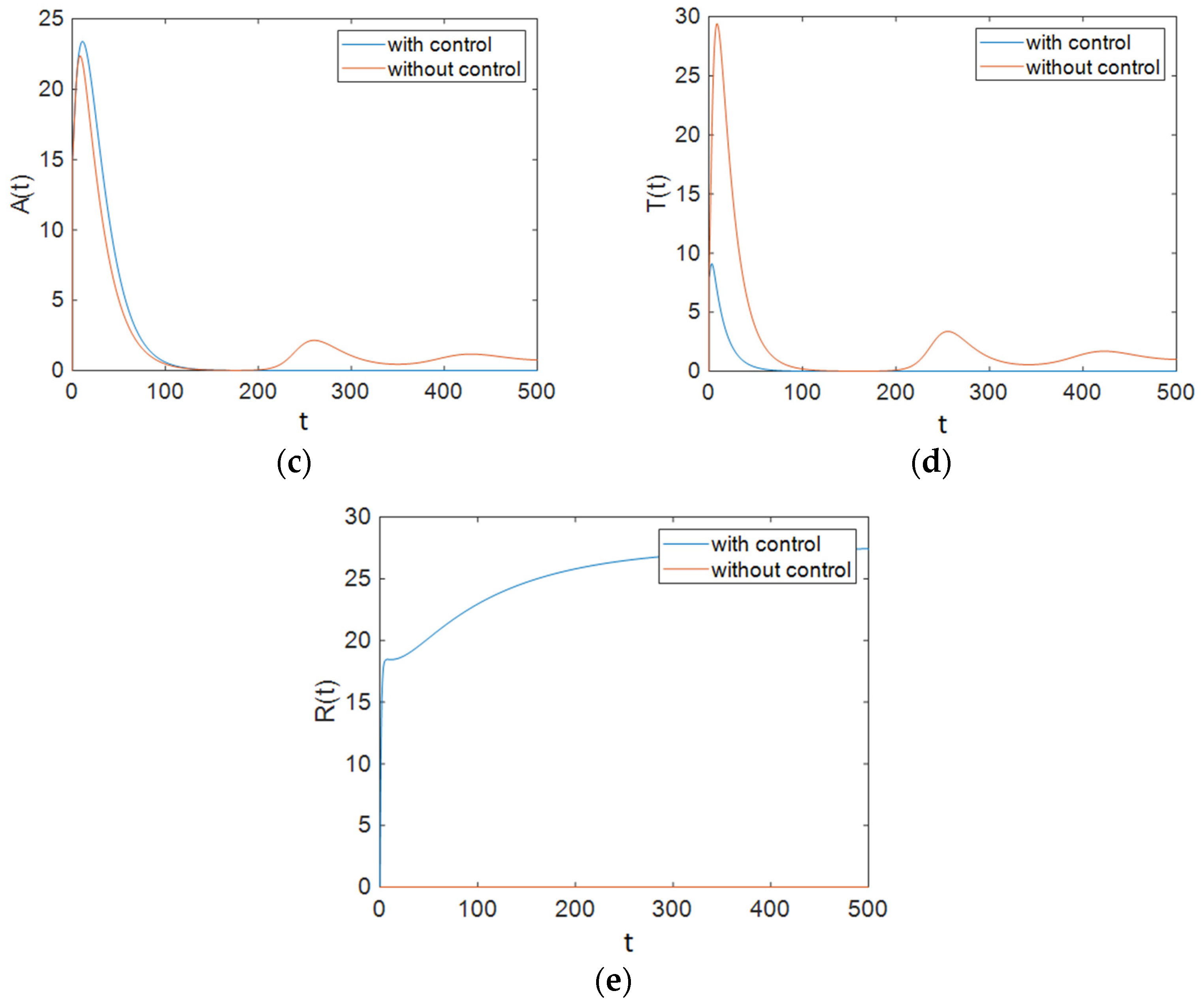
7.1. Strategy A: Control Using Treatment Alone

In this strategy, only the control u 2 was used to control the ART rate in the treated compartment per unit time. Figure 1 shows the results of the simulation of the case when only the control u 2 was applied to the system. It can be seen that for the aim of minimizing the population of the treated compartment, this control effort performed well, but it had detrimental effects on other states.
It can be seen in Figure 2 that control efforts were at 0 for approximately 100 days, and then they increased and reached 1; again, after a period of time, they returned to 0 linearly, and as is obvious, at the end of the simulation the control efforts u 1 had reached a zero value. It should be noted that for the simulations of the system without a controller, the values of control inputs were considered to be constant at u 1 = 1 ε 1 ,   u 2 = 0 ,   and   u 3 = 0 . Figure 3 depicts the time history of function L when Strategy A was applied to the system. Based on Figure 3, the optimal controller effectively reduced function L. As shown in Figure 1, this strategy (only the use of ART) could not improve the situation for all groups. Therefore, we need to apply prevention actions with ART, which are investigated in the next sections.

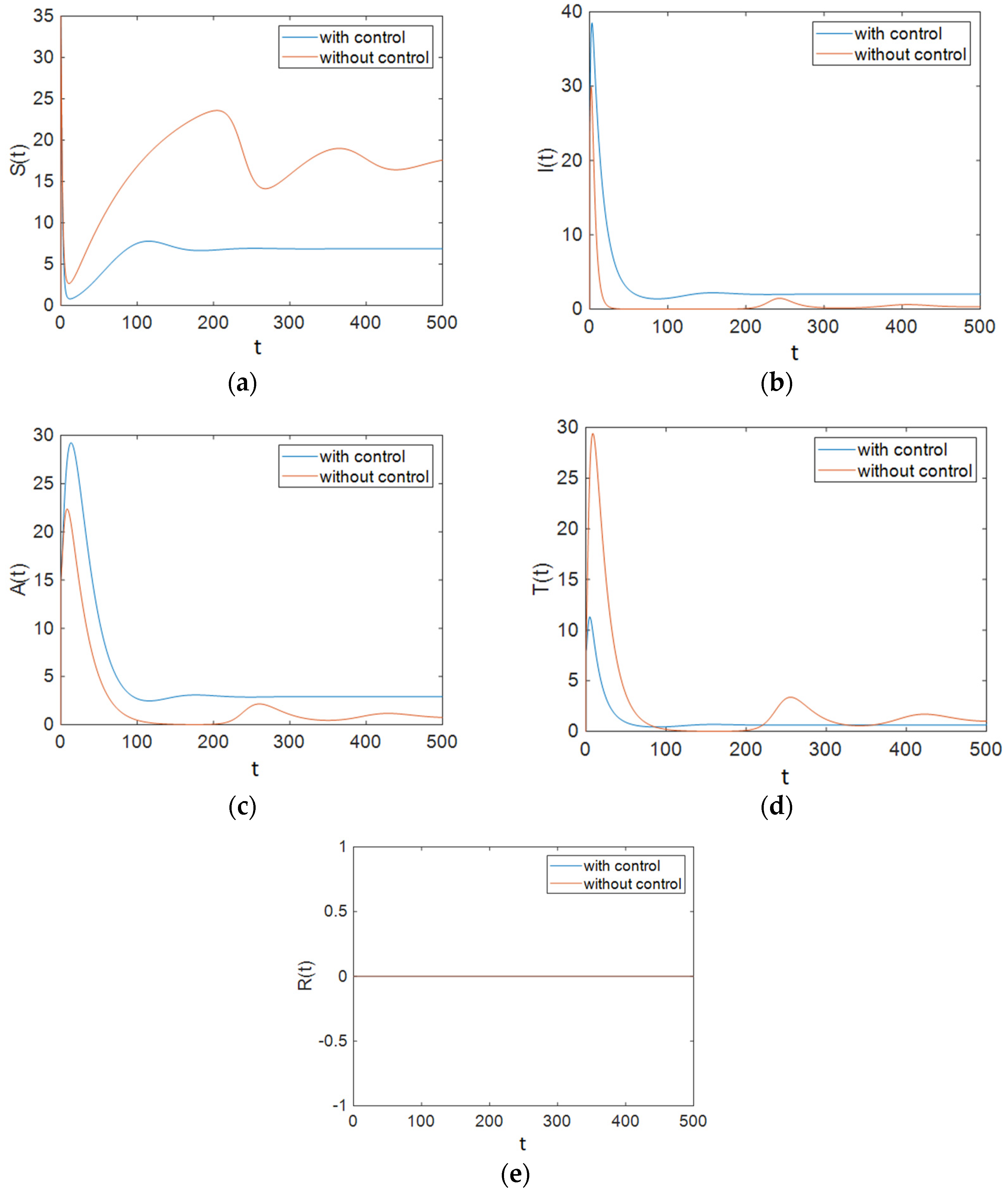
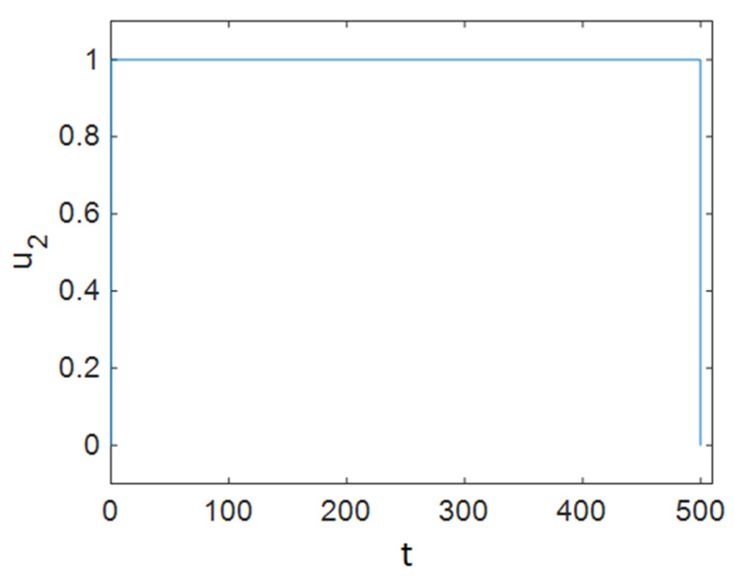
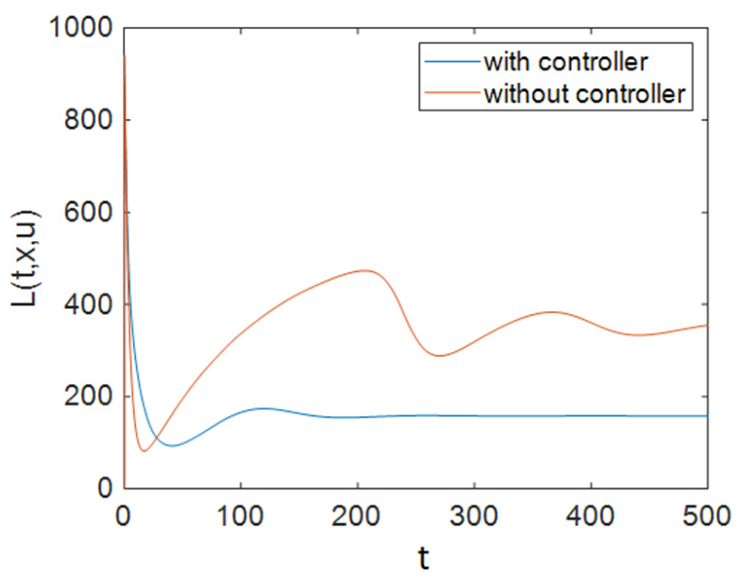
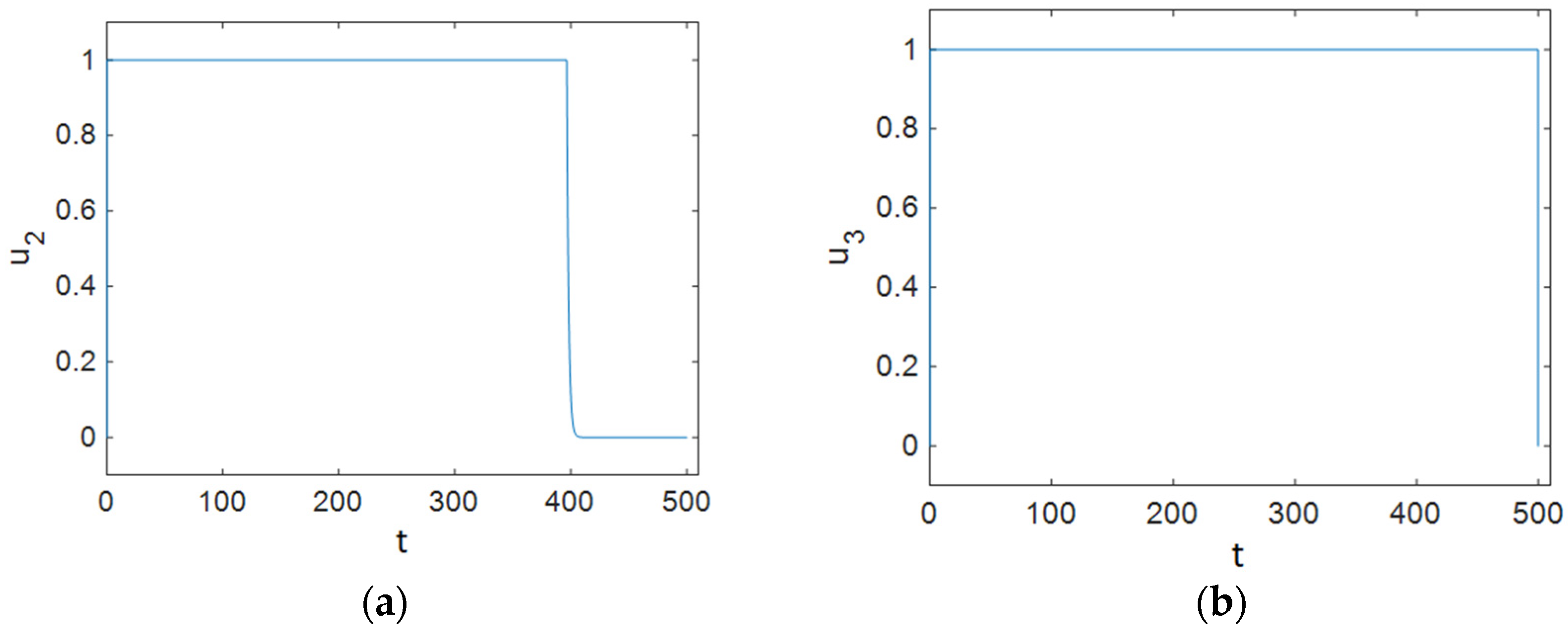
7.2. Strategy B: Control Using Treatment and Changes in People’s Sexual Habits

In this section, the behavior of the system was simulated for the case in which u 2 and u 3 are used to control the ART rate in the treated compartment per unit time and the proportion of susceptible people who have changed their sexual habits per unit time. The simulation results show the effectiveness of controlling the aforementioned parameters. Figure 4 shows that the population of susceptible people decreased significantly compared to the case with no control effort on the system, and it also shows that the number of people with full-blown AIDS did not change greatly from that in the case with no control effort. However, it can be observed that the population of the treated compartment reached zero over time. Furthermore, it can be seen that the number of people in the removed compartment increased remarkably.
As Figure 5 shows, ART was applied to individuals in the treated compartment at its maximum rate for half of the simulation time, and it dropped and reached zero after about 40 days; it can be concluded that people in the susceptible compartment must maintain changes in their sexual habits for most of the time, and it can be seen that the control efforts u3 decreased sharply at the end of the simulation and reached zero. Additionally, Figure 6 demonstrates that Strategy B effectively decreased the value of function L .

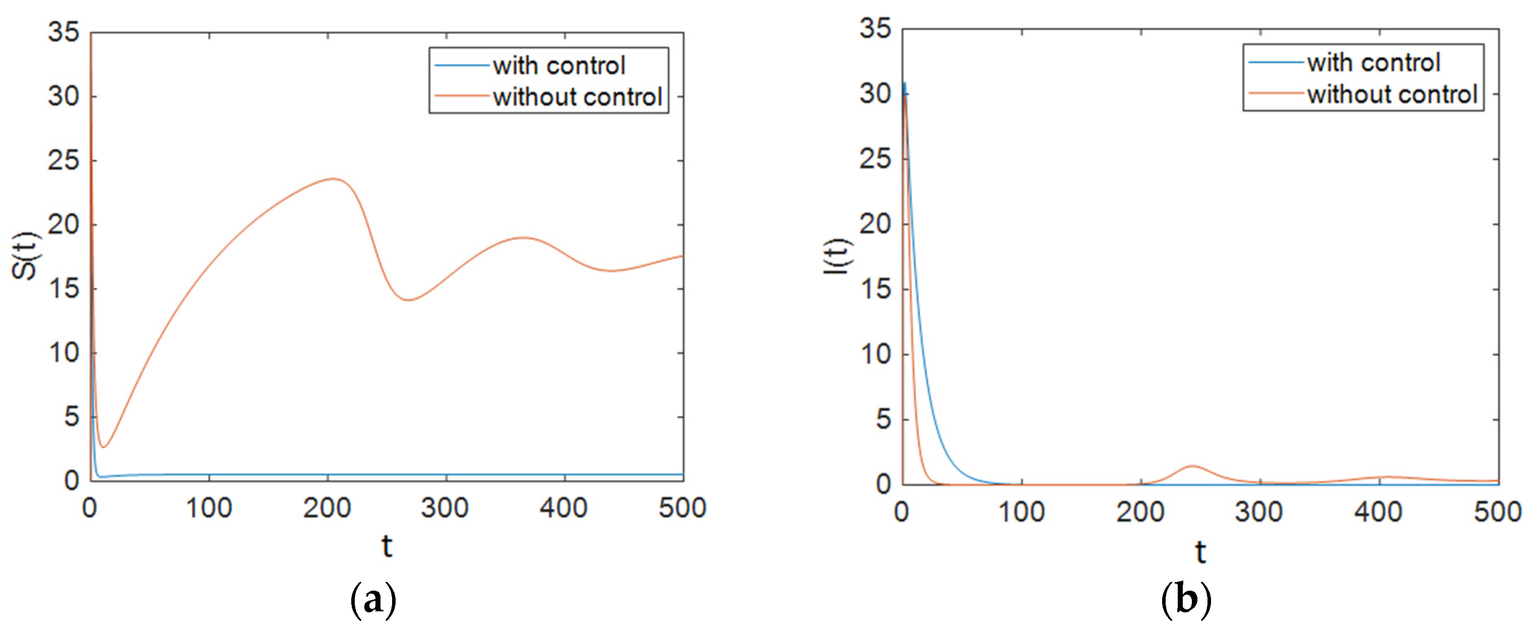
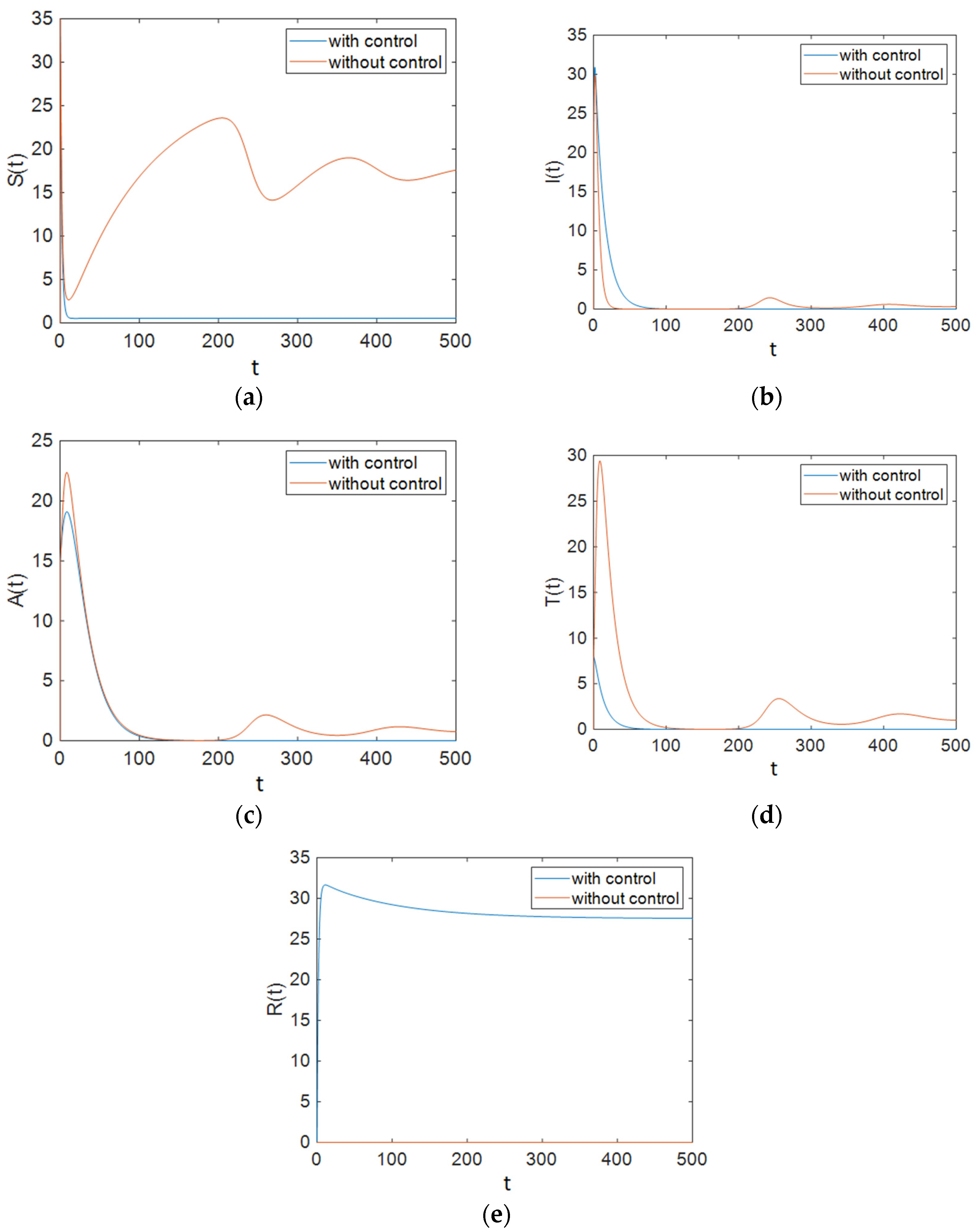
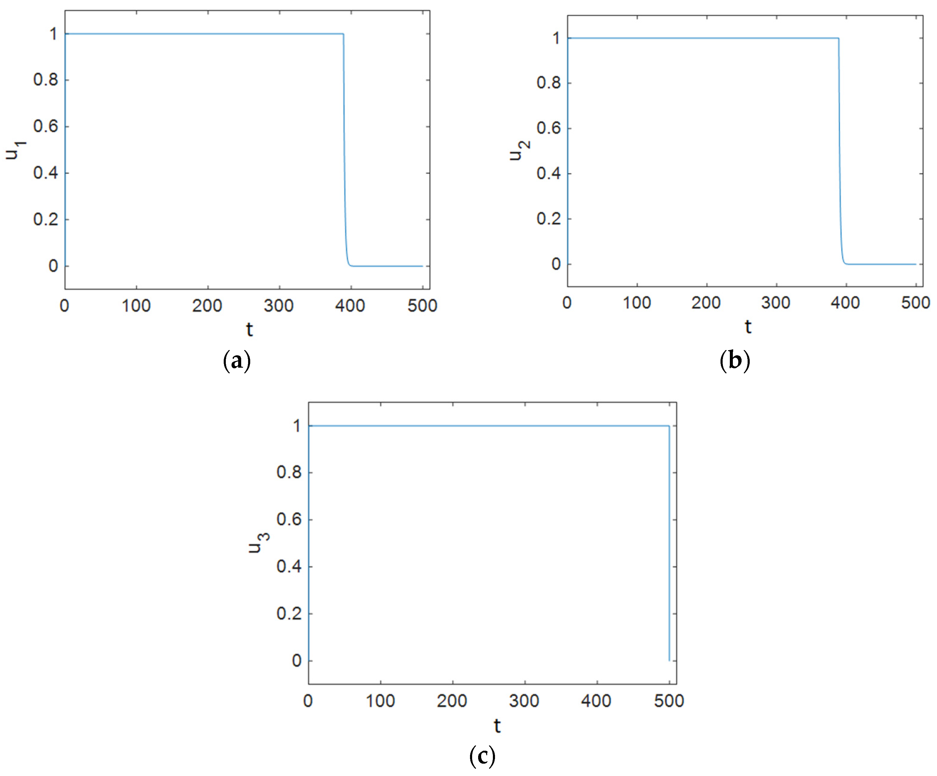
7.3. Strategy C: Control Using Prevention, Treatment, and Changes in Sexual Habits

In this case, all of the control efforts were applied to the system in order to minimize the predefined cost function, Equation (20). The results of the simulation show that the population of the susceptible compartment plunged; it remained at a low level and did not rise again. Besides this, the maximum number of infected people decreased compared to that in the case with no control effort, and the rate of decrease in the population of infectious individuals was faster. In addition, Figure 7 shows that the number of individuals with full-blown AIDS reached zero faster than it did in the case with no control effort. As can be observed in Figure 7, the maximum number of people in the treated compartment declined significantly, and the population decreased more sharply than it did in the case where no control effort was applied to the system. Figure 8 shows the time history of control efforts; it can be seen that control effort u 1 was at 1 for about 400 days, then it decreased delicately and reached 0, so it can be concluded that the contact rate of susceptible people and individuals in the infectious class must decrease by the use of condoms at a minimum rate. In addition, it is obvious that the rate of ART plunged after about 400 days and then reached zero slowly, so after about 400 days, there is no need for ART. Figure 8 shows that the individuals in the susceptible people compartment must maintain changes in their sexual habits until the end of the simulated time period. Figure 9 shows that the value of function L was reduced by Strategy C.

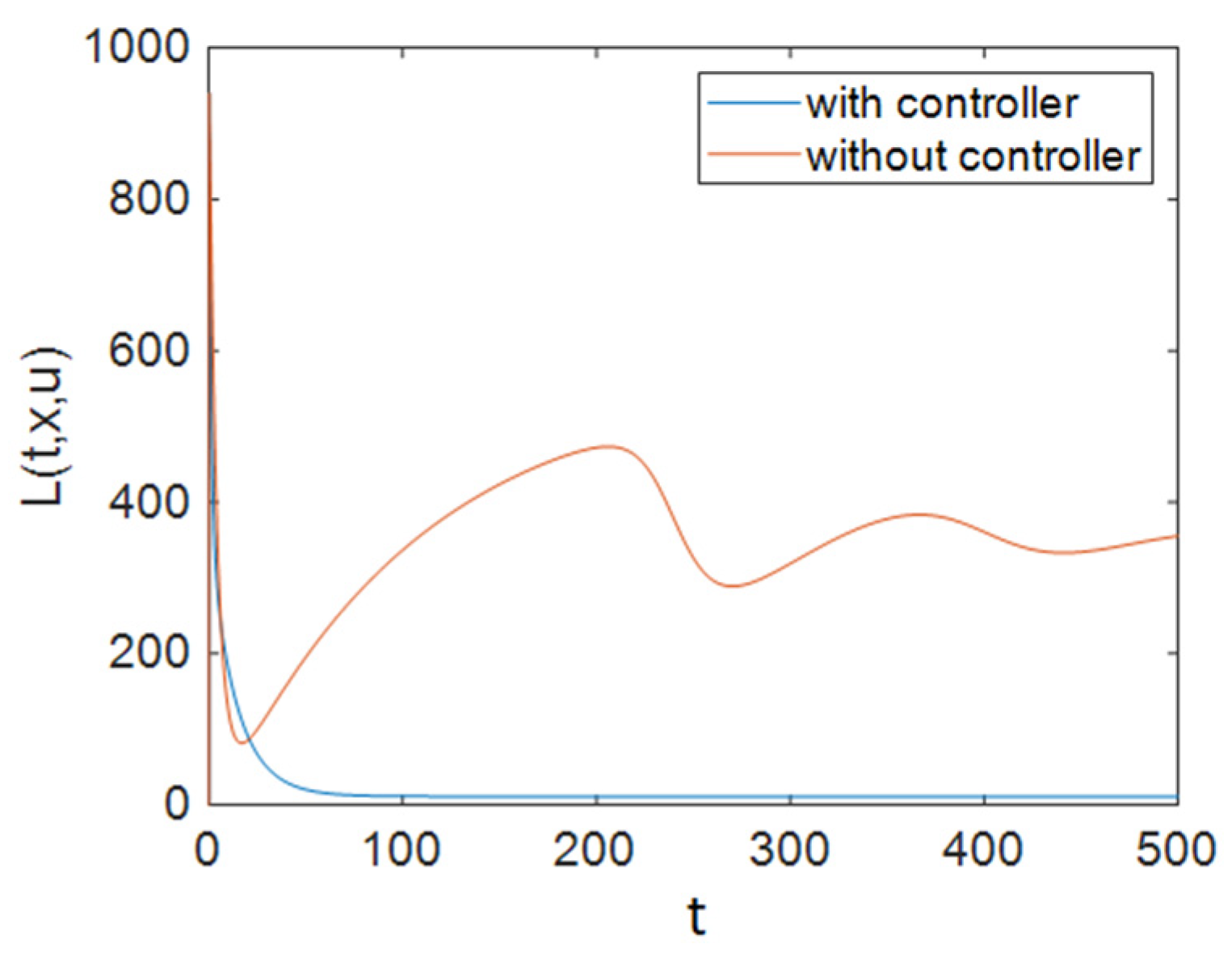
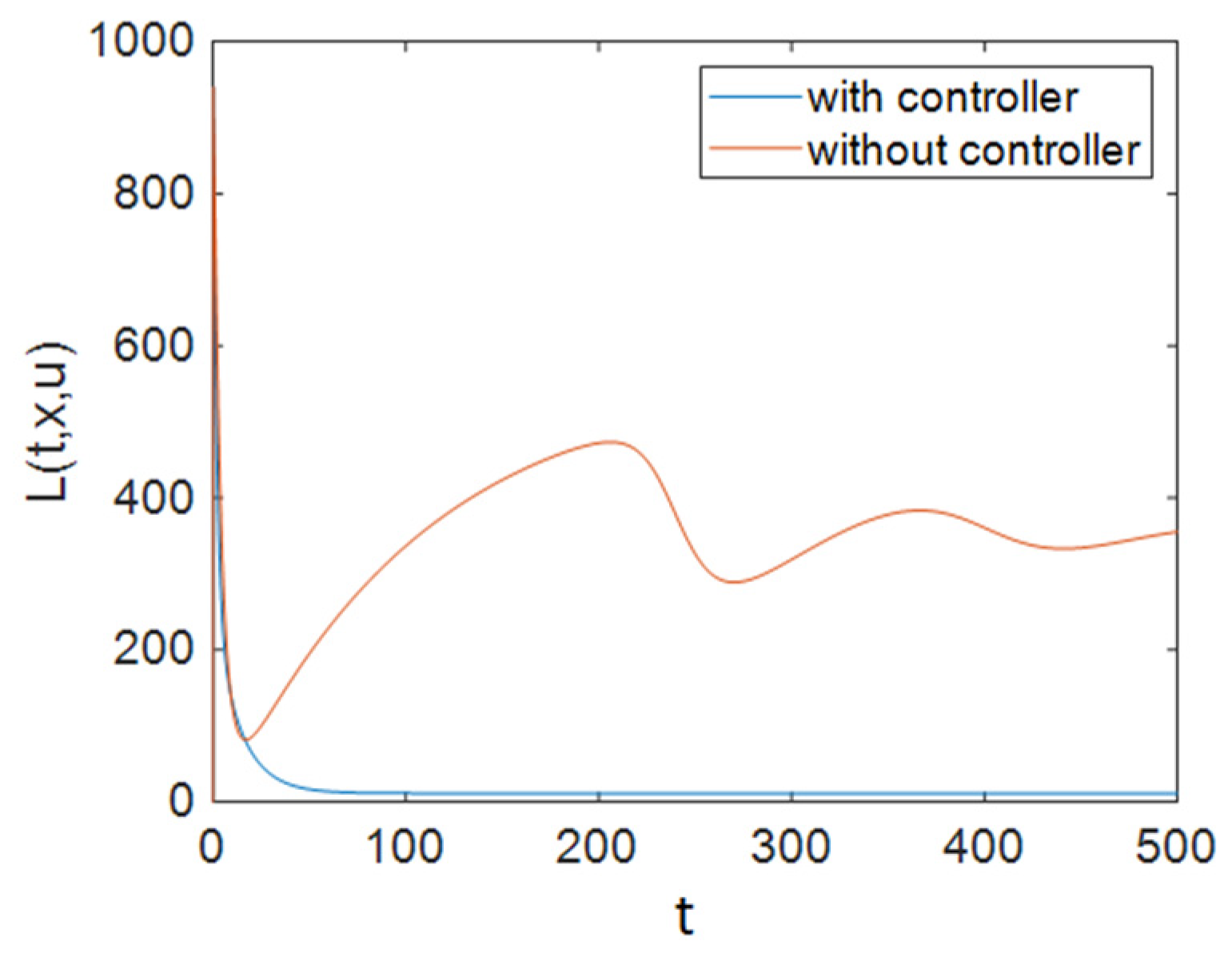
7.4. Comparing Different Strategies

As shown in Figure 1, Strategy A, which only applies ART, could not improve all groups’ situations. In Strategy B, the situation was better. As demonstrated in Figure 4, the population of susceptible people decreased significantly compared to that under Strategy A. In this strategy, the population of the treated compartment reached zero. Strategy C was the best one. In this strategy, the number of individuals with full-blown AIDS reached zero faster than it did in other strategies (especially compared with Strategy A). As shown in Figure 7, the maximum number of people in the treated compartment declined significantly, and the population of recovered people increased.
Also, to compare the results of all strategies easily, we can investigate the cost functions. As shown in Figure 3, Figure 6 and Figure 9, the value of the cost function in Strategy A was greater than those in Strategies B and C. Thus, it can be concluded that Strategy A is less effective than the other two investigated strategies.

8. Conclusions

In this paper, a CF fractional HIV/AIDS model was studied. In order to find control strategies to control disease, a sensitivity analysis was conducted. The results of the sensitivity analyses show that three parameters are more effective than others in controlling the disease. Using the results of these analyses, a modified model was proposed. The necessary conditions for the optimal control of the disease using control of the contact rate of susceptible and infectious people, control of the ART rate of the treated compartment population, and, finally, control of the rate of changes in the sexual habits of susceptible people were derived. Using a three-step fractional Adams–Bashforth scheme, simulations for four strategies were conducted, and the results of the simulations show that the best strategy is to use all of the control efforts simultaneously. Besides this, the results of the simulations show that the populations of the treated compartment and susceptible people class decreased at a higher rate under control strategies than when there was no controller. Furthermore, the population of the removed class increased notably. By considering the simulation results, it can be concluded that the proposed optimal controller is effective in controlling the disease. As a future suggestion, the advantages of the CF derivative can be used in the modeling of other biological systems. Furthermore, the optimal controller designed in the current paper is given as an open-loop controller. Hence, in a future study, by developing the proposed controller into a closed-loop one, its performance can be enhanced in dealing with modeling errors, uncertainties, and external disturbances.

Author Contributions

Conceptualization, H.W., H.J., M.-K.W., S.B., J.L., A.A.A.; Investigation, H.W., H.J., M.-K.W., S.B., J.L., A.A.A.; Methodology, H.W., H.J., M.-K.W., S.B., J.L., A.A.A.; Software, H.W., H.J., M.-K.W., S.B., J.L., A.A.A.; Supervision, H.W., H.J., M.-K.W., S.B., J.L., A.A.A.; Validation, H.W., H.J., M.-K.W., S.B., J.L., A.A.A.; Writing—original draft, H.W., H.J., M.-K.W., S.B., J.L., A.A.A.; Writing—review and editing, H.W., H.J., M.-K.W., S.B., J.L., A.A.A. All authors have read and agreed to the published version of the manuscript.

Funding

This research was supported by the Taif University Researchers Supporting Project number (TURSP-2020/77), Taif University, Taif, Saudi Arabia. Additionally, Jinping Liu was supported by the Research and development Program of key fields of Hunan Province under Grant No.2019SK2161.

Institutional Review Board Statement

Not applicable.

Informed Consent Statement

Not applicable.

Data Availability Statement

Not applicable.

Conflicts of Interest

The authors declare no conflict of interest.

References

  1. Elaiw, A.M.; Xia, X. HIV Dynamics: Analysis and Robust Multirate MPC-Based Treatment Schedules; Military Technical College: Cairo, Egypt, 2008; pp. 1–28. [Google Scholar]
  2. Egonmwan, A.O.; Okuonghae, D. Analysis of a mathematical model for tuberculosis with diagnosis. J. Appl. Math. Comput. 2019, 59, 129–162. [Google Scholar] [CrossRef]
  3. Pathak, S.; Maiti, A.; Samanta, G.P. Rich dynamics of an SIR epidemic model. Nonlinear Anal. Model. Control 2010, 15, 71–81. [Google Scholar] [CrossRef]
  4. Brauer, F. Some simple epidemic models. Math. Biosci. Eng. 2006, 3, 1. [Google Scholar] [CrossRef]
  5. Anderson, R.M.; Medley, G.F.; May, R.M.; Johnson, A.M. A preliminary study of the transmission dynamics of the human immunodeficiency virus (HIV), the causative agent of AIDS. Math. Med. Biol. J. IMA 1986, 3, 229–263. [Google Scholar] [CrossRef] [PubMed]
  6. Case, K.K.; Johnson, L.F.; Mahy, M.; Marsh, K.; Supervie, V.; Eaton, J.W. Summarizing the results and methods of the 2019 Joint United Nations Programme on HIV/AIDS HIV estimates. AIDS 2019, 33 (Suppl. 3), S197–S201. [Google Scholar] [CrossRef] [PubMed] [Green Version]
  7. Owolabi, K.M.; Atangana, A. Mathematical analysis and computational experiments for an epidemic system with nonlocal and nonsingular derivative. Chaos Solitons Fractals 2019, 126, 41–49. [Google Scholar] [CrossRef]
  8. Khajanchi, S.; Nieto, J.J. Mathematical modeling of tumor-immune competitive system, considering the role of time delay. Appl. Math. Comput. 2019, 340, 180–205. [Google Scholar] [CrossRef]
  9. Li, G.; Jin, Z. Global stability of a SEIR epidemic model with infectious force in latent, infected and immune period. Chaos Solitons Fractals 2005, 25, 1177–1184. [Google Scholar] [CrossRef]
  10. Tripathi, A.; Naresh, R.; Sharma, D. Modeling the effect of screening of unaware infectives on the spread of HIV infection. Appl. Math. Comput. 2007, 184, 1053–1068. [Google Scholar] [CrossRef]
  11. Jabbari, A.; Kheiri, H.; Jodayree Akbarfam, A.; Bekir, A. Dynamical analysis of the avian-human influenza epidemic model using multistage analytical method. Int. J. Biomath. 2016, 9, 1650090. [Google Scholar] [CrossRef]
  12. Bernoulli, D. Essai d’une nouvelle analyse de la mortalité causée par la petite vérole, et des avantages de l’inoculation pour la prévenir. Hist. Acad. R. Sci. Paris Mem. 1760, 811, 1–45. [Google Scholar]
  13. Ackermann, J.; Al-Bender, F.; Aliane, N.; Anderson, B.D.O.; Armstrong, B.S.R.; Astolfi, A.; Astrom, K.J.; Barhen, J.; Baumgartner, K.; Berenguel, M. 2008 Index IEEE Control Systems Magazine. IEEE Control Syst. Mag. 2008, 28, 148–156. [Google Scholar]
  14. Jahanshahi, H. Smooth control of HIV/AIDS infection using a robust adaptive scheme with decoupled sliding mode supervision. Eur. Phys. J. Spec. Top. 2018, 227, 707–718. [Google Scholar] [CrossRef]
  15. Bagley, R.L.; Calico, R.A. Fractional order state equations for the control of viscoelasticallydamped structures. J. Guid. Control Dyn. 1991, 14, 304–311. [Google Scholar] [CrossRef]
  16. Ahmed, E.; Hashish, A.; Rihan, F.A. On fractional order cancer model. J. Fract. Calc. Appl. Anal. 2012, 3, 1–6. [Google Scholar]
  17. Iyiola, O.S.; Zaman, F.D. A fractional diffusion equation model for cancer tumor. AIP Adv. 2014, 4, 107121. [Google Scholar] [CrossRef]
  18. Jahanshahi, H.; Yousefpour, A.; Munoz-Pacheco, J.M.; Moroz, I.; Wei, Z.; Castillo, O. A new multi-stable fractional-order four-dimensional system with self-excited and hidden chaotic attractors: Dynamic analysis and adaptive synchronization using a novel fuzzy adaptive sliding mode control method. Appl. Soft Comput. 2020, 87, 105943. [Google Scholar] [CrossRef]
  19. Wang, S.; He, S.; Yousefpour, A.; Jahanshahi, H.; Repnik, R.; Perc, M. Chaos and complexity in a fractional-order financial system with time delays. Chaos Solitons Fractals 2020, 131, 109521. [Google Scholar] [CrossRef]
  20. Soradi-Zeid, S.; Jahanshahi, H.; Yousefpour, A.; Bekiros, S. King algorithm: A novel optimization approach based on variable-order fractional calculus with application in chaotic financial systems. Chaos Solitons Fractals 2020, 132, 109569. [Google Scholar] [CrossRef]
  21. Wang, S.; Bekiros, S.; Yousefpour, A.; He, S.; Castillo, O.; Jahanshahi, H. Synchronization of fractional time-delayed financial system using a novel type-2 fuzzy active control method. Chaos Solitons Fractals 2020, 136, 109768. [Google Scholar] [CrossRef]
  22. Jahanshahi, H.; Yousefpour, A.; Munoz-Pacheco, J.M.; Kacar, S.; Pham, V.-T.; Alsaadi, F.E. A new fractional-order hyperchaotic memristor oscillator: Dynamic analysis, robust adaptive synchronization, and its application to voice encryption. Appl. Math. Comput. 2020, 383, 125310. [Google Scholar] [CrossRef]
  23. Chen, S.-B.; Jahanshahi, H.; Abba, O.A.; Solís-Pérez, J.E.; Bekiros, S.; Gómez-Aguilar, J.F.; Yousefpour, A.; Chu, Y.-M. The effect of market confidence on a financial system from the perspective of fractional calculus: Numerical investigation and circuit realization. Chaos Solitons Fractals 2020, 140, 110223. [Google Scholar] [CrossRef]
  24. Chen, S.-B.; Soradi-Zeid, S.; Jahanshahi, H.; Alcaraz, R.; Gómez-Aguilar, J.F.; Bekiros, S.; Chu, Y.-M. Optimal control of time-delay fractional equations via a joint application of radial basis functions and collocation method. Entropy 2020, 22, 1213. [Google Scholar] [CrossRef] [PubMed]
  25. Chen, S.-B.; Soradi-Zeid, S.; Alipour, M.; Chu, Y.-M.; Gomez-Aguilar, J.F.; Jahanshahi, H. Optimal control of nonlinear time-delay fractional differential equations with Dickson polynomials. Fractals 2020. [Google Scholar] [CrossRef]
  26. Jahanshahi, H.; Munoz-Pacheco, J.M.; Bekiros, S.; Alotaibi, N.D. A fractional-order SIRD model with time-dependent memory indexes for encompassing the multi-fractional characteristics of the COVID-19. Chaos Solitons Fractals 2021, 143, 110632. [Google Scholar] [CrossRef]
  27. Rajagopal, K.; Jahanshahi, H.; Jafari, S.; Weldegiorgis, R.; Karthikeyan, A.; Duraisamy, P. Coexisting attractors in a fractional order hydro turbine governing system and fuzzy PID based chaos control. Asian J. Control 2021, 23, 894–907. [Google Scholar] [CrossRef]
  28. Xiong, P.-Y.; Jahanshahi, H.; Alcaraz, R.; Chu, Y.-M.; Gómez-Aguilar, J.F.; Alsaadi, F.E. Spectral entropy analysis and synchronization of a multi-stable fractional-order chaotic system using a novel neural network-based chattering-free sliding mode technique. Chaos Solitons Fractals 2021, 144, 110576. [Google Scholar] [CrossRef]
  29. Jahanshahi, H.; Sajjadi, S.S.; Bekiros, S.; Aly, A.A. On the development of variable-order fractional hyperchaotic economic system with a nonlinear model predictive controller. Chaos Solitons Fractals 2021, 144, 110698. [Google Scholar] [CrossRef]
  30. Chu, Y.-M.; Bekiros, S.; Zambrano-Serrano, E.; Orozco-López, O.; Lahmiri, S.; Jahanshahi, H.; Aly, A.A. Artificial macro-economics: A chaotic discrete-time fractional-order laboratory model. Chaos Solitons Fractals 2021, 145, 110776. [Google Scholar] [CrossRef]
  31. Li, J.-F.; Jahanshahi, H.; Kacar, S.; Chu, Y.-M.; Gómez-Aguilar, J.F.; Alotaibi, N.D.; Alharbi, K.H. On the variable-order fractional memristor oscillator: Data security applications and synchronization using a type-2 fuzzy disturbance observer-based robust control. Chaos Solitons Fractals 2021, 145, 110681. [Google Scholar] [CrossRef]
  32. Wang, Y.-L.; Jahanshahi, H.; Bekiros, S.; Bezzina, F.; Chu, Y.-M.; Aly, A.A. Deep recurrent neural networks with finite-time terminal sliding mode control for a chaotic fractional-order financial system with market confidence. Chaos Solitons Fractals 2021, 146, 110881. [Google Scholar] [CrossRef]
  33. Ding, Y.; Ye, H. A fractional-order differential equation model of HIV infection of CD4+ T-cells. Math. Comput. Model. 2009, 50, 386–392. [Google Scholar] [CrossRef]
  34. Rihan, F.A. Numerical modeling of fractional-order biological systems. Hindawi Abstr. Appl. Anal. 2013, 2013. [Google Scholar] [CrossRef] [Green Version]
  35. Pinto, C.M.A.; Carvalho, A.R.M. New findings on the dynamics of HIV and TB coinfection models. Appl. Math. Comput. 2014, 242, 36–46. [Google Scholar] [CrossRef] [Green Version]
  36. Dutta, A.; Adak, A.; Gupta, P.K. Analysis of fractional-order deterministic HIV/AIDS model during drug therapy treatment. In Soft Computing for Problem Solving; Springer: Cham, Switzerland, 2020; pp. 1–8. [Google Scholar]
  37. Losada, J.; Nieto, J.J. Properties of a new fractional derivative without singular kernel. Prog. Fract. Differ. Appl. 2015, 1, 87–92. [Google Scholar]
  38. Caputo, M.; Fabrizio, M. A new definition of fractional derivative without singular kernel. Prog. Fract. Differ. Appl. 2015, 1, 1–13. [Google Scholar]
  39. Alsaedi, A.; Nieto, J.J.; Venktesh, V. Fractional electrical circuits. Adv. Mech. Eng. 2015, 7. [Google Scholar] [CrossRef]
  40. Singh, J.; Kumar, D.; Baleanu, D. New aspects of fractional Biswas–Milovic model with Mittag-Leffler law. Math. Model. Nat. Phenom. 2019, 14, 303. [Google Scholar] [CrossRef] [Green Version]
  41. Kumar, D.; Tchier, F.; Singh, J.; Baleanu, D. An efficient computational technique for fractal vehicular traffic flow. Entropy 2018, 20, 259. [Google Scholar] [CrossRef] [Green Version]
  42. Owolabi, K.M.; Atangana, A. Analysis and application of new fractional Adams–Bashforth scheme with Caputo–Fabrizio derivative. Chaos Solitons Fractals 2017, 105, 111–119. [Google Scholar] [CrossRef]
  43. Kumar, D.; Singh, J.; Al Qurashi, M.; Baleanu, D. Analysis of logistic equation pertaining to a new fractional derivative with non-singular kernel. Adv. Mech. Eng. 2017, 9. [Google Scholar] [CrossRef]
  44. Tateishi, A.A.; Ribeiro, H.V.; Lenzi, E.K. The role of fractional time-derivative operators on anomalous diffusion. Front. Phys. 2017, 5, 52. [Google Scholar] [CrossRef] [Green Version]
  45. Atangana, A.; Alkahtani, B. Analysis of the Keller–Segel model with a fractional derivative without singular kernel. Entropy 2015, 17, 4439–4453. [Google Scholar] [CrossRef]
  46. Diethelm, K. The Analysis of Fractional Differential Equations: An Application-Oriented Exposition Using Differential Operators of Caputo Type; Springer Science & Business Media: Berlin, Germany, 2010. [Google Scholar]
  47. Atangana, A.; Gómez-Aguilar, J.F. Decolonisation of fractional calculus rules: Breaking commutativity and associativity to capture more natural phenomena. Eur. Phys. J. Plus 2018, 133, 166. [Google Scholar] [CrossRef]
  48. Atangana, A. Blind in a commutative world: Simple illustrations with functions and chaotic attractors. Chaos Solitons Fractals 2018, 114, 347–363. [Google Scholar] [CrossRef]
  49. Moore, E.J.; Sirisubtawee, S.; Koonprasert, S. A Caputo–Fabrizio fractional differential equation model for HIV/AIDS with treatment compartment. Adv. Differ. Equ. 2019, 2019, 200. [Google Scholar] [CrossRef] [Green Version]
  50. Liu, J.; Zhao, S.; Xie, Y.; Gui, W.; Tang, Z.; Ma, T.; Niyoyita, J.P. Learning local Gabor pattern-based discriminative dictionary of froth images for flotation process working condition monitoring. IEEE Trans. Ind. Inform. 2020, 17, 4437–4448. [Google Scholar] [CrossRef]
  51. Liu, J.; He, J.; Xie, Y.; Gui, W.; Tang, Z.; Ma, T.; He, J.; Niyoyita, J.P. Illumination-Invariant flotation froth color measuring via Wasserstein distance-based CycleGAN with structure-preserving constraint. IEEE Trans. Cybern. 2020, 51, 839–852. [Google Scholar] [CrossRef]
  52. Kosari, A.; Jahanshahi, H.; Razavi, S.A. Optimal FPID control approach for a docking maneuver of two spacecraft: Translational motion. J. Aerosp. Eng. 2017, 30, 04017011. [Google Scholar] [CrossRef]
  53. Kosari, A.; Jahanshahi, H.; Razavi, S.A. An optimal fuzzy PID control approach for docking maneuver of two spacecraft: Orientational motion. Eng. Sci. Technol. Int. J. 2017, 20, 293–309. [Google Scholar] [CrossRef] [Green Version]
  54. Jahanshahi, H.; Chen, D.; Chu, Y.-M.; Gómez-Aguilar, J.F.; Aly, A.A. Enhancement of the performance of nonlinear vibration energy harvesters by exploiting secondary resonances in multi-frequency excitations. Eur. Phys. J. Plus 2021, 136, 1–22. [Google Scholar] [CrossRef]
  55. Bekiros, S.; Jahanshahi, H.; Bezzina, F.; Aly, A.A. A novel fuzzy mixed H2/H∞ optimal controller for hyperchaotic financial systems. Chaos Solitons Fractals 2021, 146, 110878. [Google Scholar] [CrossRef]
  56. Jahanshahi, H.; Yousefpour, A.; Wei, Z.; Alcaraz, R.; Bekiros, S. A financial hyperchaotic system with coexisting attractors: Dynamic investigation, entropy analysis, control and synchronization. Chaos Solitons Fractals 2019, 126, 66–77. [Google Scholar] [CrossRef]
  57. Jahanshahi, H.; Shahriari-Kahkeshi, M.; Alcaraz, R.; Wang, X.; Singh, V.P.; Pham, V.-T. Entropy analysis and neural network-based adaptive control of a non-equilibrium four-dimensional chaotic system with hidden attractors. Entropy 2019, 21, 156. [Google Scholar] [CrossRef] [Green Version]
  58. Jahanshahi, H.; Rajagopal, K.; Akgul, A.; Sari, N.N.; Namazi, H.; Jafari, S. Complete analysis and engineering applications of a megastable nonlinear oscillator. Int. J. NonLinear Mech. 2018, 107, 126–136. [Google Scholar] [CrossRef]
  59. Ying, H.; Lin, F.; MacArthur, R.D.; Cohn, J.A.; Barth-Jones, D.C.; Ye, H.; Crane, L.R. A self-learning fuzzy discrete event system for HIV/AIDS treatment regimen selection. IEEE Trans. Syst. Man Cybern. Part B Cybern. 2007, 37, 966–979. [Google Scholar] [CrossRef]
  60. Ying, H.; Lin, F.; MacArthur, R.D.; Cohn, J.A.; Barth-Jones, D.C.; Ye, H.; Crane, L.R. A fuzzy discrete event system approach to determining optimal HIV/AIDS treatment regimens. IEEE Trans. Inf. Technol. Biomed. 2006, 10, 663–676. [Google Scholar] [CrossRef]
  61. Brandt, M.E.; Chen, G. Feedback control of a biodynamical model of HIV-1. IEEE Trans. Biomed. Eng. 2001, 48, 754–759. [Google Scholar] [CrossRef]
  62. Jeffrey, A.M.; Xia, X.; Craig, I.K. When to initiate HIV therapy: A control theoretic approach. IEEE Trans. Biomed. Eng. 2003, 50, 1213–1220. [Google Scholar] [CrossRef]
  63. Kwon, H.-D. Optimal treatment strategies derived from a HIV model with drug-resistant mutants. Appl. Math. Comput. 2007, 188, 1193–1204. [Google Scholar] [CrossRef]
  64. Kirschner, D.; Lenhart, S.; Serbin, S. Optimal control of the chemotherapy of HIV. J. Math. Biol. 1997, 35, 775–792. [Google Scholar] [CrossRef] [PubMed] [Green Version]
  65. Barão, M.; Lemos, J.M. Nonlinear control of HIV-1 infection with a singular perturbation model. Biomed. Signal Process. Control 2007, 2, 248–257. [Google Scholar] [CrossRef] [Green Version]
  66. Ge, S.S.; Tian, Z.; Lee, T.H. Nonlinear control of a dynamic model of HIV-1. IEEE Trans. Biomed. Eng. 2005, 52, 353–361. [Google Scholar] [CrossRef]
  67. Ko, J.H.; Kim, W.H.; Chung, C.C. Optimized structured treatment interruption for HIV therapy and its performance analysis on controllability. IEEE Trans. Biomed. Eng. 2006, 53, 380–386. [Google Scholar] [CrossRef]
  68. Singh, J.; Kumar, D.; Hammouch, Z.; Atangana, A. A fractional epidemiological model for computer viruses pertaining to a new fractional derivative. Appl. Math. Comput. 2018, 316, 504–515. [Google Scholar] [CrossRef]
  69. Bani-Yaghoub, M.; Gautam, R.; Shuai, Z.; Van Den Driessche, P.; Ivanek, R. Reproduction numbers for infections with free-living pathogens growing in the environment. J. Biol. Dyn. 2012, 6, 923–940. [Google Scholar] [CrossRef]
  70. Van den Driessche, P.; Watmough, J. Reproduction numbers and sub-threshold endemic equilibria for compartmental models of disease transmission. Math. Biosci. 2002, 180, 29–48. [Google Scholar] [CrossRef]
  71. Zhang, J.; Ma, X.; Li, L. Optimality conditions for fractional variational problems with Caputo-Fabrizio fractional derivatives. Adv. Differ. Equ. 2017, 2017, 357. [Google Scholar] [CrossRef] [Green Version]
  72. Kheiri, B.; Abdalla, A.; Osman, M.; Ahmed, S.; Hassan, M.; Bachuwa, G. Vitamin D deficiency and risk of cardiovascular diseases: A narrative review. Clin. Hypertens. 2018, 24, 9. [Google Scholar] [CrossRef]
Figure 1. The number of individuals under Strategy A, which includes the use of ART: (a) Susceptible patients; (b) People who are infectious; (c) Individuals for whom the treatment is not effective; (d) Individuals being treated with ART and for whom the treatment is effective; (e) Individuals who have changed their sexual habits sufficiently.
Entropy 23 00610 g001
Figure 2. Time history of the optimal control effort u 2 (ART treatment).
Entropy 23 00610 g002
Figure 3. The time history of function L when applying Strategy A.
Entropy 23 00610 g003
Figure 4. The number of individuals under Strategy B, which includes ART treatment and changes in the sexual habits of susceptible patients: (a) Susceptible patients; (b) People who are infectious; (c) Individuals for whom the treatment is not effective; (d) Individuals being treated with ART for whom the treatment is effective; (e) Individuals who have changed their sexual habits sufficiently.
Entropy 23 00610 g004aEntropy 23 00610 g004b
Figure 5. Time history of the optimal control efforts: (a) u 2   ( ART   treatment ) ; (b) u 3   ( changes   in   the   sexual   habits   of   susceptible   patients ) .
Entropy 23 00610 g005
Figure 6. The time history of function L when applying Strategy B.
Entropy 23 00610 g006
Figure 7. The number of individuals under Strategy C, which includes condom use, ART treatment, and changes   in   the   sexual   habits   of   susceptible   patients : (a) Susceptible patients; (b) People who are infectious; (c) Individuals for whom the treatment is not effective; (d) Individuals being treated with ART for whom the treatment is effective; (e) Individuals who have changed their sexual habits sufficiently.
Entropy 23 00610 g007
Figure 8. Time history of the optimal control efforts: (a) u 1   ( condom   use ) ; (b) u 2   ( ART   treatment ) ; (c) u 3   ( changes   in   the   sexual   habits   of   susceptible   patients ) .
Entropy 23 00610 g008
Figure 9. The time history of function L when applying Strategy C.
Entropy 23 00610 g009
Table 1. The system parameters [49].
ParameterDescriptionValue
Λ The recruitment of susceptible people into the population0.55
β The contact rate between susceptible and infectious people0.03
d The natural death rate0.0196
k 1 The rate at which leave the infectious class and become individuals with full-blown AIDS0.15
k 2 The rate at which people with HIV receive treatment0.35
α 1 The rate at which treated individuals leave this compartment and return to the infectious compartment0.08
α 2 The rate at which individuals in the treated compartment leave this class and enter the AIDS compartment0.03
δ 1 The disease-induced death rate for individuals of the AIDS compartment0.0909
δ 2 The disease-induced death rate for individuals of the treated compartment0.0667
μ 1 The rate at which susceptible people change their sexual habits0.03
Table 2. Sensitivity indices of to the parameters of the model.
ParameterDescriptionSensitivity Index
Λ The recruitment of susceptible individuals into the population1
β The contact rate between susceptible and infectious individuals1
α 1 The rate at which treated individuals leave this compartment and return to the infectious compartment−0.7231
α 2 The rate at which individuals in the treated compartment leave this class and enter the AIDS compartment0.1865
δ 1 The disease-induced death rate for individuals of the AIDS compartment0.0
δ 2 The disease-induced death rate for individuals of the treated compartment0.4147
μ 1 The rate at which susceptible people change their sexual habits0.1333
Table 3. The sensitivity indices of the state variables at the endemic equilibrium point.
Parameter S * I * T *
Λ 0.00000.12370.1237
β −1.0000−0.8762−0.8762
α 1 0.7231−0.0894−0.4970
α 2 −0.18650.0230−0.1297
δ 1 0.00000.00000.0000
δ 2 −0.41470.0513−0.2885
μ 1 −0.73820.62130.6213
Publisher’s Note: MDPI stays neutral with regard to jurisdictional claims in published maps and institutional affiliations.

