
Generalized Structure Functions and Multifractal Detrended Fluctuation Analysis Applied to Vegetation Index Time Series: An Arid Rangeland Study

 ,
,  ,
,  ,
,  , ,
, , 
Abstract
1. Introduction
2. Area of Study, Data Collection and Methods
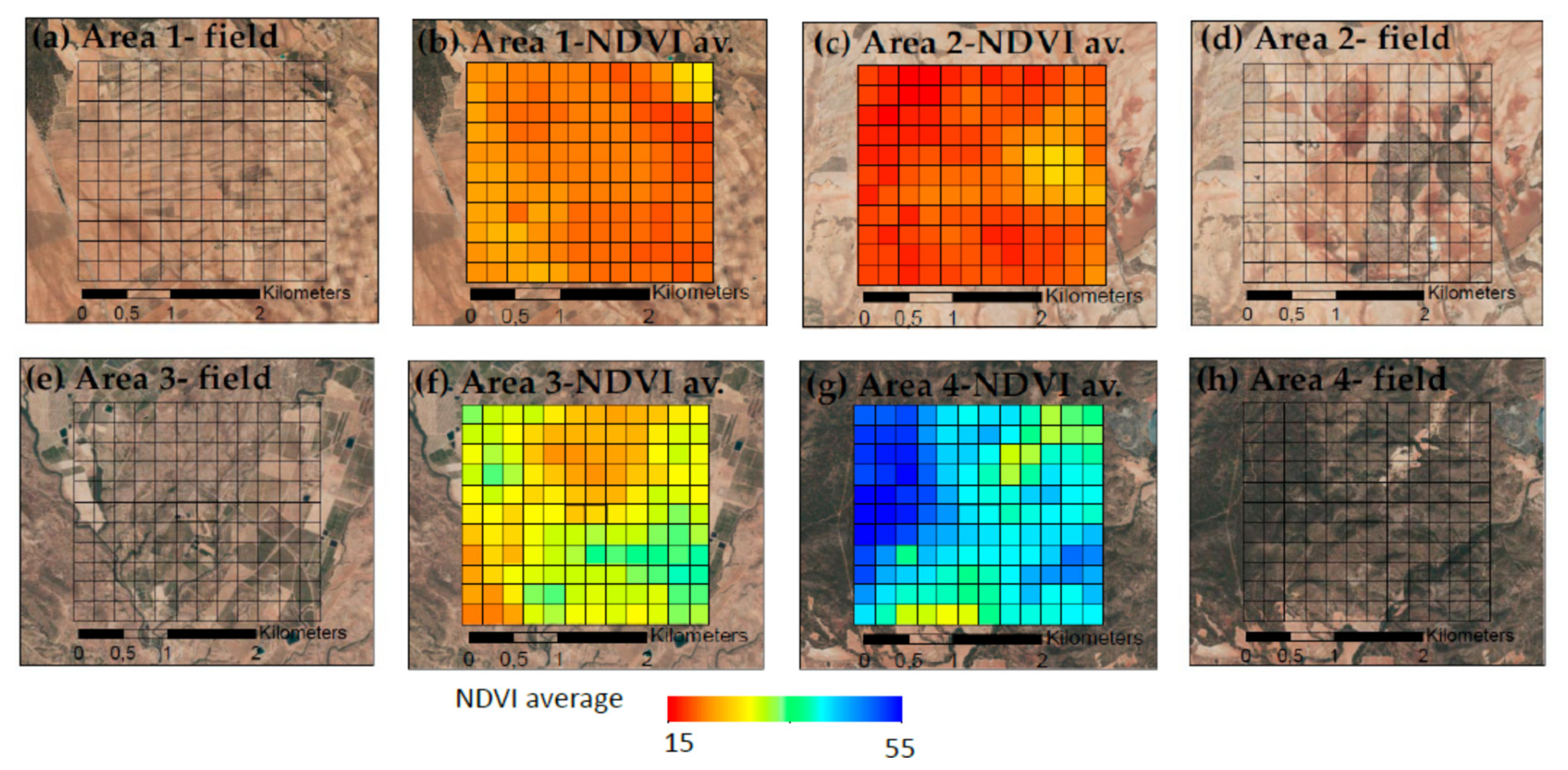
2.1. Area of Study
2.2. NDVI Data Collection
2.3. Methods
2.3.1. Temporal Trend Analysis
2.3.2. Hurst Index
2.3.3. Generalized Structure Function
2.3.4. Multifractal Detrended Fluctuation Analysis
3. Results
3.1. Temporal Trend Analysis
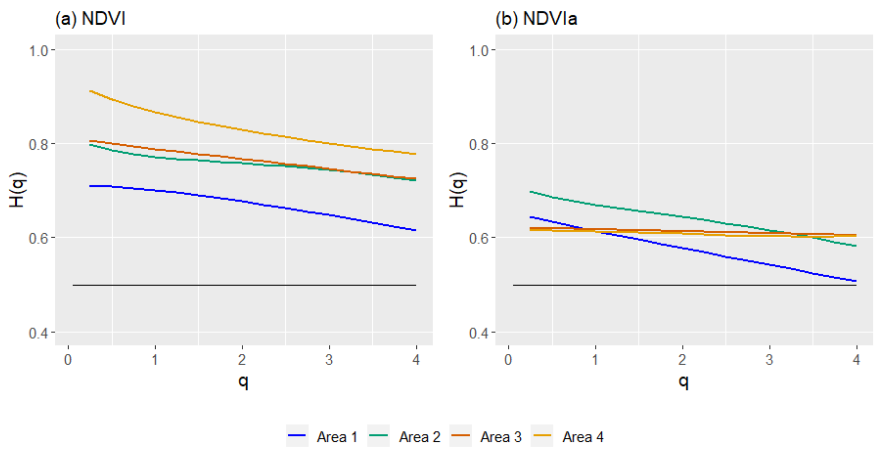
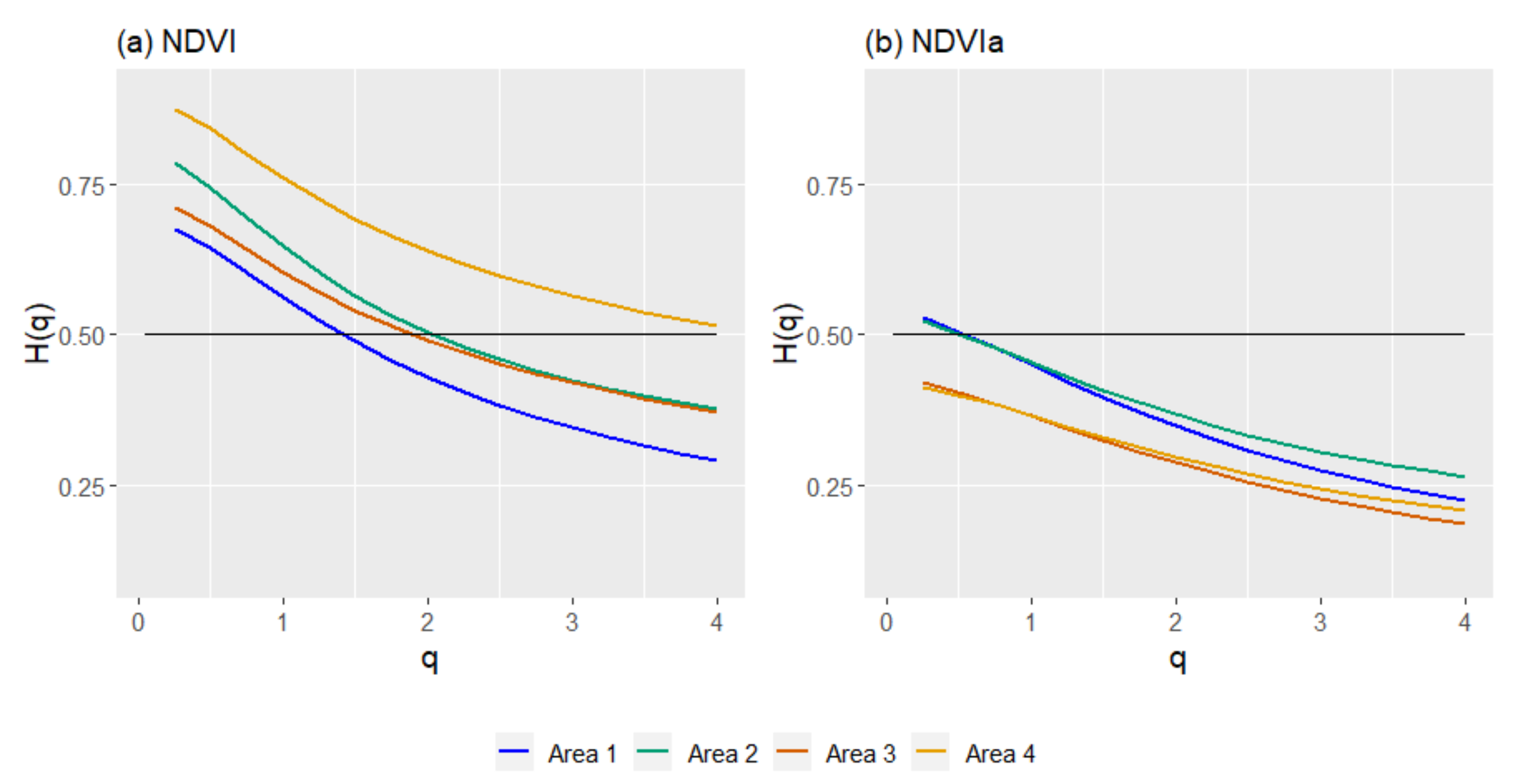
3.2. Hurst Index
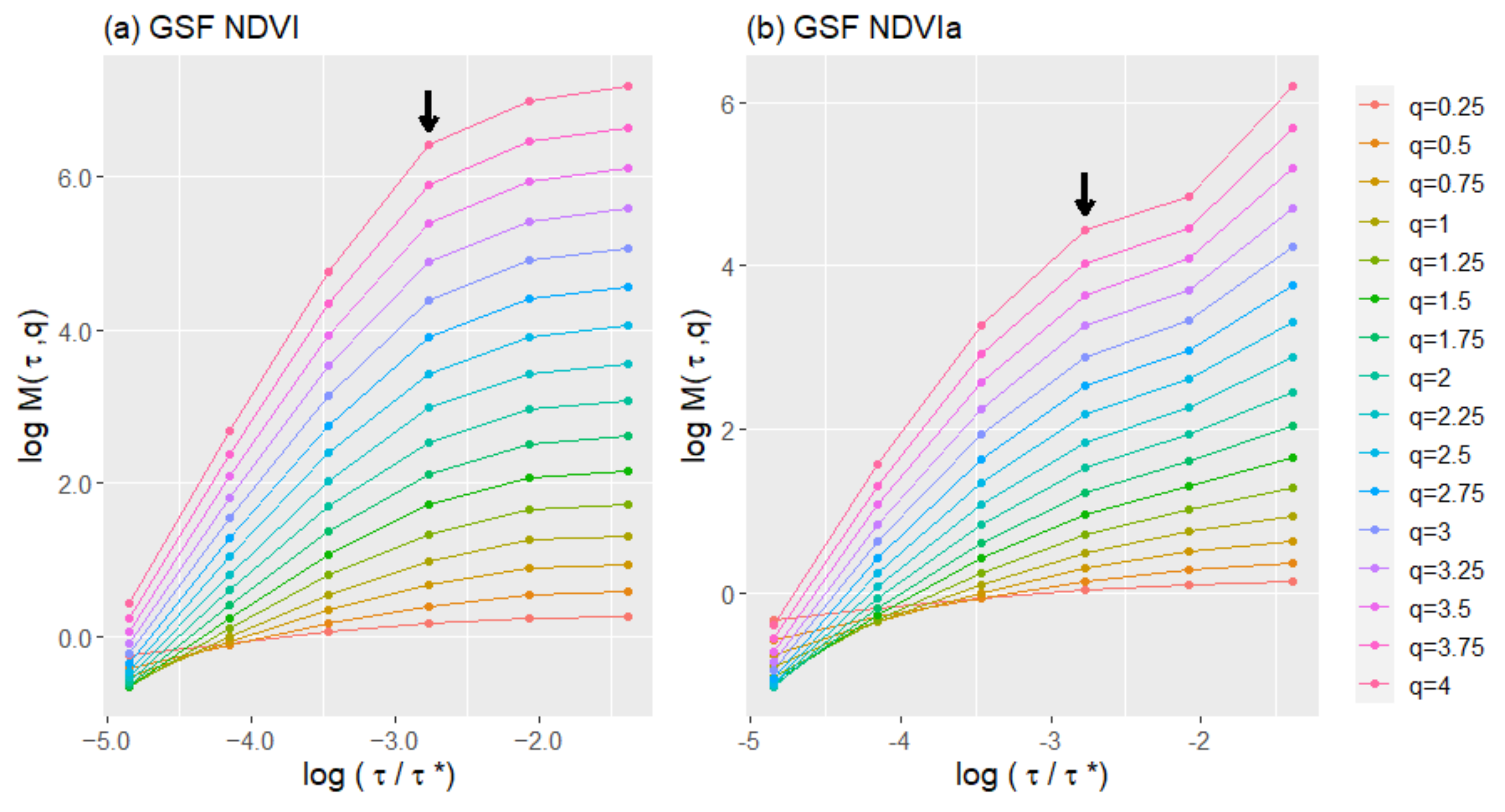
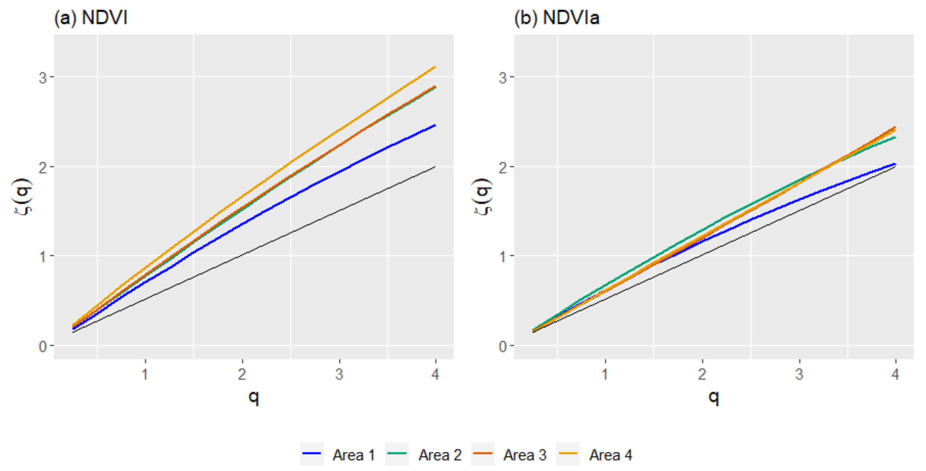
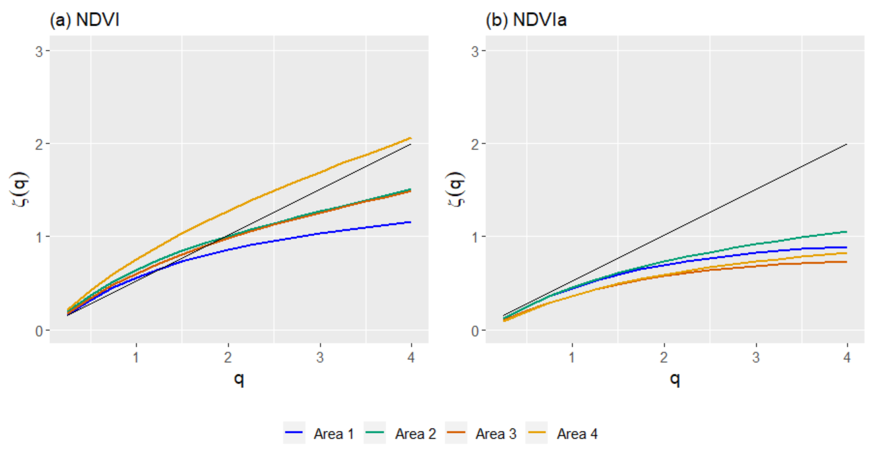
3.3. Generalized Structure Function
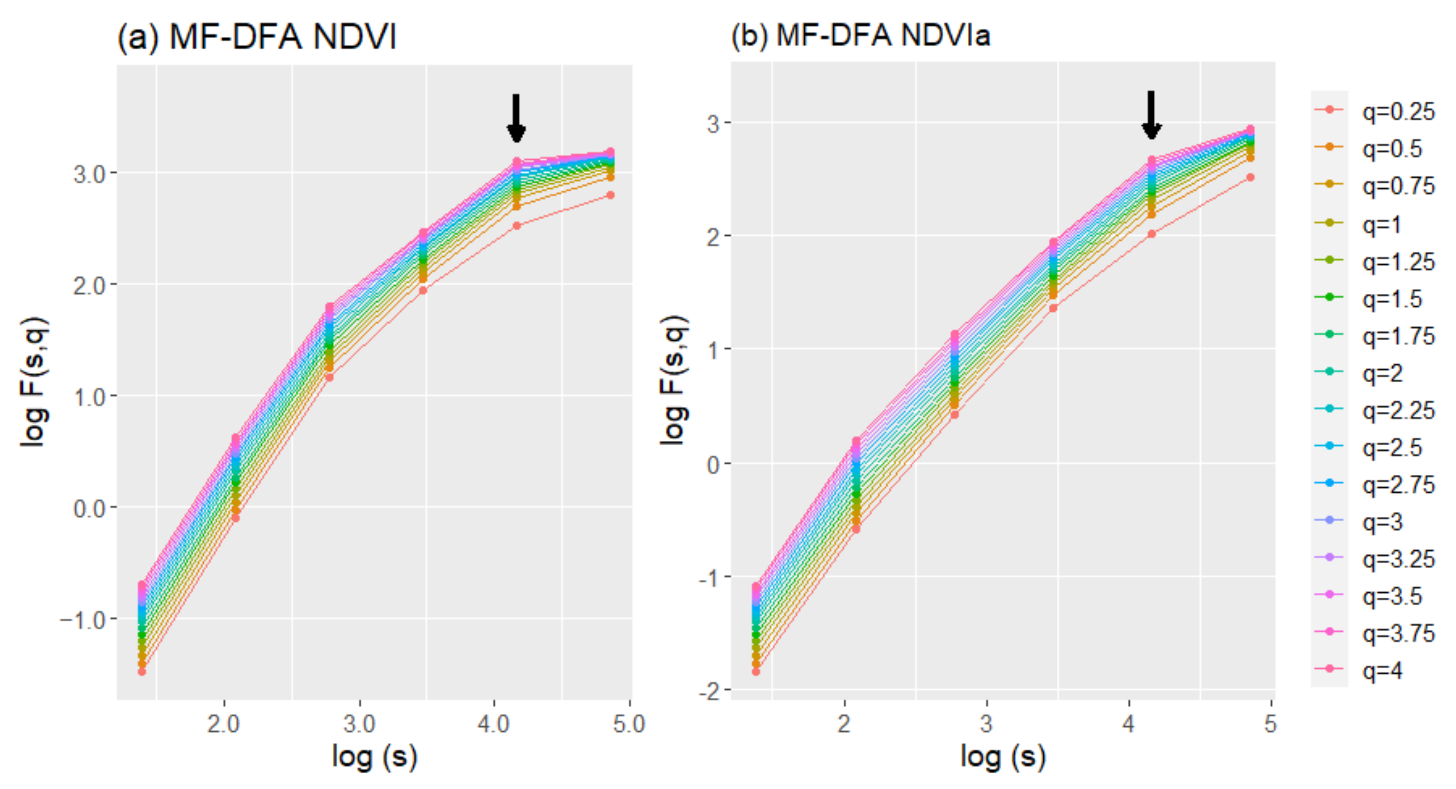
3.4. Multifractal Detrended Fluctuation Analysis
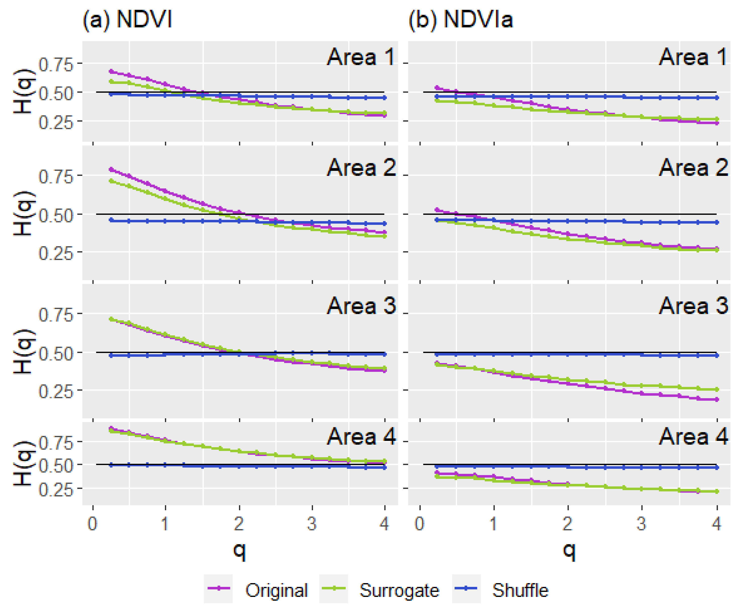
3.5. Sources of Multifractality
4. Discussion
5. Conclusions
Author Contributions
Funding
Institutional Review Board Statement
Informed Consent Statement
Data Availability Statement
Acknowledgments
Conflicts of Interest
References
- Ellis, E.C.; Ramankutty, N. Putting people in the map: Anthropogenic biomes of the world. Front. Ecol. Environ. 2008, 6, 439–447. [Google Scholar] [CrossRef]
- Zerga, B. Degradation of Rangelands and Rehabilitation efforts in Ethiopia: The case of Afar rangelands. J. Mech. Ind. Eng. Res. 2015, 4, 45. [Google Scholar]
- Pickup, G.; Bastin, G.N.; Chewings, V.H. Identifying trends in land degradation in non-equilibrium rangelands. J. Appl. Ecol. 1998, 35, 365–377. [Google Scholar] [CrossRef]
- Guichard, F.; Gouhier, T.C. Non-equilibrium spatial dynamics of ecosystems. Math. Biosci. 2014, 255, 1–10. [Google Scholar] [CrossRef] [PubMed]
- Curran, P.J.; Dungan, J.L.; Gholz, H.L. Seasonal LAI in slash pine estimated with Landsat TM. Remote Sens. Environ. 1992, 39, 3–13. [Google Scholar] [CrossRef]
- Henebry, G.M. Detecting change in grasslands using measures of spatial dependence with Landsat TM data. Remote Sens. Environ. 1993, 46, 223–234. [Google Scholar] [CrossRef]
- Wabnitz, C.C.; Andréfouët, S.; Torres-Pulliza, D.; Müller-Karger, F.E.; Kramer, P.A. Regional-scale seagrass habitat mapping in the Wider Caribbean region using Landsat sensors: Applications to conservation and ecology. Remote Sens. Environ. 2008, 112, 3455–3467. [Google Scholar] [CrossRef]
- Fern, R.R.; Foxley, E.A.; Bruno, A.; Morrison, M.L. Suitability of NDVI and OSAVI as estimators of green biomass and coverage in a semi-arid rangeland. Ecol. Indic. 2018, 94, 16–21. [Google Scholar] [CrossRef]
- Yagci, A.L.; Di, L.; Deng, M. The influence of land cover-related changes on the NDVI-based satellite agricultural drought indices. In Proceedings of the 2014 IEEE Geoscience and Remote Sensing Symposium, Quebec City, QC, Canada, 13–18 July 2014; pp. 2054–2057. [Google Scholar]
- Hadian, F.; Jafari, R.; Bashari, H.; Tarkesh, M.; Clarke, K.D. Effects of drought on plant parameters of different rangeland types in Khansar region, Iran. Arab. J. Geosci. 2019, 12, 93. [Google Scholar] [CrossRef]
- Paltsyn, M.Y.; Gibbs, J.P.; Mountrakis, G. Integrating traditional ecological knowledge and remote sensing for monitoring rangeland dynamics in the Altai Mountain region. Environ. Manag. 2019, 64, 40–51. [Google Scholar] [CrossRef] [PubMed]
- Holm, A.M.; Cridland, S.W.; Roderick, M.L. The use of time-integrated NOAA NDVI data and rainfall to assess landscape degradation in the arid shrubland of Western Australia. Remote Sens. Environ. 2003, 85, 145–158. [Google Scholar] [CrossRef]
- Sun, B.; Qian, J.; Chen, X.; Zhou, Q. Comparison and Evaluation of Remote Sensing Indices for Agricultural Drought Monitoring Over Kazakhstan. Int. Arch. Photogramm. Remote Sens. Spat. Inf. Sci. 2020, 43, 899–903. [Google Scholar] [CrossRef]
- Vaani, N.; Porchelvan, P. Assessment of long term agricultural drought in Tamilnadu, India using NDVI anomaly. Disaster Adv. 2017, 10, 1–10. [Google Scholar]
- Ricklefs, R.E.; Schluter, D. Species Diversity in Ecological Communities: Historical and Geographical Perspectives; University of Chicago Press: Chicago, IL, USA, 1993. [Google Scholar]
- Cornell, H.V.; Karlson, R.H. Local and Regional Processes as Controls of Species Richness. In Spatial Ecology; Princeton University Press: Priceton, NJ, USA, 1997; pp. 250–268. [Google Scholar]
- Tilman, D.; Wedin, D.; Knops, J. Productivity and sustainability influenced by biodiversity in grassland ecosystems. Nature 1996, 379, 718–720. [Google Scholar] [CrossRef]
- Tilman, D.; Reich, P.B.; Knops, J.; Wedin, D.; Mielke, T.; Lehman, C. Diversity and productivity in a long-term grassland experiment. Science 2001, 294, 843–845. [Google Scholar] [CrossRef]
- Naeem, S.; Li, S. Biodiversity enhances ecosystem reliability. Nature 1997, 390, 507–509. [Google Scholar] [CrossRef]
- Watt, A.S. Pattern and process in the plant community. J. Ecol. 1947, 35, 1–22. [Google Scholar] [CrossRef]
- Rand, D.A. Measuring and characterizing spatial patterns, dynamics and chaos in spatially extended dynamical systems and ecologies. Philos. Trans. R. Soc. Lond. Ser. A Phys. Eng. Sci. 1994, 348, 497–514. [Google Scholar]
- Stone, L.; Ezrati, S. Chaos, cycles and spatiotemporal dynamics in plant ecology. J. Ecol. 1996, 84, 279–291. [Google Scholar] [CrossRef]
- Mandelbrot, B.B. The Fractal Geometry of Nature/Revised and Enlarged Edition; W.H. Freeman and Co.: New York, NY, USA, 1983. [Google Scholar]
- Alados, C.L.; Pueyo, Y.; Giner, M.L.; Navarro, T.; Escos, J.; Barroso, F.; Cabezudo, B.; Emlen, J.M. Quantitative characterization of the regressive ecological succession by fractal analysis of plant spatial patterns. Ecol. Modell. 2003, 163, 1–17. [Google Scholar] [CrossRef]
- Alados, C.L.; Gotor, P.; Ballester, P.; Navas, D.; Escos, J.M.; Navarro, T.; Cabezudo, B. Association between competition and facilitation processes and vegetation spatial patterns in alpha steppes. Biol. J. Linn. Soc. 2006, 87, 103–113. [Google Scholar] [CrossRef]
- Saravia, L.A.; Giorgi, A.; Momo, F. Multifractal spatial patterns and diversity in an ecological succession. PLoS ONE 2012, 7, e34096. [Google Scholar] [CrossRef]
- Liu, S.; Cheng, F.; Dong, S.; Zhao, H.; Hou, X.; Wu, X. Spatiotemporal dynamics of grassland aboveground biomass on the Qinghai-Tibet Plateau based on validated MODIS NDVI. Sci. Rep. 2017, 7, 4182. [Google Scholar] [CrossRef] [PubMed]
- Liu, Y.; Li, L.; Chen, X.; Zhang, R.; Yang, J. Temporal-spatial variations and influencing factors of vegetation cover in Xinjiang from 1982 to 2013 based on GIMMS-NDVI3g. Glob. Planet Chang. 2018, 169, 145–155. [Google Scholar] [CrossRef]
- Wang, X.; Wang, C.; Niu, Z. Application of R/S method in analyzing NDVI time series. Geogr. Geo Inf. Sci. 2005, 21, 20–24. [Google Scholar]
- Li, X.; Lanorte, A.; Lasaponara, R.; Lovallo, M.; Song, W.; Telesca, L. Fisher–Shannon and detrended fluctuation analysis of MODIS normalized difference vegetation index (NDVI) time series of fire-affected and fire-unaffected pixels. Geomat. Nat. Hazards Risk 2017, 8, 1342–1357. [Google Scholar] [CrossRef]
- Liang, S.; Yi, Q.; Liu, J. Vegetation dynamics and responses to recent climate change in Xinjiang using leaf area index as an indicator. Ecol. Indic. 2015, 58, 64–76. [Google Scholar]
- Frisch, U.; Parisi, G. Fully Developed Turbulence and Intermittency. In Turbulence and Predictability in Geophysical Fluid Dynamics and Climate Dynamics; Ghil, M., Benzi, R., Parisi, G., Eds.; Elsevier: New York, NY, USA, 1985; pp. 84–88. [Google Scholar]
- Kantelhardt, J.W.; Zschiegner, S.A.; Koscielny-Bunde, E.; Havlin, S.; Bunde, A.; Stanley, H.E. Multifractal detrended fluctuation analysis of nonstationary time series. Phys. A Stat. Mech. Appl. 2002, 316, 87–114. [Google Scholar] [CrossRef]
- Lovejoy, S.; Tarquis, A.M.; Gaonac’h, H.; Schertzer, D. Single-and Multiscale Remote Sensing Techniques, Multifractals, and MODIS-Derived Vegetation and Soil Moisture. Vadose Zone J. 2008, 7, 533–546. [Google Scholar] [CrossRef]
- Lovejoy, S.; Pecknold, S.; Schertzer, D. Stratified multifractal magnetization and surface geomagnetic fields—I. Spectral analysis and modelling. Geophys. J. Int. 2001, 145, 112–126. [Google Scholar] [CrossRef]
- Igbawua, T.; Zhang, J.; Yao, F.; Ali, S. Long Range Correlation in Vegetation Over West Africa from 1982 to 2011. IEEE Access 2019, 7, 119151–119165. [Google Scholar] [CrossRef]
- Mali, P. Multifractal characterization of global temperature anomalies. Theor. Appl. Climatol. 2015, 121, 641–648. [Google Scholar] [CrossRef]
- Hou, W.; Feng, G.; Yan, P.; Li, S. Multifractal analysis of the drought area in seven large regions of China from 1961 to 2012. Meteorol. Atmos. Phys. 2018, 130, 459–471. [Google Scholar] [CrossRef]
- Baranowski, P.; Krzyszczak, J.; Slawinski, C.; Hoffmann, H.; Kozyra, J.; Nieróbca, A.; Siwek, K.; Gluza, A. Multifractal analysis of meteorological time series to assess climate impacts. Clim. Res. 2015, 65, 39–52. [Google Scholar] [CrossRef]
- Ba, R.; Song, W.; Lovallo, M.; Lo, S.; Telesca, L. Analysis of multifractal and organization/order structure in Suomi-NPP VIIRS Normalized Difference Vegetation Index series of wildfire affected and unaffected sites by using the multifractal detrended fluctuation analysis and the Fisher-Shannon analysis. Entropy 2020, 22, 415. [Google Scholar] [CrossRef]
- Katul, G.; Lai, C.T.; Schäfer, K.; Vidakovic, B.; Albertson, J.; Ellsworth, D.; Oren, R. Multiscale analysis of vegetation surface fluxes: From seconds to years. Adv. Water Resour. 2001, 24, 1119–1132. [Google Scholar] [CrossRef]
- Tong, S.; Zhang, J.; Bao, Y.; Lai, Q.; Lian, X.; Li, N.; Bao, Y. Analyzing vegetation dynamic trend on the Mongolian Plateau based on the Hurst exponent and influencing factors from 1982–2013. J. Geogr. Sci. 2018, 28, 595–610. [Google Scholar] [CrossRef]
- Miao, L.; Liu, Q.; Fraser, R.; He, B.; Cui, X. Shifts in vegetation growth in response to multiple factors on the Mongolian Plateau from 1982 to 2011. Phys. Chem. Earth Parts ABC 2015, 87, 50–59. [Google Scholar] [CrossRef]
- Wang, B.; Xu, G.; Li, P.; Li, Z.; Zhang, Y.; Cheng, Y.; Jia, L.; Zhang, J. Vegetation dynamics and their relationships with climatic factors in the Qinling Mountains of China. Ecol. Indic. 2020, 108, 105719. [Google Scholar] [CrossRef]
- Zhou, Z.; Ding, Y.; Shi, H.; Cai, H.; Fu, Q.; Liu, S.; Li, T. Analysis and prediction of vegetation dynamic changes in China: Past, present and future. Ecol. Indic. 2020, 117, 106642. [Google Scholar] [CrossRef]
- Barceló, A.M.; Nunes, L.F. Atlas Climático Ibérico—Iberian Climate Atlas 1971–2000; Instituto Português do Mar e da Atmosfera: Lisbon, Portugal, 2009; ISBN 9788478370795. [Google Scholar]
- Team, A. Application for Extracting and Exploring Analysis Ready Samples (AppEEARS). Available online: https//lpdaacsvc.cr.usgs.gov/appeears/ (accessed on 2 June 2020).
- Savitzky, A.; Golay, M.J.E. Smoothing and differentiation of data by simplified least squares procedures. Anal. Chem. 1964, 36, 1627–1639. [Google Scholar] [CrossRef]
- Anyamba, A.; Tucker, C.J. Historical perspective of AVHRR NDVI and vegetation drought monitoring. Remote Sens. Drought Innov. Monit. Approaches 2012, 23, 20. [Google Scholar]
- Hurst, H.E. Long-term Storage Capacity of Reservoirs. Trans. Am. Soc. Civ. Eng. 1951, 116, 770–799. [Google Scholar] [CrossRef]
- Package ‘pracma’, version 2.3.3, Borchers, H.W., 2019. Available online: https://CRAN.R-project.org/package=pracma (accessed on 11 January 2021).
- Feder, J. Fractals; Springer Science & Business Media: Berlin/Heidelberg, Germany, 2013; ISBN 1489921249. [Google Scholar]
- Mandelbrot, B.B. Multifractals and 1/ƒ Noise: Wild Self-Affinity in Physics (1963–1976); Springer: Berlin/Heidelberg, Germany, 2013; ISBN 1461221501. [Google Scholar]
- Chen, Y. Modeling fractal structure of city-size distributions using correlation functions. PLoS ONE 2011, 6, e24791. [Google Scholar] [CrossRef]
- Davis, A.; Marshak, A.; Wiscombe, W.; Cahalan, R. Multifractal characterizations of nonstationarity and intermittency in geophysical fields: Observed, retrieved, or simulated. J. Geophys. Res. Atmos. 1994, 99, 8055–8072. [Google Scholar] [CrossRef]
- Marshak, A.; Davis, A.; Cahalan, R.; Wiscombe, W. Bounded cascade models as nonstationary multifractals. Phys. Rev. E 1994, 49, 55. [Google Scholar] [CrossRef] [PubMed]
- Frisch, U.; Kolmogorov, A.N. Turbulence: The Legacy of AN Kolmogorov; Cambridge University Press: Cambridge, UK, 1995; ISBN 0521457130. [Google Scholar]
- Schreiber, T.; Schmitz, A. Improved surrogate data for nonlinearity tests. Phys. Rev. Lett. 1996, 77, 635. [Google Scholar] [CrossRef]
- Schreiber, T.; Schmitz, A. Surrogate time series. Phys. D Nonlinear Phenom. 2000, 142, 346–382. [Google Scholar] [CrossRef]
- Movahed, M.S.; Jafari, G.R.; Ghasemi, F.; Rahvar, S.; Tabar, M.R.R. Multifractal detrended fluctuation analysis of sunspot time series. J. Stat. Mech. Theory Exp. 2006, 2006, P02003. [Google Scholar] [CrossRef]


| Area | Trend | Kendall’s tau | p-Value |
|---|---|---|---|
| A1 | Decreasing | −0.04 | <0.05 |
| A2 | Increasing | 0.26 | <0.05 |
| A3 | Decreasing | −0.05 | <0.05 |
| A4 | Increasing | 0.08 | <0.05 |
| Area | HI | GSF | MF-DFA | |||
|---|---|---|---|---|---|---|
| NDVI | NDVIa | NDVI | NDVIa | NDVI | NDVIa | |
| A1 | 0.684 | 0.736 | 0.677 | 0.578 | 0.430 | 0.348 |
| A2 | 0.863 | 0.893 | 0.758 | 0.644 | 0.504 | 0.367 |
| A3 | 0.762 | 0.845 | 0.767 | 0.614 | 0.490 | 0.287 |
| A4 | 0.728 | 0.907 | 0.829 | 0.608 | 0.638 | 0.295 |
| Area | GSF | MF-DFA | ||
|---|---|---|---|---|
| NDVI | NDVIa | NDVI | NDVIa | |
| A1 | 0.094 | 0.137 | 0.386 | 0.304 |
| A2 | 0.063 | 0.116 | 0.409 | 0.259 |
| A3 | 0.075 | 0.015 | 0.338 | 0.236 |
| A4 | 0.116 | 0.012 | 0.360 | 0.206 |
| Area | NDVI | NDVI_su | NDVI_sh | NDVIa | NDVIa_su | NDVIa_sh |
|---|---|---|---|---|---|---|
| A1 | 0.386 | 0.284 | 0.029 | 0.304 | 0.172 | 0.017 |
| A2 | 0.409 | 0.361 | 0.019 | 0.259 | 0.198 | 0.017 |
| A3 | 0.338 | 0.317 | 0.001 | 0.236 | 0.162 | 0.014 |
| A4 | 0.360 | 0.326 | 0.017 | 0.206 | 0.157 | 0.013 |
| Area | Hcor | Hpdf | ||
|---|---|---|---|---|
| NDVI | NDVIa | NDVI | NDVIa | |
| A1 | 0.357 | 0.287 | 0.103 | 0.132 |
| A2 | 0.390 | 0.241 | 0.048 | 0.061 |
| A3 | 0.337 | 0.222 | 0.021 | 0.074 |
| A4 | 0.343 | 0.193 | 0.035 | 0.049 |
Publisher’s Note: MDPI stays neutral with regard to jurisdictional claims in published maps and institutional affiliations. |
© 2021 by the authors. Licensee MDPI, Basel, Switzerland. This article is an open access article distributed under the terms and conditions of the Creative Commons Attribution (CC BY) license (https://creativecommons.org/licenses/by/4.0/).
Share and Cite
Sanz, E.; Saa-Requejo, A.; Díaz-Ambrona, C.H.; Ruiz-Ramos, M.; Rodríguez, A.; Iglesias, E.; Esteve, P.; Soriano, B.; Tarquis, A.M. Generalized Structure Functions and Multifractal Detrended Fluctuation Analysis Applied to Vegetation Index Time Series: An Arid Rangeland Study. Entropy 2021, 23, 576. https://doi.org/10.3390/e23050576
Sanz E, Saa-Requejo A, Díaz-Ambrona CH, Ruiz-Ramos M, Rodríguez A, Iglesias E, Esteve P, Soriano B, Tarquis AM. Generalized Structure Functions and Multifractal Detrended Fluctuation Analysis Applied to Vegetation Index Time Series: An Arid Rangeland Study. Entropy. 2021; 23(5):576. https://doi.org/10.3390/e23050576
Chicago/Turabian StyleSanz, Ernesto, Antonio Saa-Requejo, Carlos H. Díaz-Ambrona, Margarita Ruiz-Ramos, Alfredo Rodríguez, Eva Iglesias, Paloma Esteve, Bárbara Soriano, and Ana M. Tarquis. 2021. "Generalized Structure Functions and Multifractal Detrended Fluctuation Analysis Applied to Vegetation Index Time Series: An Arid Rangeland Study" Entropy 23, no. 5: 576. https://doi.org/10.3390/e23050576
APA StyleSanz, E., Saa-Requejo, A., Díaz-Ambrona, C. H., Ruiz-Ramos, M., Rodríguez, A., Iglesias, E., Esteve, P., Soriano, B., & Tarquis, A. M. (2021). Generalized Structure Functions and Multifractal Detrended Fluctuation Analysis Applied to Vegetation Index Time Series: An Arid Rangeland Study. Entropy, 23(5), 576. https://doi.org/10.3390/e23050576