
The Vegetation–Climate System Complexity through Recurrence Analysis


 , , and
Abstract
1. Introduction
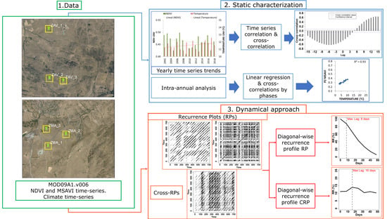
2. Materials and Methods
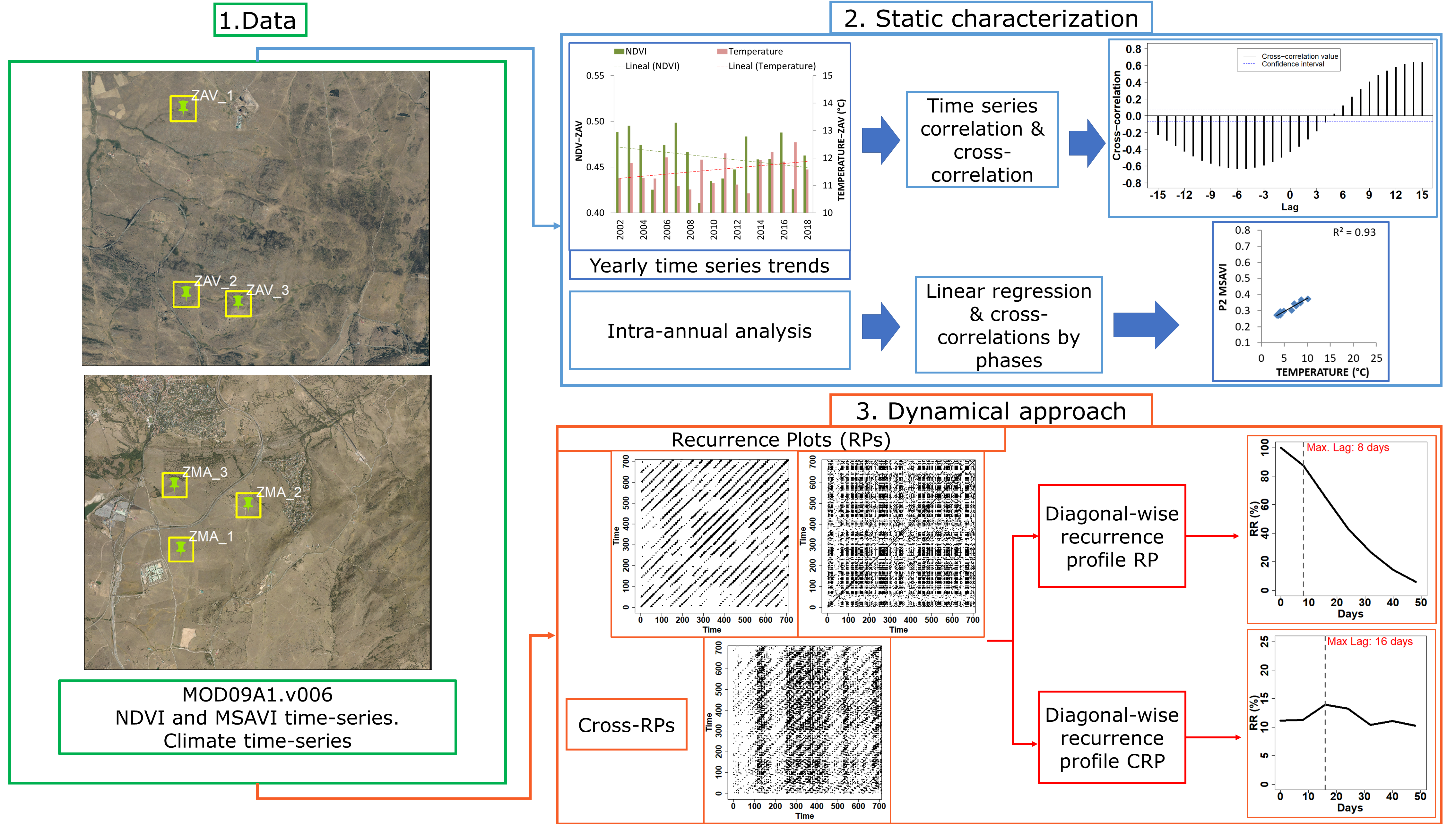
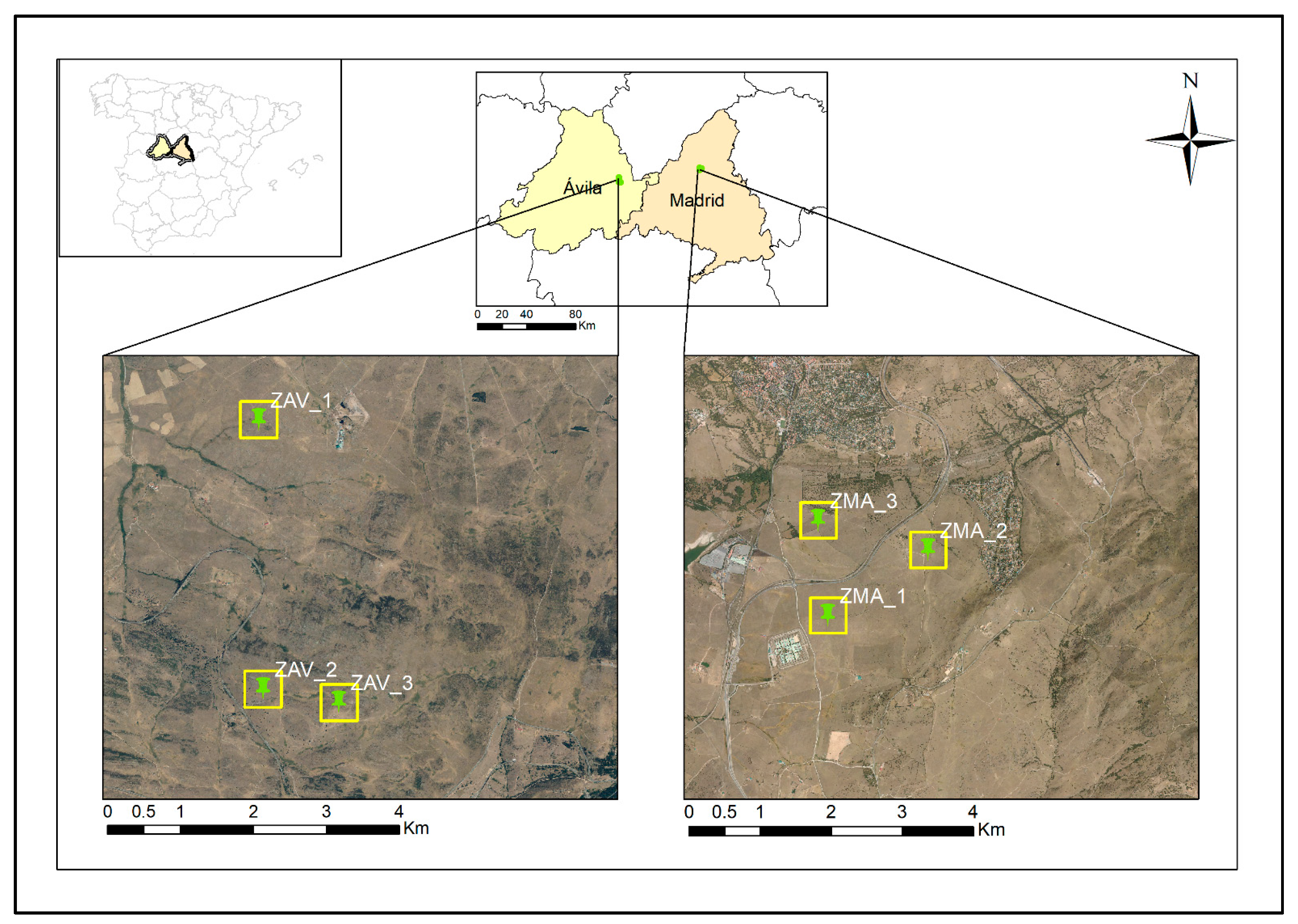
2.1. Study Area and Plots Selection
2.2. Acquisition of Satellite Data and VIs Calculations
2.3. Meteorological Variables
2.4. Inter-Annual and Intra-Annual Analysis
2.5. Time-Series and VIs Phase Cross-Correlations
2.6. Recurrence Plots and Recurrence Quantification Analysis
3. Results
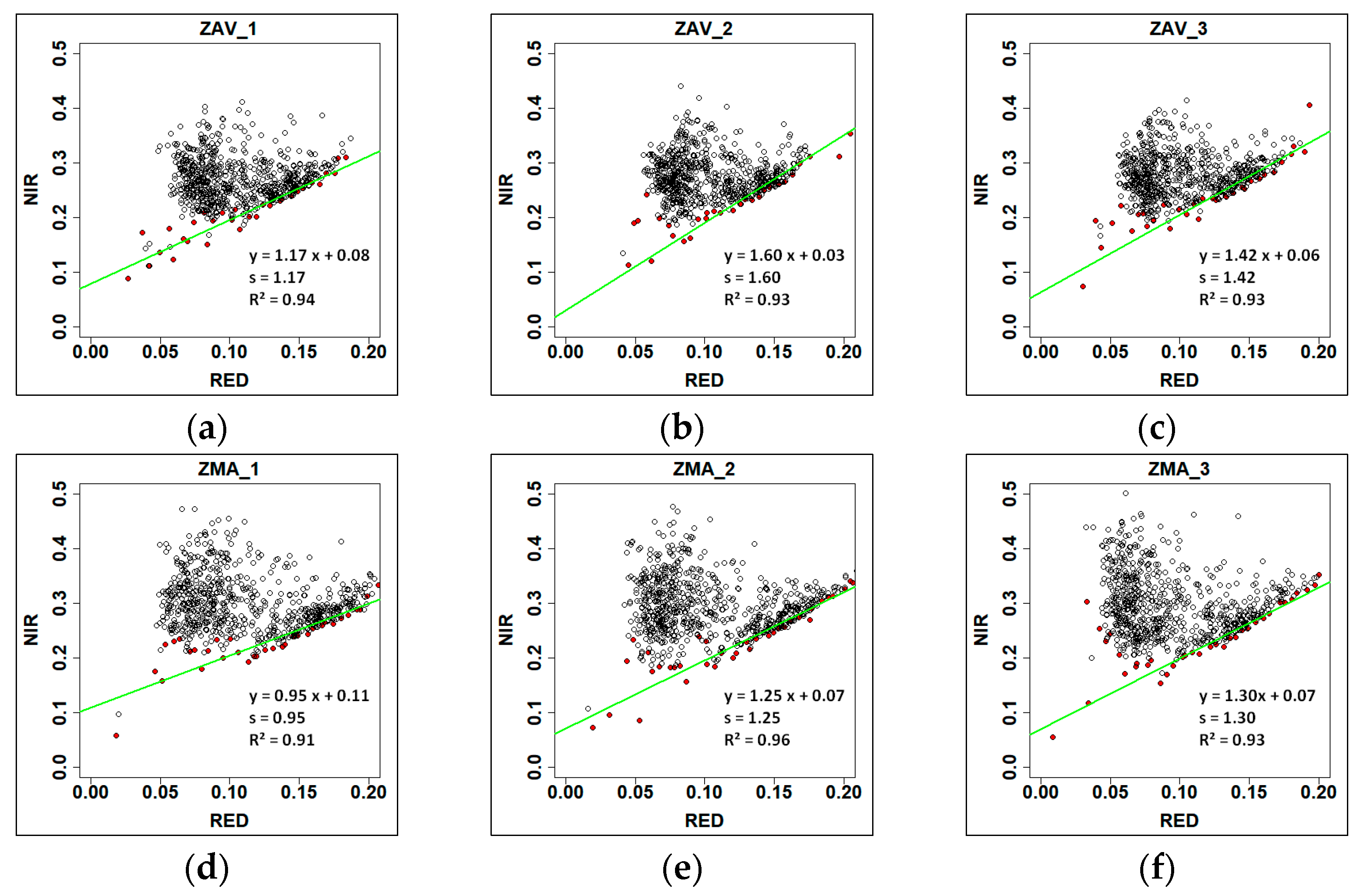
3.1. Soil Line Acquisition
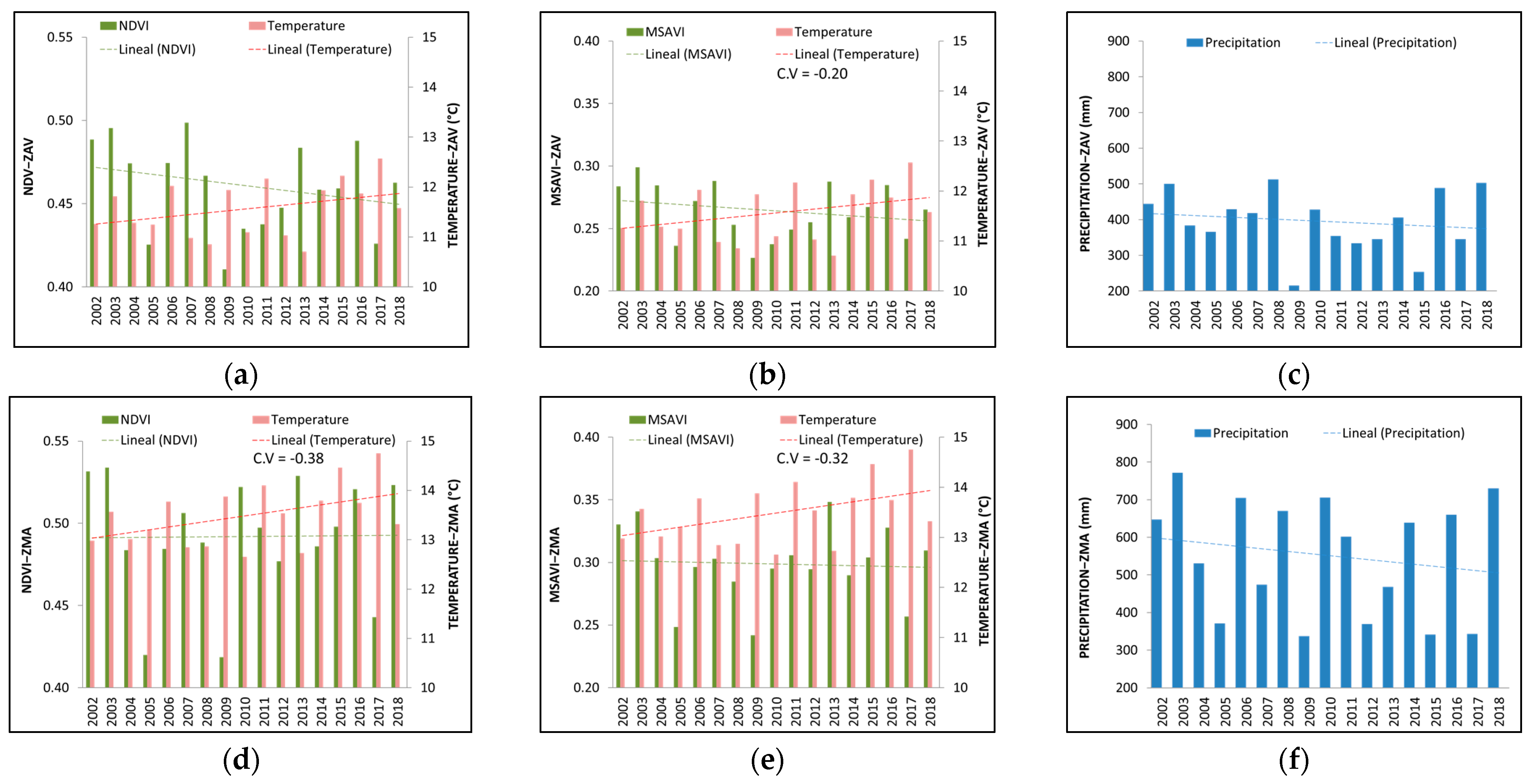
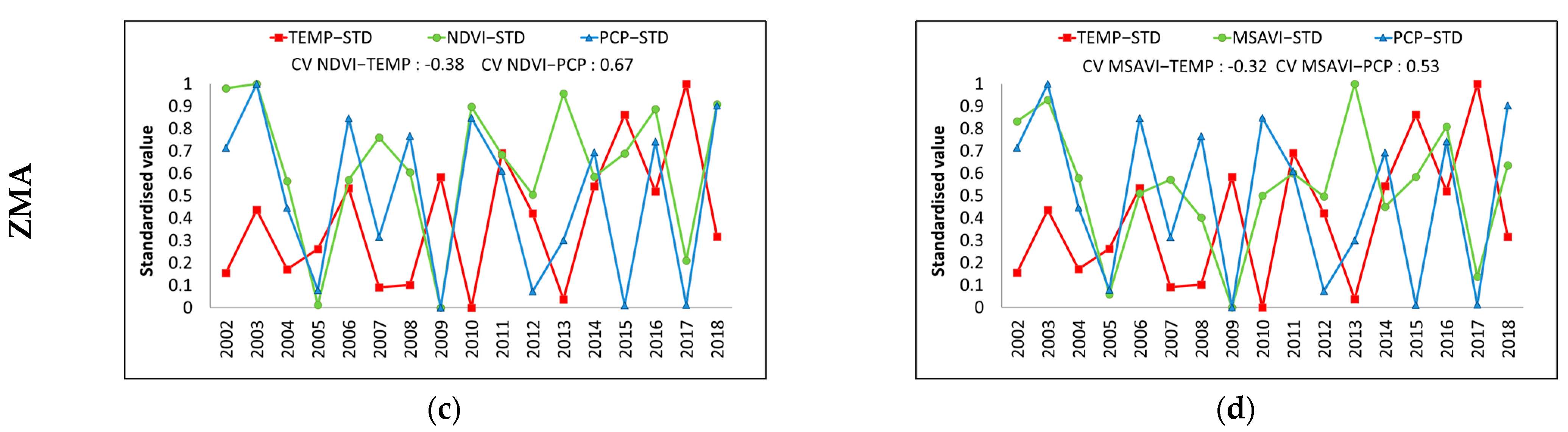
3.2. Inter-Annual Analysis
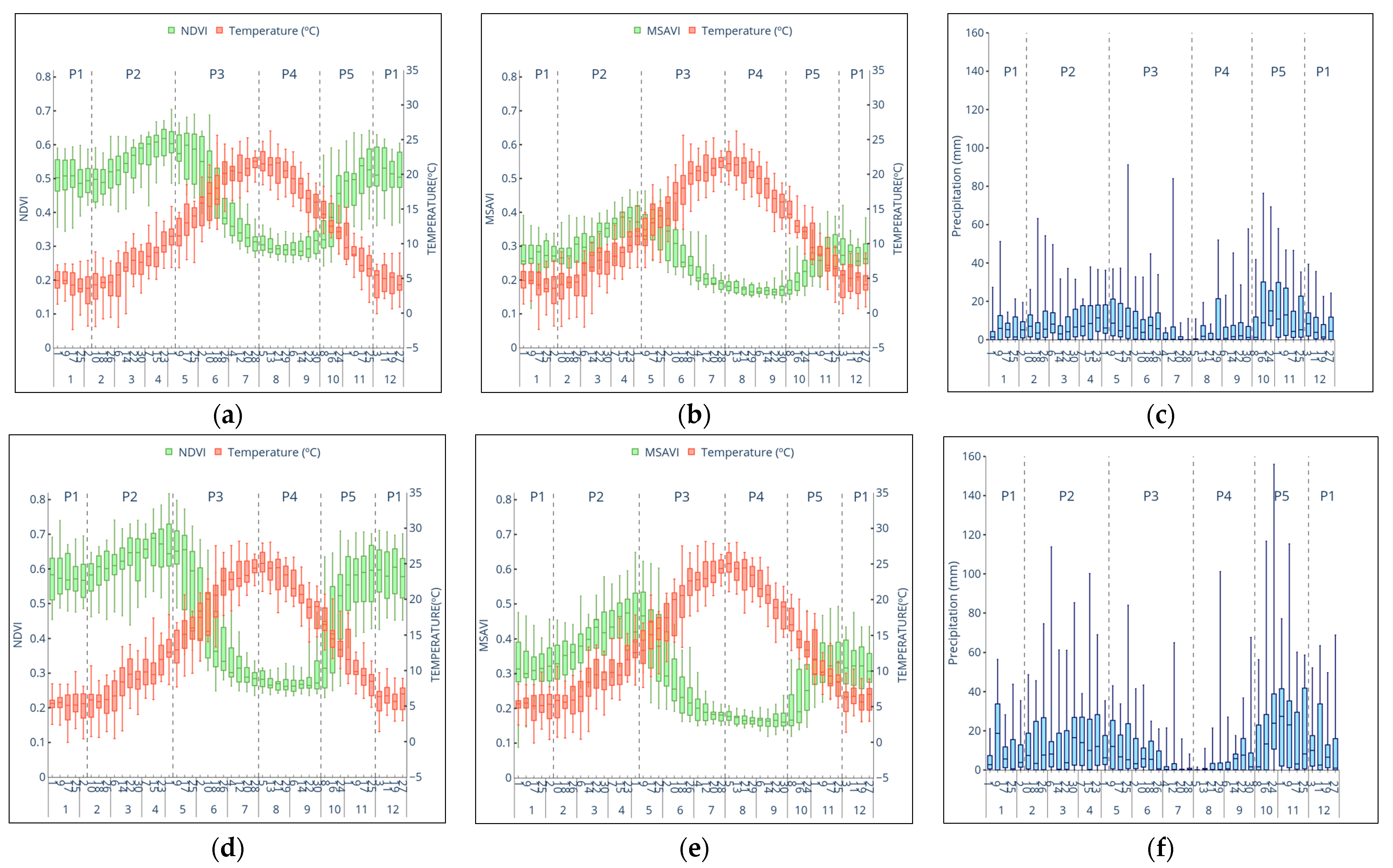
3.3. Intra-Annual Analysis
3.4. Time-Series Correlation
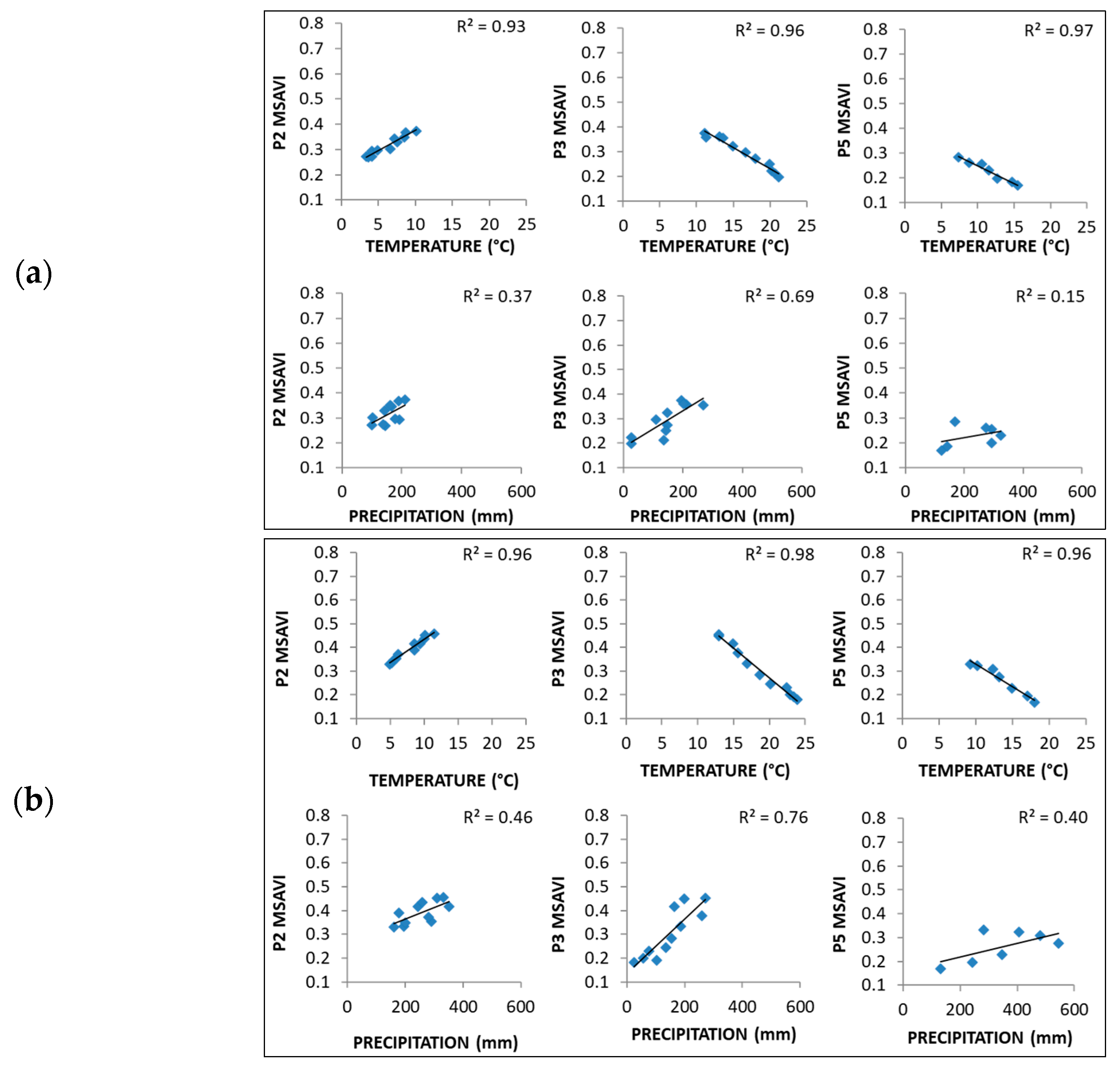
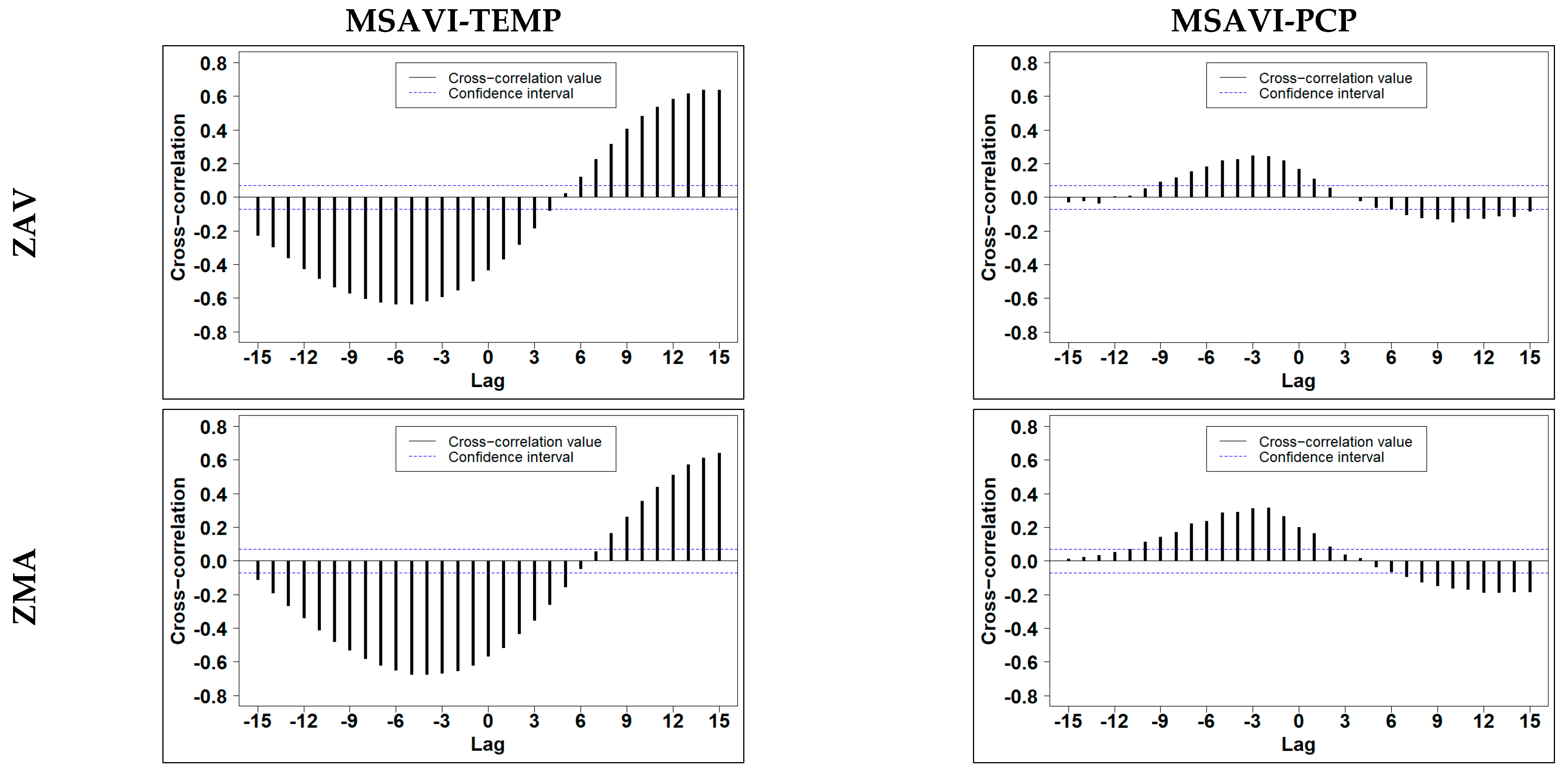
3.5. Correlation by Phase
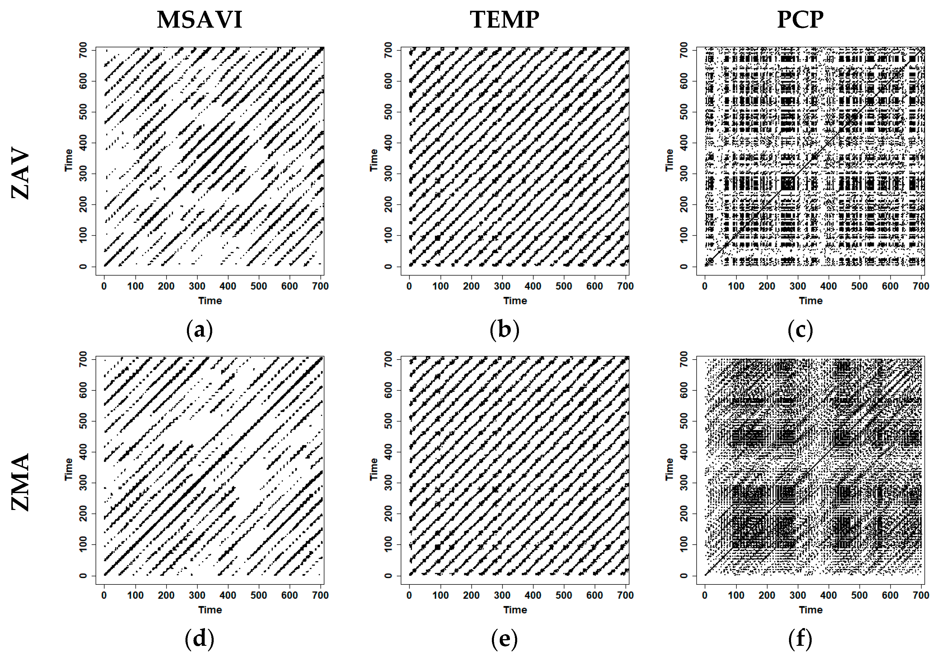
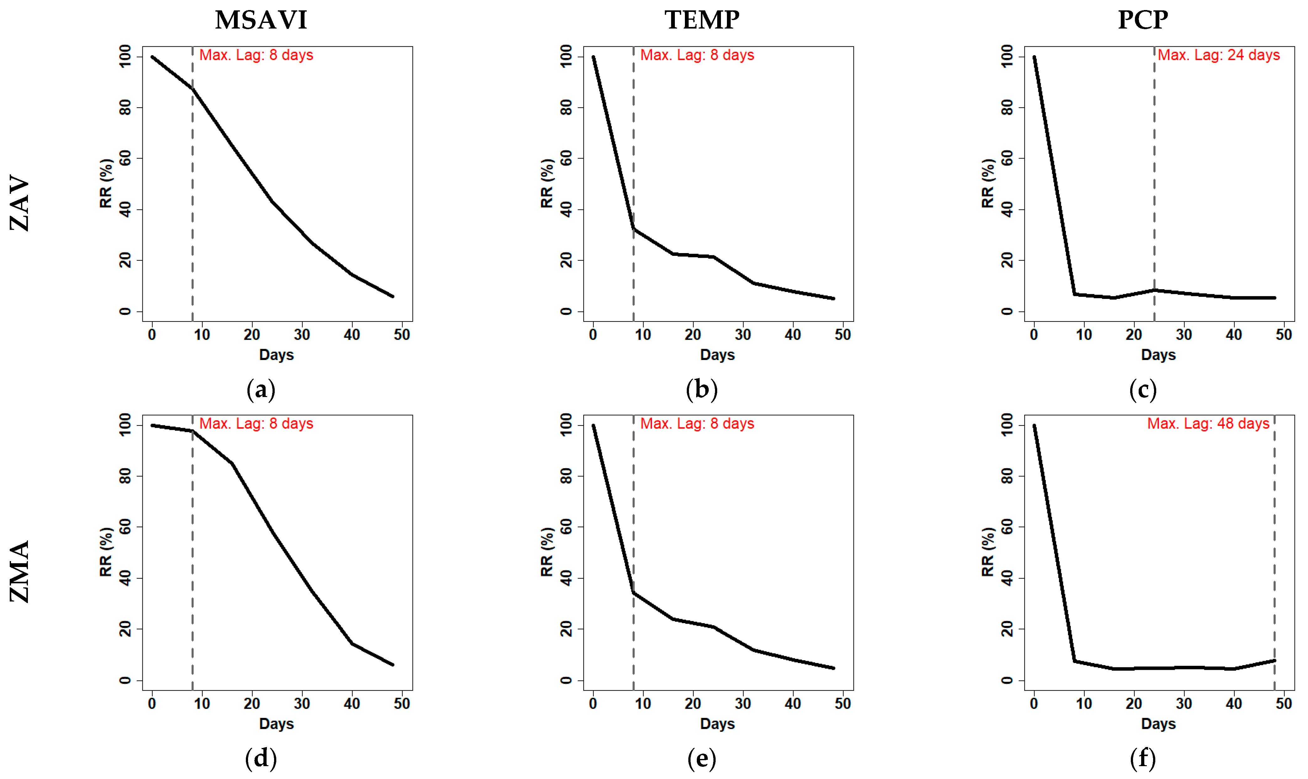
3.6. RPs Characterisation and Recurrence Diagonal Profile
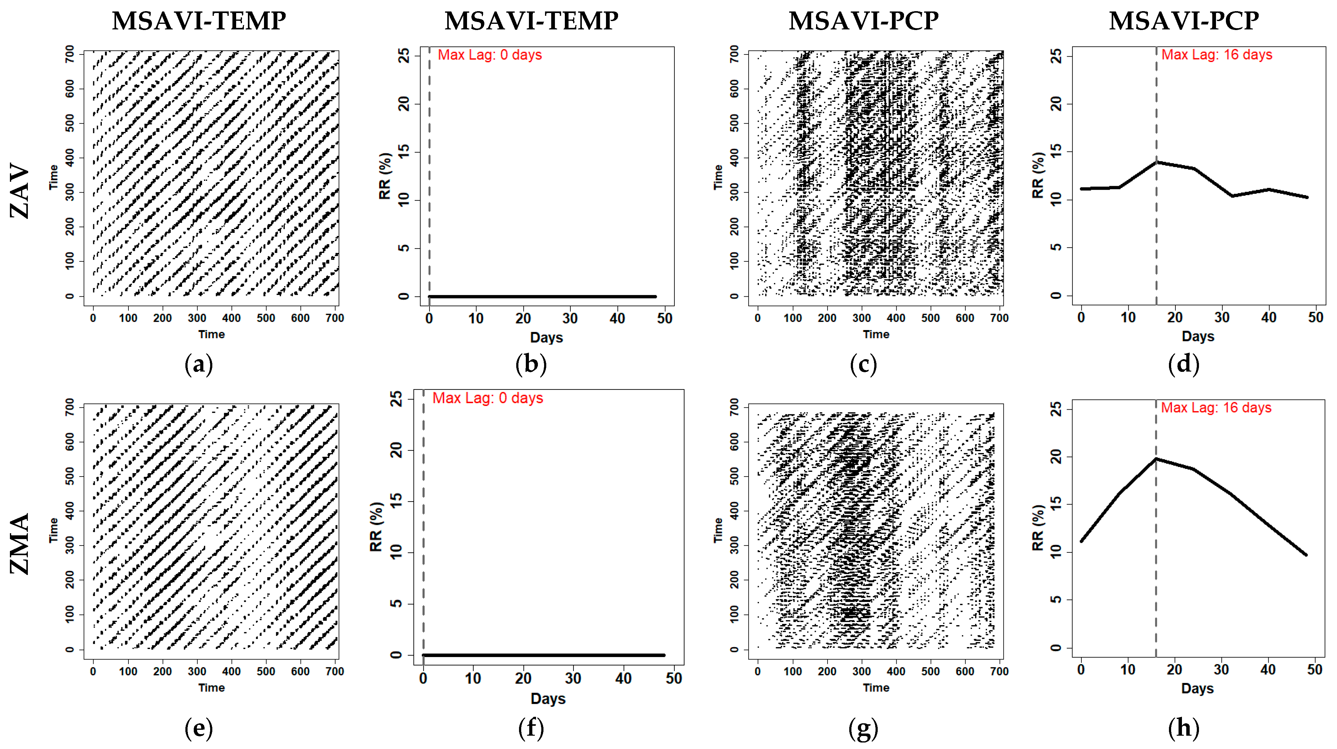
3.7. CRPs Characterisation and CRPs Diagonal Profile
3.8. Recurrence Quantification Analysis of RPs and CRPs
4. Discussion
5. Conclusions
Supplementary Materials
Author Contributions
Funding
Data Availability Statement
Conflicts of Interest
Appendix A
References
- Konings, A.G.; Williams, A.P.; Gentine, P. Sensitivity of grassland productivity to aridity controlled by stomatal and xylem regulation. Nat. Geosci. 2017, 10, 284–288. [Google Scholar] [CrossRef]
- Scheuring, I.; Riedi, R.H. Application of multifractals to the analysis of vegetation pattern. J. Veg. Sci. 1994, 5, 489–496. [Google Scholar] [CrossRef]
- Hobbs, R.J.; Yates, S.; Mooney, H.A. Long-term data reveal complex dynamics in grassland in relation to climate and disturbance. Ecol. Monogr. 2007, 77, 545–568. [Google Scholar] [CrossRef]
- Serrano, J.; Shahidian, S.; da Silva, J.M. Evaluation of normalised difference water index as a tool for monitoring pasture seasonal and inter-annual variability in a Mediterranean agro-silvo-pastoral system. Water 2019, 11, 62. [Google Scholar] [CrossRef]
- Li, B.; Tao, S.; Dawson, R.W. Relations between AVHRR NDVI and ecoclimatic parameters in China. Int. J. Remote Sens. 2002, 23, 989–999. [Google Scholar] [CrossRef]
- Wang, J.; Rich, P.M.; Price, K.P. Temporal responses of NDVI to precipitation and temperature in the central Great Plains, USA. Int. J. Remote Sens. 2003, 24, 2345–2364. [Google Scholar] [CrossRef]
- Cui, L.; Shi, J. Temporal and spatial response of vegetation NDVI to temperature and precipitation in eastern China. J. Geogr. Sci. 2010, 20, 163–176. [Google Scholar] [CrossRef]
- Gessner, U.; Naeimi, V.; Klein, I.; Kuenzer, C.; Klein, D.; Dech, S. The relationship between precipitation anomalies and satellite-derived vegetation activity in Central Asia. Glob. Planet. Chang. 2013, 110, 74–87. [Google Scholar] [CrossRef]
- Braswell, B.H.; Schimel, D.S.; Linder, E.; Moore, B. The Response of Global Terrestrial Ecosystems to Interannual Temperature Variability. Science 1997, 278, 870–873. [Google Scholar] [CrossRef]
- Piao, S.; Mohammat, A.; Fang, J.; Cai, Q.; Feng, J. NDVI-based increase in growth of temperate grasslands and its responses to climate changes in China. Glob. Environ. Chang. 2006, 16, 340–348. [Google Scholar] [CrossRef]
- Liu, Y.; Zha, Y.; Gao, J.; Ni, S. Assessment of grassland degradation near Lake Qinghai, West China, using Landsat TM and in situ reflectance spectra data. Int. J. Remote Sens. 2004, 25, 4177–4189. [Google Scholar] [CrossRef]
- Hively, W.D.; Lamb, B.T.; Daughtry, C.S.T.; Shermeyer, J.; McCarty, G.W.; Quemada, M. Mapping crop residue and tillage intensity using WorldView-3 satellite shortwave infrared residue indices. Remote Sens. 2018, 10, 1657. [Google Scholar] [CrossRef]
- Blanco, L.J.; Paruelo, J.M.; Oesterheld, M.; Biurrun, F.N. Spatial and temporal patterns of herbaceous primary production in semiarid shrublands: A remote sensing approach. J. Veg. Sci. 2016, 27, 716–727. [Google Scholar] [CrossRef]
- Steele-Dunne, S.C.; McNairn, H.; Monsivais-Huertero, A.; Judge, J.; Liu, P.W.; Papathanassiou, K. Radar Remote Sensing of Agricultural Canopies: A Review. IEEE J. Sel. Top. Appl. Earth Obs. Remote Sens. 2017, 10, 2249–2273. [Google Scholar] [CrossRef]
- Liu, S.; Gao, L.; Lei, Y.; Wang, M.; Hu, Q.; Ma, X.; Zhang, Y. SAR Speckle Removal Using Hybrid Frequency Modulations. IEEE Trans. Geosci. Remote Sens. 2020, 59, 3956–3966. [Google Scholar] [CrossRef]
- Das, A.; Agrawal, R.; Mohan, S. Topographic correction of ALOS-PALSAR images using InSAR-derived DEM. Geocarto Int. 2015, 30, 145–153. [Google Scholar] [CrossRef]
- Mao, D.; Wang, Z.; Luo, L.; Ren, C. Integrating AVHRR and MODIS data to monitor NDVI changes and their relationships with climatic parameters in Northeast China. Int. J. Appl. Earth Obs. Geoinf. 2012, 18, 528–536. [Google Scholar] [CrossRef]
- Guo, B.; Zhou, Y.; Wang, S.; Tao, H. The relationship between normalised difference vegetation index (NDVI) and climate factors in the semiarid region: A case study in Yalu Tsangpo River basin of Qinghai-Tibet Plateau. J. Mt. Sci. 2014, 11, 926–940. [Google Scholar] [CrossRef]
- Rouse, J.W.; Haas, R.H.; Schell, J.A.; Deering, D.W. Monitoring the vernal advancement and retrogradation (green wave effect) of natural vegetation. Progress Report RSC 1978-1. 1973, Volume 112. Available online: https://core.ac.uk/download/pdf/80640125.pdf (accessed on 30 April 2021).
- Huete, A.; Didan, K.; Miura, T.; Rodriguez, E.P.; Gao, X.; Ferreira, L.G. Overview of the radiometric and biophysical performance of the MODIS vegetation indices. Remote Sens. Environ. 2002, 83, 195–213. [Google Scholar] [CrossRef]
- Yang, L.; Wylie, B.K.; Tieszen, L.L.; Reed, B.C. An analysis of relationships among climate forcing and time-integrated NDVI of grasslands over the U.S. northern and central Great Plains. Remote Sens. Environ. 1998, 65, 25–37. [Google Scholar] [CrossRef]
- Jafari, R.; Bashari, H.; Tarkesh, M. Discriminating and monitoring rangeland condition classes with MODIS NDVI and EVI indices in Iranian arid and semiarid lands. Arid Land Res. Manag. 2017, 31, 94–110. [Google Scholar] [CrossRef]
- Yagci, A.L.; Di, L.; Deng, M. The influence of land cover-related changes on the NDVI-based satellite agricultural drought indices. In Proceedings of the 2014 IEEE Geoscience and Remote Sensing Symposium, Quebe, QC, Canada, 13–18 July 2014; pp. 2054–2057. [Google Scholar] [CrossRef]
- Fern, R.R.; Foxley, E.A.; Bruno, A.; Morrison, M.L. Suitability of NDVI and OSAVI as estimators of green biomass and coverage in a semiarid rangeland. Ecol. Indic. 2018, 94, 16–21. [Google Scholar] [CrossRef]
- Huete, A.R.; Jackson, R.D.; Post, D.F. Spectral response of a plant canopy with different soil backgrounds. Remote Sens. Environ. 1985, 17, 37–53. [Google Scholar] [CrossRef]
- Eisfelder, C.; Kuenzer, C.; Dech, S. Derivation of biomass information for semi-arid areas using remote-sensing data. Int. J. Remote Sens. 2012, 33, 2937–2984. [Google Scholar] [CrossRef]
- Ren, H.; Zhou, G.; Zhang, F. Using negative soil adjustment factor in soil-adjusted vegetation index (SAVI) for above-ground living biomass estimation in arid grasslands. Remote Sens. Environ. 2018, 209, 439–445. [Google Scholar] [CrossRef]
- Qi, J.; Chehbouni, A.; Huete, A.R.; Kerr, Y.H.; Sorooshian, S. A modified soil adjusted vegetation index. Remote Sens. Environ. 1994, 48, 119–126. [Google Scholar] [CrossRef]
- Jiang, Y.; Tao, J.; Huang, Y.; Zhu, J.; Tian, L.; Zhang, Y. The spatial pattern of grassland above-ground biomass on Xizang Plateau and its climatic controls. J. Plant. Ecol. 2013, 8, 30–40. [Google Scholar] [CrossRef]
- Li, G.; Wang, J.; Wang, Y.; Wei, H.; Ochir, A.; Davaasuren, D.; Chonokhuu, S.; Nasanbat, E. Spatial and temporal variations in grassland production from 2006 to 2015 in Mongolia along the China-Mongolia Railway. Sustainability 2019, 11, 2177. [Google Scholar] [CrossRef]
- Chamaille-Jammes, S.; Fritz, H.; Murindagomo, F. Spatial patterns of the NDVI-rainfall relationship at the seasonal and interannual time scales in an African savanna. Int. J. Remote Sens. 2006, 27, 5185–5200. [Google Scholar] [CrossRef]
- Ma, X.; Huete, A.; Yu, Q.; Coupe, N.R.; Davies, K.; Broich, M.; Ratana, P.; Beringer, J.; Hutley, L.B.; Cleverly, J.; et al. Spatial patterns and temporal dynamics in savanna vegetation phenology across the north australian tropical transect. Remote Sens. Environ. 2013, 139, 97–115. [Google Scholar] [CrossRef]
- Zhang, Y.; Wang, X.; Li, C.; Cai, Y.; Yang, Z.; Yi, Y. NDVI dynamics under changing meteorological factors in a shallow lake in future metropolitan, semiarid area in North China. Sci. Rep. 2018, 8, 1–13. [Google Scholar] [CrossRef]
- Chen, Z.; Wang, W.; Fu, J. Vegetation response to precipitation anomalies under different climatic and biogeographical conditions in China. Sci. Rep. 2020, 10, 1–16. [Google Scholar] [CrossRef]
- Cong, N.; Shen, M.; Yang, W.; Yang, Z.; Zhang, G.; Piao, S. Varying responses of vegetation activity to climate changes on the Tibetan Plateau grassland. Int. J. Biometeorol. 2017, 61, 1433–1444. [Google Scholar] [CrossRef]
- Wang, H.; Liu, D.; Lin, H.; Montenegro, A.; Zhu, X. NDVI and vegetation phenology dynamics under the influence of sunshine duration on the Tibetan plateau. Int. J. Climatol. 2015, 35, 687–698. [Google Scholar] [CrossRef]
- Shen, B.; Fang, S.; Li, G. Vegetation coverage changes and their response to meteorological variables from 2000 to 2009 in Naqu, Tibet, China. Can. J. Remote Sens. 2014, 40, 67–74. [Google Scholar] [CrossRef]
- Martínez, B.; Gilabert, M.A. Vegetation dynamics from NDVI time series analysis using the wavelet transform. Remote Sens. Environ. 2009, 113, 1823–1842. [Google Scholar] [CrossRef]
- Zhong, L.; Ma, Y.; Salama, M.S.; Su, Z. Assessment of vegetation dynamics and their response to variations in precipitation and temperature in the Tibetan Plateau. Clim. Chang. 2010, 103, 519–535. [Google Scholar] [CrossRef]
- Zhao, Z.; Liu, J.; Peng, J.; Li, S.; Wang, Y. Nonlinear features and complexity patterns of vegetation dynamics in the transition zone of North China. Ecol. Indic. 2015, 49, 237–246. [Google Scholar] [CrossRef]
- Eckmann, J.P.; Oliffson Kamphorst, O.; Ruelle, D. Recurrence plots of dynamical systems. Europhys. Lett. 1987, 4, 973–977. [Google Scholar] [CrossRef]
- Proulx, R.; Parrott, L.; Fahrig, L.; Currie, D.J. Long Time-Scale Recurrences in Ecology: Detecting Relationships Between Climate Dynamics and Biodiversity Along a Latitudinal Gradient. In Recurrence Quantification Analysis—Theory and Best Practices; Webber, C.L., Marwan, N., Eds.; Springer International Publishing: Cham, Germany, 2015; pp. 335–347. [Google Scholar]
- Marwan, N.; Carmen Romano, M.; Thiel, M.; Kurths, J. Recurrence plots for the analysis of complex systems. Phys. Rep. 2007, 438, 237–329. [Google Scholar] [CrossRef]
- Proulx, R.; Cöté, P.; Parrott, L. Use of recurrence analysis to measure the dynamical stability of a multi-species community model. Eur. Phys. J. Spec. Top. 2008, 164, 117–126. [Google Scholar] [CrossRef]
- Li, S.C.; Zhao, Z.Q.; Liu, F.Y. Identifying spatial pattern of NDVI series dynamics using recurrence quantification analysis. Eur. Phys. J. Spec. Top. 2008, 164, 127–139. [Google Scholar] [CrossRef]
- Zurlini, G.; Marwan, N.; Semeraro, T.; Jones, K.B.; Aretano, R.; Pasimeni, M.R.; Valente, D.; Mulder, C.; Petrosillo, I. Investigating landscape phase transitions in Mediterranean rangelands by recurrence analysis. Landsc. Ecol. 2018, 33, 1617–1631. [Google Scholar] [CrossRef]
- Semeraro, T.; Luvisi, A.; Lillo, A.O.; Aretano, R.; Buccolieri, R.; Marwan, N. Recurrence analysis of vegetation indices for highlighting the ecosystem response to drought events: An application to the amazon forest. Remote Sens. 2020, 12, 907. [Google Scholar] [CrossRef]
- LP DAAC. Land Processes Distributed Active Archive Center: Surface Reflectance 8-Day L3 Global 500 m, NASA and USGS. 2014. Available online: https://lpdaac.usgs.gov/products/mod09a1v006/ (accessed on 30 April 2021).
- Martín-Sotoca, J.J.; Saa-Requejo, A.; Moratiel, R.; Dalezios, N.; Faraslis, I.; Tarquis, A.M. Statistical analysis for satellite-index-based insurance to define damaged pasture thresholds. Nat. Hazards Earth Syst. Sci. 2019, 19, 1685–1702. [Google Scholar] [CrossRef]
- Xu, D.; Guo, X. A study of soil line simulation from landsat images in mixed grassland. Remote Sens. 2013, 5, 4533–4550. [Google Scholar] [CrossRef]
- Xu, M.; Eckstein, Y. Use of Weighted Least-Squares Method in Evaluation of the Relationship Between Dispersivity and Field Scale. Groundwater 1995, 33, 905–908. [Google Scholar] [CrossRef]
- Agencia Estatal de Meteorología AEMET OpenData. Available online: https://opendata.aemet.es/centrodedescargas/inicio (accessed on 24 May 2019).
- Tarquis, A.M.; Castellanos, M.T.; Cartagena, M.C.; Arce, A.; Ribas, F.; Cabello, M.J.; De Herrera, J.L.; Bird, N.R.A. Scale and space dependencies of soil nitrogen variability. Nonlinear Process. Geophys. 2017, 24, 77–87. [Google Scholar] [CrossRef]
- Chow, G.C. Tests of Equality Between Sets of Coefficients in Two Linear Regressions. Econom. J. Econom. Soc. 1960, 28, 591–605. [Google Scholar] [CrossRef]
- Coco, M.I.; Dale, R. Cross-recurrence quantification analysis of categorical and continuous time series: An R package. Front. Psychol. 2014, 5, 510. [Google Scholar] [CrossRef] [PubMed]
- Marwan, N. CRP Toolbox 5.22 (R32.4). Available online: http://tocsy.pik-potsdam.de/CRPtoolbox/ (accessed on 28 June 2019).
- Webber, C.L.; Zbilut, J. Recurrence quantification analysis of nonlinear dynamical systems. In Tutorials in Contemporary Nonlinear Methods for the Behavioral Sciences Web Book; 2005; pp. 26–94. Available online: http://www.nsf.gov/sbe/bcs/pac/nmbs/nmbs.jsp (accessed on 5 June 2019).
- Fraser, A.M.; Swinney, H.L. Independent coordinates for strange attractors from mutual information. Phys. Rev. A 1986, 33, 1134–1140. [Google Scholar] [CrossRef] [PubMed]
- Cao, L. Practical method for determining the minimum embedding dimension of a scalar time series. Phys. D Nonlinear Phenom. 1997, 110, 43–50. [Google Scholar] [CrossRef]
- Baret, F.; Jacquemoud, S.; Hanocq, J.F. About The soil line concept in remote sensing. Adv. Sp. Res. 1993, 13, 281–284. [Google Scholar] [CrossRef]
- Quemada, M.; Hively, W.D.; Daughtry, C.S.T.; Lamb, B.T.; Shermeyer, J. Improved crop residue cover estimates obtained by coupling spectral indices for residue and moisture. Remote Sens. Environ. 2018, 206, 33–44. [Google Scholar] [CrossRef]
- Chuai, X.W.; Huang, X.J.; Wang, W.J.; Bao, G. NDVI, temperature and precipitation changes and their relationships with different vegetation types during 1998–2007 in Inner Mongolia, China. Int. J. Climatol. 2013, 33, 1696–1706. [Google Scholar] [CrossRef]
- Hao, F.; Zhang, X.; Ouyang, W.; Skidmore, A.K.; Toxopeus, A.G. Vegetation NDVI Linked to Temperature and Precipitation in the Upper Catchments of Yellow River. Environ. Model. Assess. 2012, 17, 389–398. [Google Scholar] [CrossRef]
- Vicente-Serrano, S.M.; Tomas-Burguera, M.; Beguería, S.; Reig, F.; Latorre, B.; Peña-Gallardo, M.; Luna, M.Y.; Morata, A.; González-Hidalgo, J.C. A high resolution dataset of drought indices for Spain. Data 2017, 2, 22. [Google Scholar] [CrossRef]
- Estrela, T.; Vargas, E. Drought Management Plans in the European Union. The Case of Spain. Water Resour. Manag. 2012, 26, 1537–1553. [Google Scholar] [CrossRef]
- Pang, G.; Wang, X.; Yang, M. Using the NDVI to identify variations in, and responses of, vegetation to climate change on the Tibetan Plateau from 1982 to 2012. Quat. Int. 2017, 444, 87–96. [Google Scholar] [CrossRef]
- Xu, Y.; Yang, J.; Chen, Y. NDVI-based vegetation responses to climate change in an arid area of China. Theor. Appl. Climatol. 2016, 126, 213–222. [Google Scholar] [CrossRef]
- Liu, Y.; Li, Y.; Li, S.; Motesharrei, S. Spatial and temporal patterns of global NDVI trends: Correlations with climate and human factors. Remote Sens. 2015, 7, 13233–13250. [Google Scholar] [CrossRef]
- Huete, A.R. Soil influences in remotely sensed vegetation-canopy spectra. In Theory and Applications of Optical Remote Sensing; Asrar, G., Ed.; Wiley: New York, NY, USA, 1989. [Google Scholar]
- Sun, J.; Qin, X. Precipitation and temperature regulate the seasonal changes of NDVI across the Tibetan Plateau. Environ. Earth Sci. 2016, 75, 291. [Google Scholar] [CrossRef]
- Suzuki, R.; Masuda, K.G.; Dye, D. Interannual covariability between actual evapotranspiration and PAL and GIMMS NDVIs of northern Asia. Remote Sens. Environ. 2007, 106, 387–398. [Google Scholar] [CrossRef]
- Viola, F.; Daly, E.; Vico, G.; Cannarozzo, M.; Porporato, A. Transient soil-moisture dynamics and climate change in Mediterranean ecosystems. Water Resour. Res. 2008, 44. [Google Scholar] [CrossRef]
- Grant, K.; Kreyling, J.; Dienstbach, L.F.H.; Beierkuhnlein, C.; Jentsch, A. Water stress due to increased intra-annual precipitation variability reduced forage yield but raised forage quality of a temperate grassland. Agric. Ecosyst. Environ. 2014, 186, 11–22. [Google Scholar] [CrossRef]
- Fu, B.; Burgher, I. Riparian vegetation NDVI dynamics and its relationship with climate, surface water and groundwater. J. Arid Environ. 2015, 113, 59–68. [Google Scholar] [CrossRef]
- Sala, O.E.; Parton, W.J.; Joyce, L.A.; Lauenroth, W.K. Primary Production of the Central Grassland Region of the United States. Ecology 1988, 69, 40–45. [Google Scholar] [CrossRef]
- Olmos-Trujillo, E.; González-Trinidad, J.; Júnez-Ferreira, H.; Pacheco-Guerrero, A.; Bautista-Capetillo, C.; Avila-Sandoval, C.; Galván-Tejada, E. Spatio-temporal response of vegetation indices to rainfall and temperature in a semiarid region. Sustainbility 2020, 12, 1939. [Google Scholar] [CrossRef]
- Cao, X.M.; Chen, X.; Bao, A.M.; Wang, Q. Response of vegetation to temperature and precipitation in Xinjiang during the period of 1998–2009. J. Arid Land 2011, 3, 94–103. [Google Scholar] [CrossRef]
- Guo, L.; Wu, S.; Zhao, D.; Yin, Y.; Leng, G.; Zhang, Q. NDVI-Based Vegetation Change in Inner Mongolia from 1982 to 2006 and Its Relationship to Climate at the Biome Scale. Adv. Meteorol. 2014, 2014. [Google Scholar] [CrossRef]
- Gong, Z.; Kawamura, K.; Ishikawa, N.; Goto, M.; Wulan, T.; Alateng, D.; Yin, T.; Ito, Y. MODIS normalised difference vegetation index (NDVI) and vegetation phenology dynamics in the Inner Mongolia grassland. Solid Earth 2015, 6, 1185–1194. [Google Scholar] [CrossRef]
- Helman, D.; Lensky, I.M.; Tessler, N.; Osem, Y. A phenology-based method for monitoring woody and herbaceous vegetation in mediterranean forests from NDVI time series. Remote Sens. 2015, 7, 12314–12335. [Google Scholar] [CrossRef]
- Ramos, M.C. Rainfall distribution patterns and their change over time in a Mediterranean area. Theor. Appl. Climatol. 2001, 69, 163–170. [Google Scholar] [CrossRef]
- Meroni, M.; Rembold, F.; Verstraete, M.M.; Gommes, R.; Schucknecht, A.; Beye, G. Investigating the relationship between the inter-annual variability of satellite-derived vegetation phenology and a proxy of biomass production in the Sahel. Remote Sens. 2014, 6, 5868–5884. [Google Scholar] [CrossRef]
- Proulx, R.; Parrott, L. Structural complexity in digital images as an ecological indicator for monitoring forest dynamics across scale, space and time. Ecol. Indic. 2009, 9, 1248–1256. [Google Scholar] [CrossRef]
- Storch, D.; Gaston, K.J. Untangling ecological complexity on different scales of space and time. Basic Appl. Ecol. 2004, 5, 389–400. [Google Scholar] [CrossRef]
- Belaire-Franch, J.; Contreras, D.; Tordera-Lledó, L. Assessing nonlinear structures in real exchange rates using recurrence plot strategies. Phys. D Nonlinear Phenom. 2002, 171, 249–264. [Google Scholar] [CrossRef]
- Donner, R.V.; Zou, Y.; Donges, J.F.; Marwan, N.; Kurths, J. Recurrence networks—A novel paradigm for nonlinear time series analysis. New J. Phys. 2010, 12, 233025. [Google Scholar] [CrossRef]
- Marwan, N.; Kurths, J.; Foerster, S. Analysing spatially extended high-dimensional dynamics by recurrence plots. Phys. Lett. A 2015, 379, 894–900. [Google Scholar] [CrossRef]
- Richard, Y.; Poccard, I. A statistical study of NDVI sensitivity to seasonal and interannual rainfall variations in Southern Africa. Int. J. Remote Sens. 1998, 19, 2907–2920. [Google Scholar] [CrossRef]
- Zhao, J.; Huang, S.; Huang, Q.; Wang, H.; Leng, G.; Fang, W. Time-lagged response of vegetation dynamics to climatic and teleconnection factors. Catena 2020, 189, 104474. [Google Scholar] [CrossRef]
- Beckage, B.; Gross, L.J.; Kauffman, S. The limits to prediction in ecological systems. Ecosphere 2011, 2, 1–12. [Google Scholar] [CrossRef]
- Marwan, N.; Wessel, N.; Meyerfeldt, U.; Schirdewan, A.; Kurths, J. Recurrence-plot-based measures of complexity and their application to heart-rate-variability data. Phys. Rev. E 2002, 66, 026702. [Google Scholar] [CrossRef] [PubMed]


| Variable | ZAV | ZMA |
|---|---|---|
| Slope (%) | 4.2 (±1.10) | 4.7 (±1.60) |
| Height (m) | 1290 (±70) | 958 (±30) |
| Silt (%) | 20 (±2.00) | 18 (±1.00) |
| Sand (%) | 60 (±2.00) | 76 (±1.00) |
| Clay (%) | 20 (±2.00) | 6 (±1.00) |
| Bulk Density (g/cm3) | 1.3 (±0.10) | 1.6 (±0.10) |
| pH | 6.5 (±0.30) | 5.6 (±0.20) |
| Organic Matter (%) | 3.8 (±0.20) | 3.0 (±0.10) |
| Water Holding Capacity (%) | 14.4 (±1.00) | 11.1 (±1.00) |
| Precipitation (mm) | 400 (±150.00) | 560 (±80.00) |
| Temperature (°C) | 11.6 (±0.60) | 13.6 (±0.60) |
| Code Phase | Initial Date | Final Date | Months Implied | Seasons Implied | VIs Trend |
|---|---|---|---|---|---|
| P1 | 25 November | 25 January | November-December-January | Autumn–Winter | Constant |
| P2 | 2 February | 23 April | February-March-April | Winter–Spring | Increasing |
| P3 | 1 May | 20 June | May-June | Spring–Summer | Decreasing |
| P4 | 28 July | 22 September | July-August-September | Summer–Autumn | Constant |
| P5 | 30 September | 17 November | September-October-November | Autumn | Increasing |
| Zone | CR | PCR | ||
|---|---|---|---|---|
| TEMP | PCP | TEMP | PCP | |
| ZAV | −0.435 ** | 0.165 ** | −0.571 ** | 0.199 ** |
| ZMA | −0.572 ** | 0.199 ** | −0.504 ** | 0.074 ** |
| CR | PCR | ||||
|---|---|---|---|---|---|
| PHASE | MSAVI xTEMP | MSAVI x PCP | MSAVI x TEMP | MSAVI x PCP | |
| ZAV | P1 | 0.130 | 0.046 | 0.173* | 0.008 |
| P2 | 0.489 ** | 0.066 | −0.027 | 0.180 * | |
| P3 | −0.714 ** | 0.283 ** | −0.095 | −0.003 | |
| P4 | 0.270 ** | −0.037 | −0.130 | 0.106 | |
| P5 | −0.550 ** | 0.216 * | 0.072 | −0.052 | |
| ZMA | P1 | 0.101 | 0.023 | 0.144 | 0.015 |
| P2 | 0.428 ** | 0.042 | 0.026 | 0.125 | |
| P3 | −0.763 ** | 0.359 ** | −0.007 | −0.053 | |
| P4 | 0.248 ** | 0.029 | 0.007 | 0.135 | |
| P5 | −0.594 ** | 0.160 | 0.040 | −0.157 | |
| Time Lag (ℓ) | |||||||||
|---|---|---|---|---|---|---|---|---|---|
| Phase | Param. | 0 | 1 | 2 | 3 | 4 | 5 | 6 | |
| ZAV | P2 | TEMP | 0.492 | 0.451 | 0.418 | 0.333 | 0.271 | 0.198 | 0.041 |
| PCP | 0.067 | 0.039 | 0.074 | 0.133 | −0.031 | −0.003 | 0.079 | ||
| P3 | TEMP | −0.714 | −0.739 | −0.741 | −0.726 | −0.714 | −0.681 | −0.629 | |
| PCP | 0.283 | 0.312 | 0.378 | 0.243 | 0.256 | 0.186 | 0.064 | ||
| P5 | TEMP | −0.550 | −0.553 | −0.575 | −0.584 | −0.605 | −0.613 | −0.561 | |
| PCP | 0.216 | 0.359 | 0.396 | 0.424 | 0.235 | 0.214 | 0.241 | ||
| ZMA | P2 | TEMP | 0.422 | 0.308 | 0.259 | 0.233 | 0.169 | 0.109 | 0.029 |
| PCP | 0.032 | 0.088 | 0.186 | 0.221 | 0.156 | 0.102 | 0.093 | ||
| P3 | TEMP | −0.763 | −0.757 | −0.717 | −0.699 | −0.695 | −0.697 | −0.637 | |
| PCP | 0.359 | 0.396 | 0.381 | 0.321 | 0.357 | 0.309 | 0.230 | ||
| P5 | TEMP | −0.594 | −0.600 | −0.625 | −0.602 | −0.603 | −0.581 | −0.512 | |
| PCP | 0.159 | 0.297 | 0.393 | 0.397 | 0.293 | 0.275 | 0.304 | ||
| Zone | RPs | m | τ | RR (%) | |
|---|---|---|---|---|---|
| ZAV | MSAVI | 6 | 9 | 20.91 | 4.99 |
| TEMP | 2 | 11 | 8.76 | 4.99 | |
| PCP | 2 | 3 | 1.35 | 4.97 | |
| ZMA | MSAVI | 8 | 11 | 26.32 | 4.99 |
| TEMP | 2 | 11 | 9.00 | 4.99 | |
| PCP | 10 | 9 | 13.25 | 5.00 |
| Zone | CRPs | m | τ | RR (%) | |
|---|---|---|---|---|---|
| ZAV | MSAVI-TEMP | 6 | 11 | 23.04 | 5.00 |
| MSAVI-PCP | 6 | 11 | 17.27 | 5.00 | |
| ZMA | MSAVI-TEMP | 8 | 11 | 25.60 | 5.00 |
| MSAVI-PCP | 10 | 11 | 23.74 | 5.00 |
| Zone | RPs and CRPs | RR (%) | DET (%) | LT | ENTR | LAM (%) | TT |
|---|---|---|---|---|---|---|---|
| ZAV | MSAVI | 4.99 | 73.20 | 3.40 | 1.57 | 82.66 | 3.55 |
| TEMP | 4.99 | 40.26 | 2.31 | 0.72 | 52.89 | 2.49 | |
| PCP | 4.97 | 14.65 | 2.10 | 0.32 | 33.72 | 2.35 | |
| MSAVI-TEMP | 5.00 | 63.75 | 2.88 | 1.29 | 75.30 | 3.62 | |
| MSAVI-PCP | 5.00 | 19.25 | 2.17 | 0.47 | 23.08 | 2.27 | |
| ZMA | MSAVI | 4.99 | 78.42 | 4.17 | 1.80 | 86.13 | 3.88 |
| TEMP | 4.99 | 42.02 | 2.35 | 0.76 | 54.35 | 2.60 | |
| PCP | 5.00 | 6.57 | 2.03 | 0.14 | 20.72 | 2.11 | |
| MSAVI-TEMP | 5.00 | 69.06 | 3.21 | 1.50 | 76.59 | 3.75 | |
| MSAVI-PCP | 5.00 | 25.70 | 2.26 | 0.64 | 29.23 | 2.29 |
Publisher’s Note: MDPI stays neutral with regard to jurisdictional claims in published maps and institutional affiliations. |
© 2021 by the authors. Licensee MDPI, Basel, Switzerland. This article is an open access article distributed under the terms and conditions of the Creative Commons Attribution (CC BY) license (https://creativecommons.org/licenses/by/4.0/).
Share and Cite
Almeida-Ñauñay, A.F.; Benito, R.M.; Quemada, M.; Losada, J.C.; Tarquis, A.M. The Vegetation–Climate System Complexity through Recurrence Analysis. Entropy 2021, 23, 559. https://doi.org/10.3390/e23050559
Almeida-Ñauñay AF, Benito RM, Quemada M, Losada JC, Tarquis AM. The Vegetation–Climate System Complexity through Recurrence Analysis. Entropy. 2021; 23(5):559. https://doi.org/10.3390/e23050559
Chicago/Turabian StyleAlmeida-Ñauñay, Andrés F., Rosa María Benito, Miguel Quemada, Juan Carlos Losada, and Ana M. Tarquis. 2021. "The Vegetation–Climate System Complexity through Recurrence Analysis" Entropy 23, no. 5: 559. https://doi.org/10.3390/e23050559
APA StyleAlmeida-Ñauñay, A. F., Benito, R. M., Quemada, M., Losada, J. C., & Tarquis, A. M. (2021). The Vegetation–Climate System Complexity through Recurrence Analysis. Entropy, 23(5), 559. https://doi.org/10.3390/e23050559