1. Introduction
Network science focuses on the study of complex networks such as telecommunication, computer, biological, cognitive, and social networks. A network consists of nodes and links. The topological structure, which explores how nodes are connected in the system, has been investigated with great interest [
1,
2,
3]. Network researchers have examined foundational network topologies using various network-related quantities such as the degree distribution, clustering coefficient, and average path length. Most networks are dynamic, so accordingly, network-related quantities also change over time. Studying the evolution of these network quantities could provide insight into the behavior of individuals expressed by nodes and the change of topological properties of the network. The evolution of a network has been studied from various perspectives, e.g., the community [
4,
5], rich-get-richer [
1], node heterogeneity [
2,
6], and link persistence [
3].
The degree of a node is the number of links connected to a node. The degree distribution of a network,
, tells us the probability of degree
k that a randomly chosen node will have. One challenge in studying network science is to develop simplified measures that capture the network structure. The degree distribution is one of such measures that help to find influential nodes in the system. Many attempts have been made to study the degree distribution using Poisson, exponential, and power-law distributions. In particular, the analysis of the power-law degree distribution has been considered as one of the basic steps, and networks that have power-law degree distributions are often referred to as
scale-free networks. We can frequently observe power-law degree distributions in collaboration, World Wide Web, protein–protein interactions, and semantic networks [
7,
8,
9,
10]. The emergence of hubs (highly connected nodes) is a consequence of a scale-free property of networks. A rich-get-richer mechanism, also called a popularity effect [
11], has been known to produce power-law degree distributions and hubs [
1,
6].
Many dynamic network models have been developed to explain the power-law degree distribution in real networks. The most widely known dynamic model for the power-law degree distribution is the rich-get-richer generative model in Barabasi and Albert (1999) [
1], called the BA model. They employ the preferential attachment mechanism in which nodes with more neighbors tend to receive more links from other nodes. Specifically, the algorithm of the BA model has the following parts with the parameter
m that controls the number of links over time:
Growth: At each time point, a node enters the network. Then the node tries to connect with m nodes in the network.
Preferential attachment: The newly entered node connects with node i with probability proportional to the degree of node i.
The BA model yields a power-law degree distribution with exponent 3, i.e.,
. The exact form, given by Bollobas et al. in [
12], is:
There are many variant models to cover a broad range of power-law exponents [
13,
14,
15], degree correlations [
16], accelerating growth [
17,
18,
19], and node heterogeneity [
6,
20,
21]. Another model for generating the power-law degree distribution is a copying network model presented in Kumar et al. (2000) [
22]. In this model, newly entered nodes randomly select some existing nodes and copy some of the links.
The power-law distribution has the form of
, which can be expressed as
. Therefore, a straight line of
plot on
(log-log plot) can be an indication of a power-law relationship, and its slope is a power-law exponent. In real networks, however, the degree distribution does not have a shape of a straight line in the entire range. There are many empirical distributions where the power-law behavior is not observed in the range of small degrees. Many variants of the power-law distribution are developed to address this issue, such as generalized power-law distributions [
23,
24], composite distributions with threshold [
25,
26], and power-law distributions with an exponential cutoff [
27,
28]. However, these methods do not consider the essential foundation of the power-law. According to the BA model and its variants, the power-law nature is an inherent property exhibited from the preferential attachment rule. The model presented in this paper preserves the power-law nature to avoid manual modifications of the power-law distribution function, given by
.
Note that the BA model has a parameter
m. Jordan (2006) [
29] relieved the constant
m condition that, at each time, the number
M of connections can change over time according to the distribution of
M. The degree distribution turned out to be
We note the following statistical property.
Theorem 1. Suppose that M has a finite support, . Then the degree distribution of Jordan’s model can be expressed as a mixture distribution, given bywhere is a mixture weight corresponding to the mth mixture component in Equation (1), . Proof. Note that we can rewrite
and
as
from Equations (
1) and (
2). Then, we have
by
. □
Theorem 1 suggests that the degree distribution might be expressed as a mixture distribution. For example, we consider a network where a new node connects to one or two existing nodes, with probabilities
and
. Then we have the following degree distribution in a mixture form of the two BA model’s distributions with different
m,
Inspired by this property, we consider a mixture model as an explanation of the deviation from the power-law in the range of small degrees.
Moreover, many studies have considered the degree as a continuous variable using continuity assumptions [
30,
31]. This approach may mislead researchers since the degree is discrete-valued. Therefore, a discrete power-law distribution, called a truncated zeta distribution, is used in this paper.
In this study, we propose a mixture model of truncated zeta distributions for the analysis of degree distributions. The proposed model covers the entire range of the degree distribution through a mixture of truncated zeta distributions while maintaining the scale-free nature of a network. We can characterize the degree distribution more accurately through the discrete version of the power-law distribution. In addition, we present the maximum likelihood estimation algorithm along with a model selection method. A simulation study examines the validity of the proposed estimation procedure. In addition, real collaboration networks are investigated with the proposed model to describe the characteristics of the degree distribution.
We focus on analyzing actual scientific collaboration networks and have made significant advancements compared to the previous work in Jung and Phoa (2020) [
32]. The major improvements are as follows:
We detected some inconsistency in the scientific collaboration data. For example, “Smith, James,” “Smith, John,” and “Smith, Jacob” are all stated as “Smith, J” before 2007. Hence, we change the period of data to avoid the author name inconsistency for accurate inferences.
Moreover, a more elaborate analysis of the real data is conducted with noteworthy interpretations.
The validity of the presented algorithm is addressed with Monte Carlo simulations.
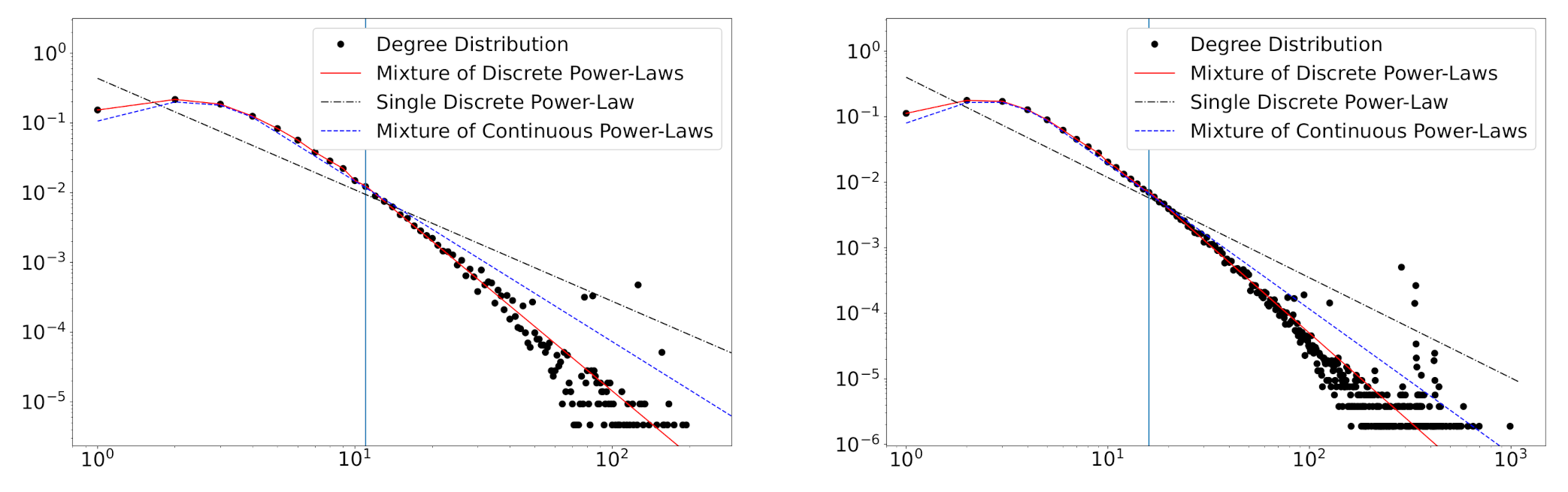
Extensive comparison studies are performed to show the superiority of the proposed model. We compared the proposed model with generalized Pareto models as well as base models that lack discreteness or mixture nature.
We provide more detailed explanations throughout the paper.
The rest of the paper is organized as follows. The continuous and discrete power-law distributions are defined in
Section 2, and the proposed mixture model of truncated zeta distributions is defined in
Section 3.
Section 4 presents the estimation method of the mixture model, and the validity of the estimation procedure is demonstrated in
Section 5. In
Section 6, we analyze the scientific collaboration network by applying the proposed mixture model with interpretations.
Section 7 concludes the paper.
3. Truncated Zeta Mixture Model
We consider the finite mixture model of truncated zeta distributions by fixing the power-law exponent
for mixture components while varying minimum values to produce a mixture of truncated zeta distributions. The probability mass function is represented as
where
is the pmf of
, and
L is the number of mixture components. Mixture weights
In this paper, we assume that the minimum value
l is equal to 1, but it can be modified according to the data. The tail of most real networks follows the power-law distribution, and Equation (
7) has the exact power-law behavior for sufficiently large degrees.
Theorem 2. For k larger than or equal to L, the truncated zeta mixture distribution in Equation (7) has the exact power-law relationship, given by Proof. By using the pmf of
, we can write
Since the term inside the bracket is independent with k, the pmf of the mixture is proportional to . □
Mixture models may suffer from the non-identifiability issue even for finite mixtures. The following theorem proves that the proposed truncated zeta mixture model is identifiable.
Theorem 3. The mixture distribution Equation (7) is identifiable with respect to α, L, and w. Proof. Let
and
be the mixture distributions of
,
,
and
,
,
, respectively. Suppose that
and
are identical, i.e.,
for all
. Further, we define the slope function
of the log-log degree distribution, given by
The equality of the two mixture distributions give the identical slope function, for all . We then have for the sufficiently large k. Therefore, we obtain . The number of mixture components L is the largest integer k such that , and we also have . Let L and be the common number of mixture components and the power-law exponent.
Using
for
, we have the following
L equations:
By solving these equations, we get for . Thus, the mixture of truncated zeta distributions is identifiable. □
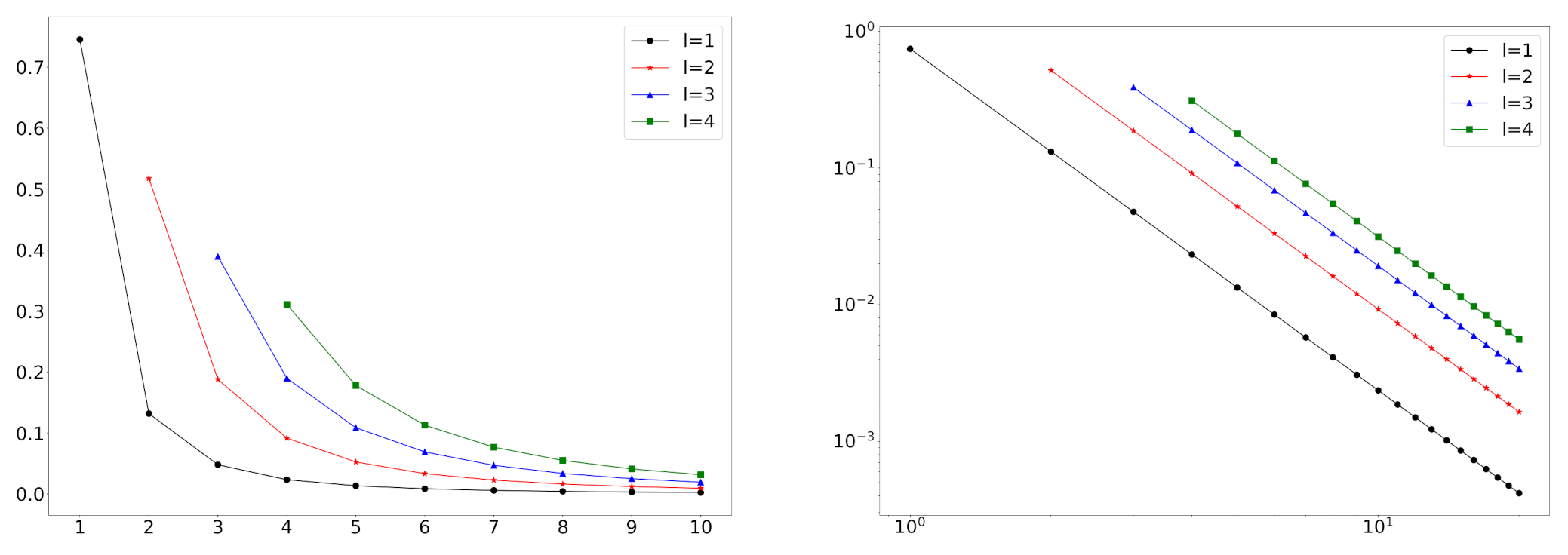
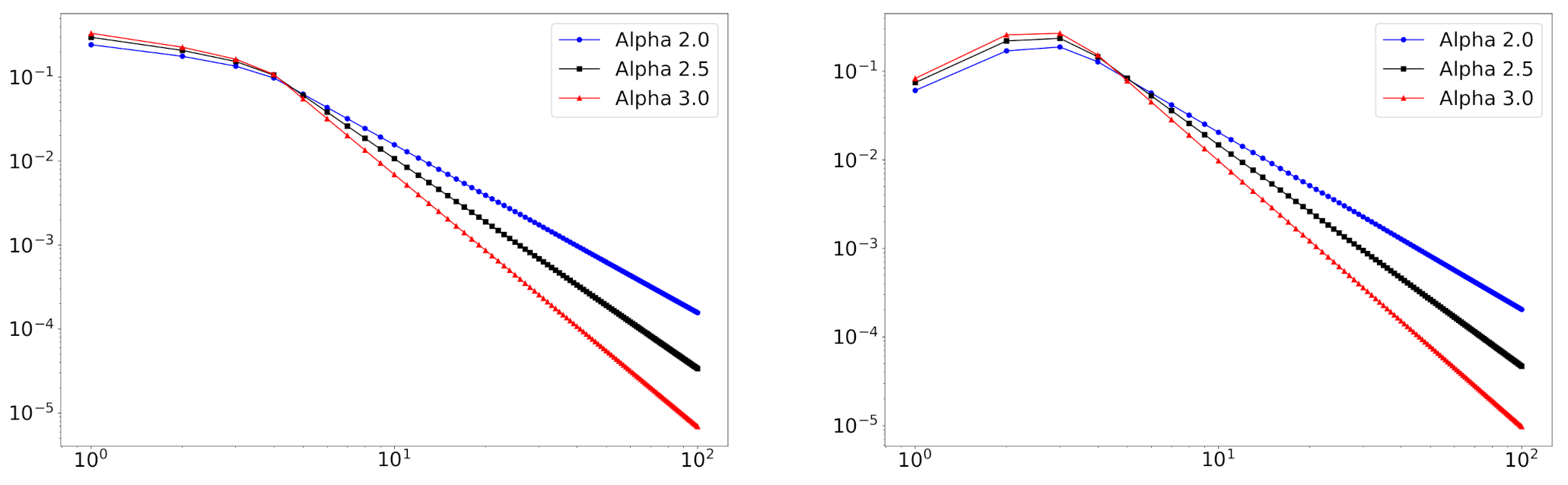
In
Figure 2, we depict some log-log plots of mixture distributions. We can see that this model can handle empirical degree distributions that do not follow the power-law distribution at small degrees.
4. Estimation Algorithm
We use the Expectation-Maximization (EM) algorithm to estimate the exponent parameter and mixture weights w for a given number of mixture components L. Let be the observed data, and be the membership of , where the membership is assigned as if is from the lth mixture component . We consider the membership variable as missing. Let be the parameters of the mixture model.
The complete-data likelihood function is given by
We proceed by taking the logarithms of both sides to have the complete-data log-likelihood function:
We define
as the expected value of the log-likelihood given the observed data
k and the current parameter estimate
, which can be expressed as
where
is the
membership responsibility of the
nth observation
corresponding to the
lth mixture component
. They are defined by the posterior probabilities of mixture component memberships for each observation,
The E-step computes membership responsibilities.
In the M-step, a new parameter estimate
is computed using the quantity previously computed in the E-step. To find
, we need to solve the following optimization problem:
The Lagrange multiplier method yields
Next,
can be found in the partial derivative of
Q with respect to
, given by
Here,
is the partial derivative of the Hurwitz zeta function with respect to
, given by
Then, the equation
gives the desired
. Unfortunately, a closed-form solution does not exist in general. In this paper, we employ Brent’s method [
34] to solve Equation (
10) with respect to
.
The two steps are necessarily repeated until the convergence obtains the final parameter estimate . The process is summarized in Algorithm 1.
In order to select the number of mixture components
L, we employ the Bayesian information criterion (BIC) considering the trade-off between the goodness-of-fit and the complexity of the model. BIC is given by the following formula:
where
and
w are the obtained estimated parameters given the number of mixture components
L. We choose
L giving the smallest BIC, where the candidates of
L are the integers from 1 to the minimum of the two values: 100 and the nearest integer to 0.90
.
| Algorithm 1: EM Algorithm |
 |
7. Concluding Remark
Inspired by Jordan’s model [
29], a novel mixture model for the degree distribution is proposed to describe the entire range of degrees while maintaining the power-law or the scale-free property of a network. The truncated zeta distribution enables us to analyze discrete distributions for accuracy purposes. The parameter estimation procedure is presented along with the model selection criterion for determining the number of mixture components. A simulation study shows the validity of the suggested estimation procedure. The practical performance of the model is studied through the comparison analysis with the other techniques.
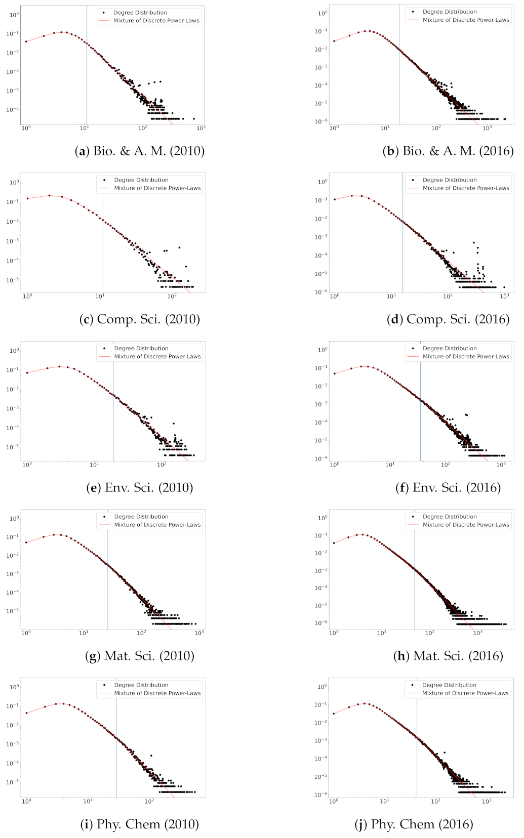
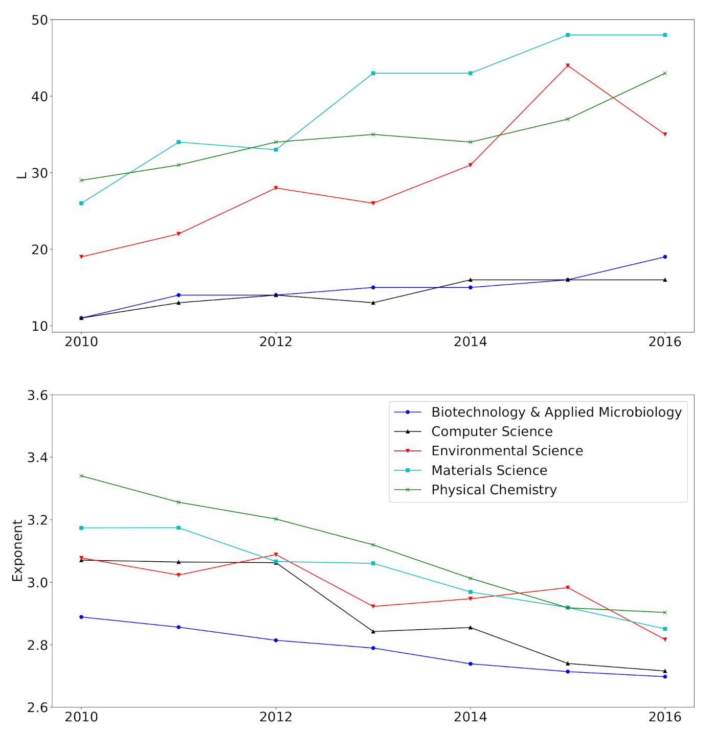
We perform the real data analysis on five disciplines of the scientific collaboration data obtained from the Web of Science. We observe the increasing tendency in the number of mixture components and the decreasing tendency in the power-law exponent. In addition, mixture weights change over time. It can be suggested from these results that the analyzed networks are still in an evolving state, highlighting the practical importance of non-stationary temporal network models. The non-convergence of the degree distribution might be due to the short-term analysis performed. Determining whether the collaboration network will stabilize the equilibrium remains as future work.
We can observe power-law distributions not only in the degree distribution but also in sandpile avalanches, species extinctions, city sizes, and so on. The proposed model could be useful when (i) the distribution does not follow the power-law only in small values while the power-law is suitable for large values, (ii) the background knowledge does not support the manual modification of the power-law relationship, or (iii) a mixture distribution can be regarded as reasonable for describing data.


