
Non Stationary Multi-Armed Bandit: Empirical Evaluation of a New Concept Drift-Aware Algorithm


Abstract
1. Introduction
2. Background
2.1. Multi-Armed Bandit
- ϵ-greedy. Given a small value , the agent selects a random arm with probability and the best arm a, where , with probability .
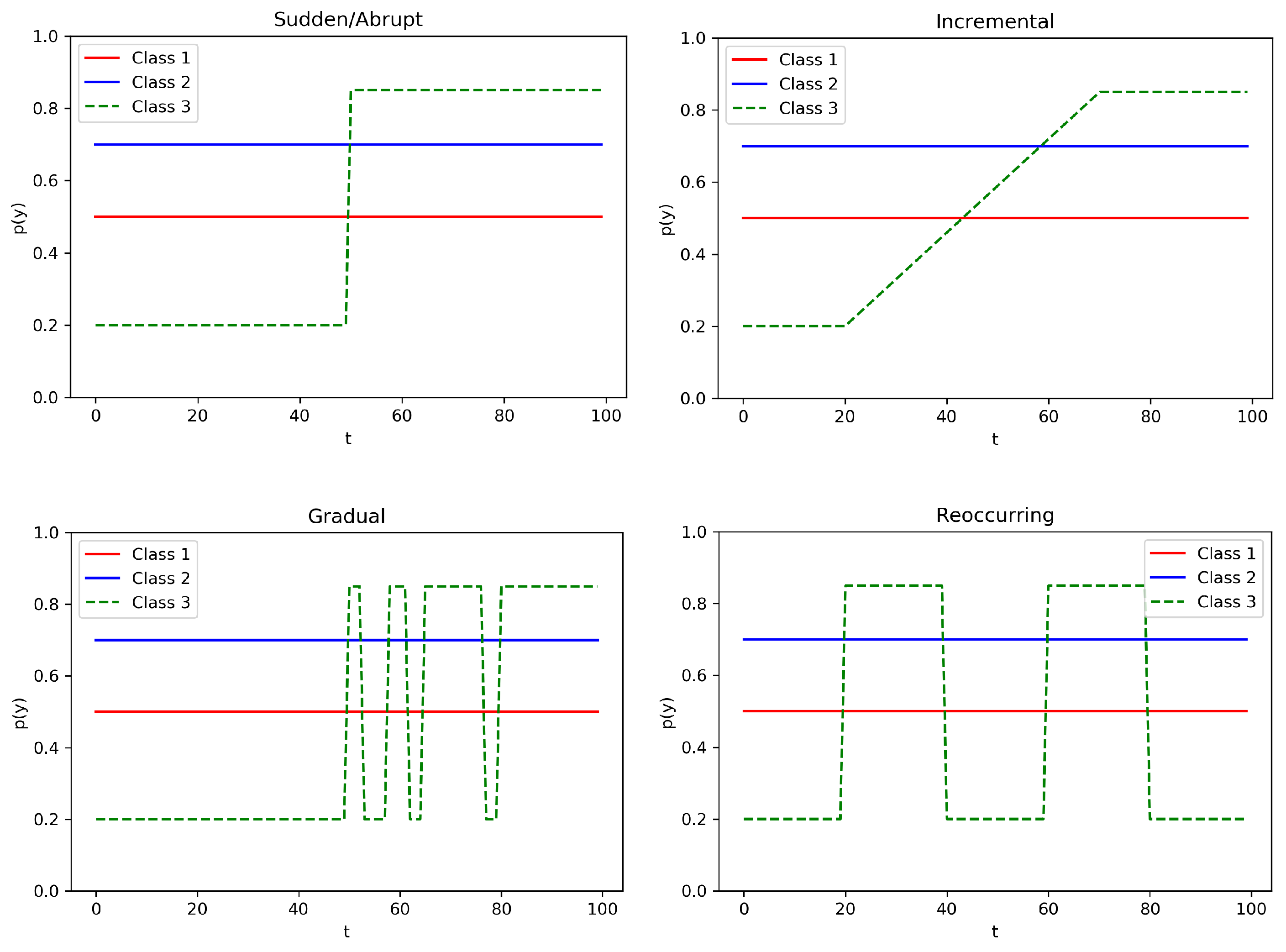
2.2. Concept Drift
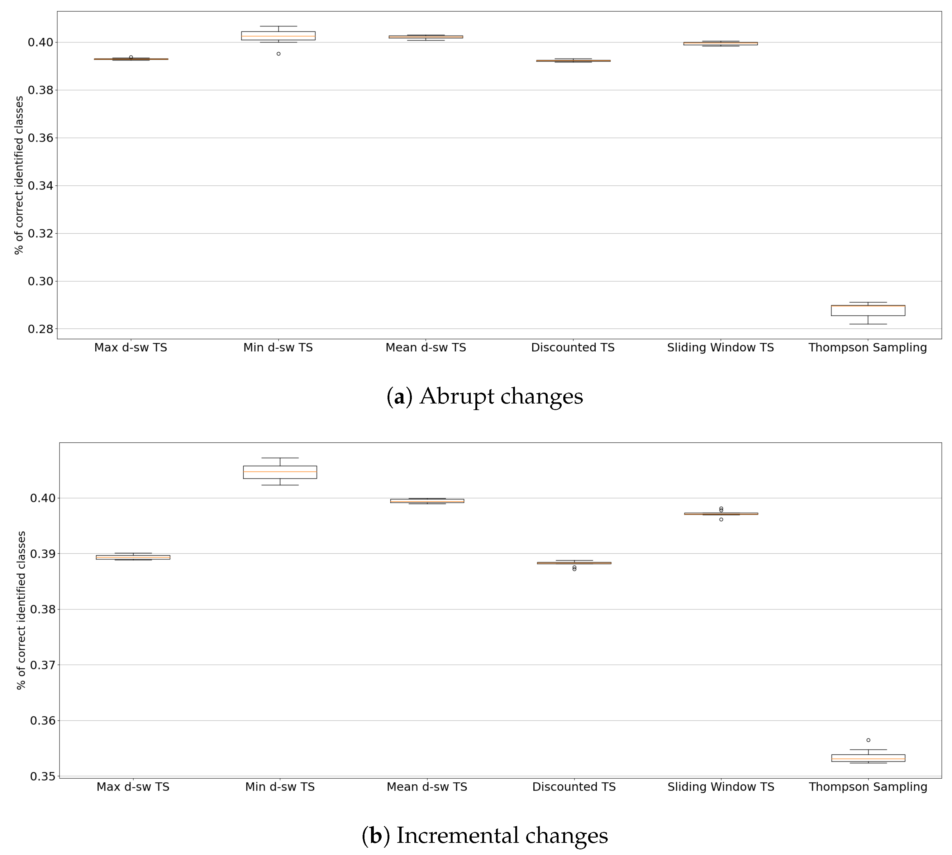
- Sudden/Abrupt: the switch of concept happens abruptly, from time to the subsequent time .
- Incremental: the switch of concept happens incrementally (slowly), with many smaller intermediate changes, from time to time .
- Gradual: the switch of concept happens gradually, by switching back and forth to the old and new concept, from time to time , before stabilizing to the new one.
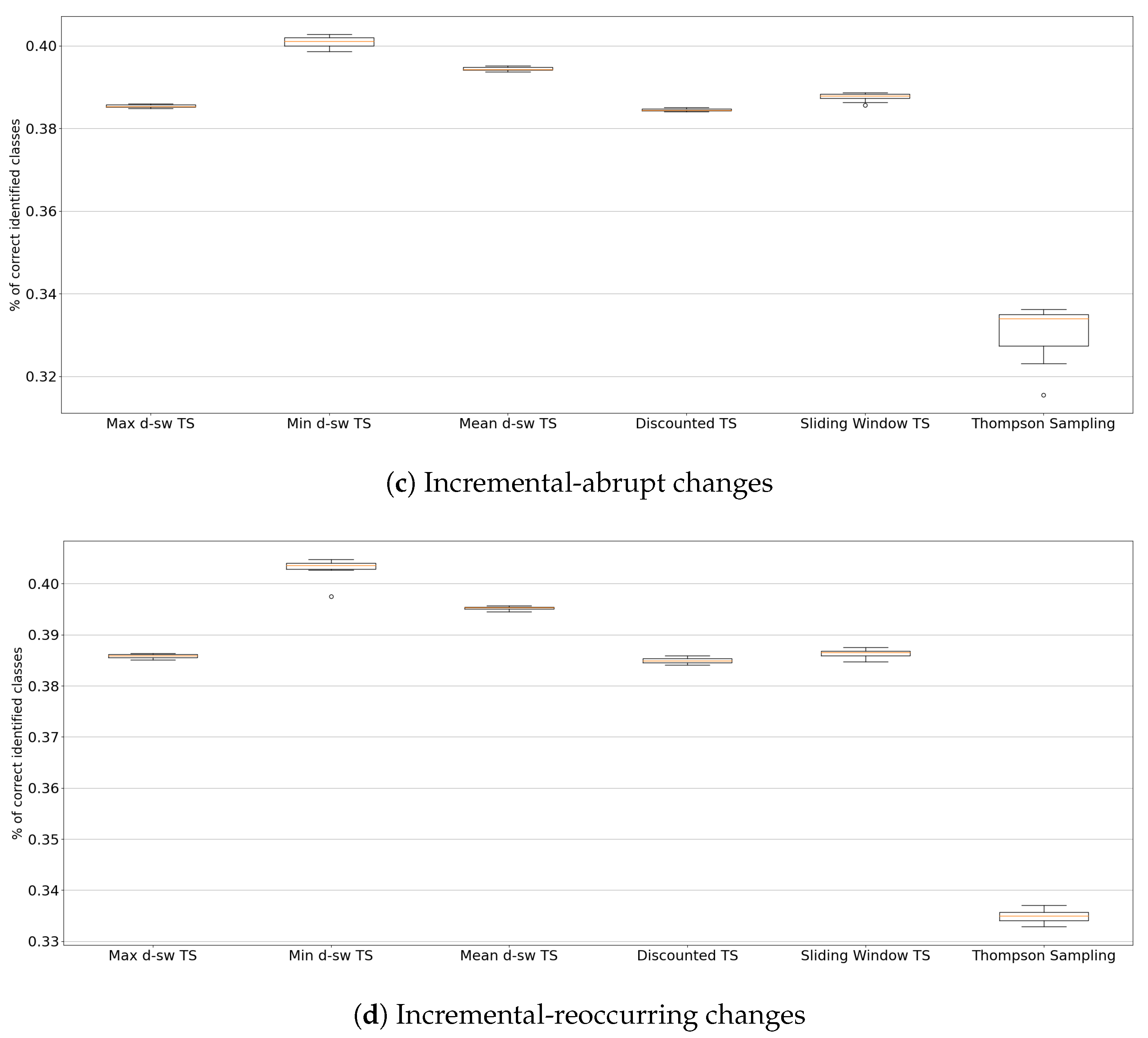
- Reocurring: The switch of concept happens abruptly at time , but after time the concept reverses back to the old one. It could be cyclic.
2.3. Non-Stationary Multi-Armed Bandit
3. Methodology
3.1. Problem Definition
3.2. f-Discounted-Sliding-Window Thompson Sampling
| Algorithm 1:f-Discounted-Sliding-Window TS |
 |
4. Experiments
4.1. Experimental Setup
- Max-dsw TS: f-dsw TS with max as an aggregation function f.
- Min-dsw TS: f-dsw TS with min as an aggregation function f.
- Mean-dsw TS: f-dsw TS with mean as an aggregation function f.
- Discounted TS: the TS enhanced with a discount factor, presented in [36]: the parameter controls the amount of discount.
- Sliding Window TS: the TS with a global sliding window, presented in [15]. The parameter n controls the size of the sliding window.
- Thompson Sampling: the standard Beta-Bernoulli TS.
- Random: a trivial baseline that selects each arm at random.
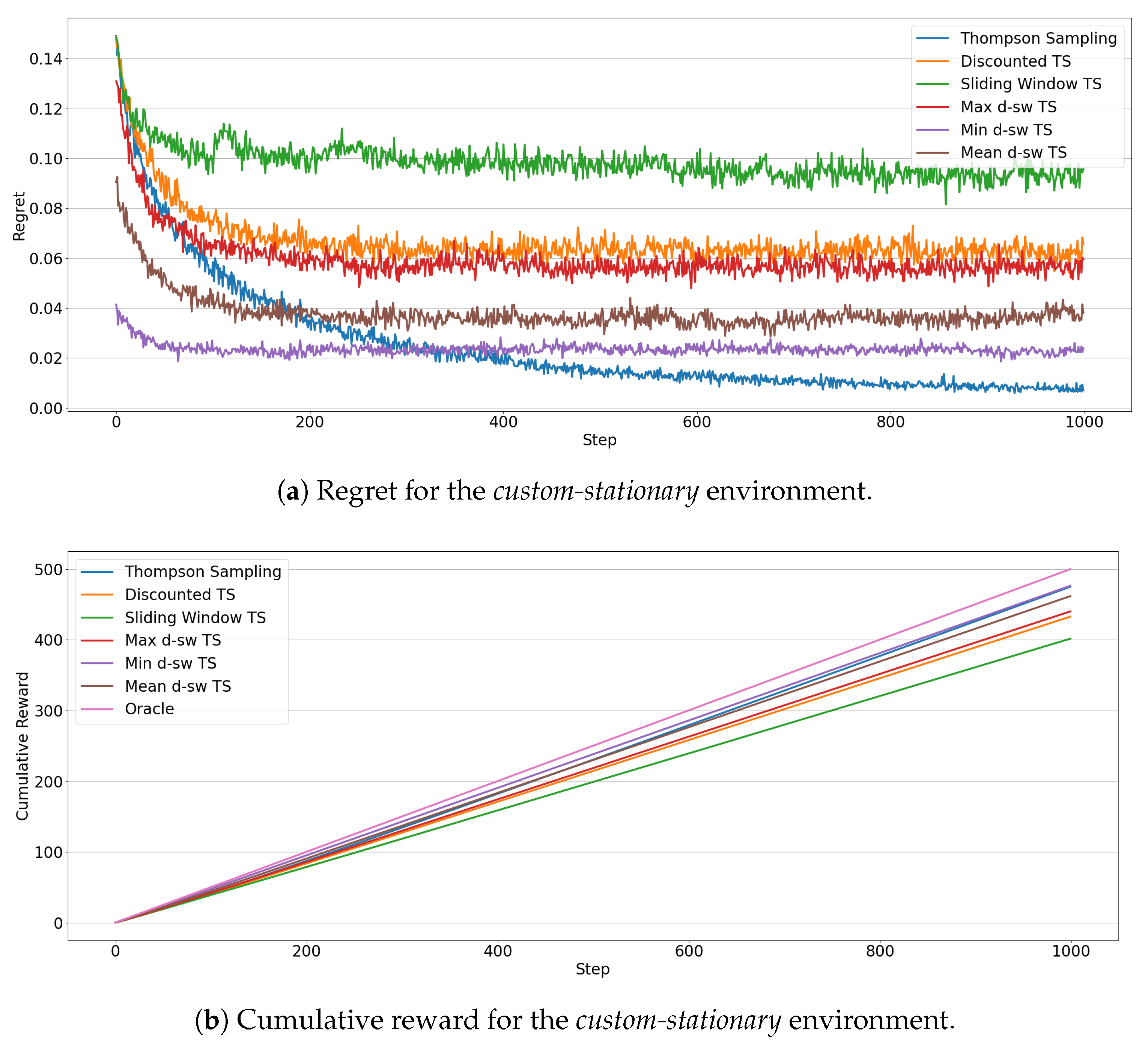
- Oracle: an oracle always selecting the best action at time t. It is exploited for regret computation.
4.2. Synthetic Datasets
4.2.1. Random Environments
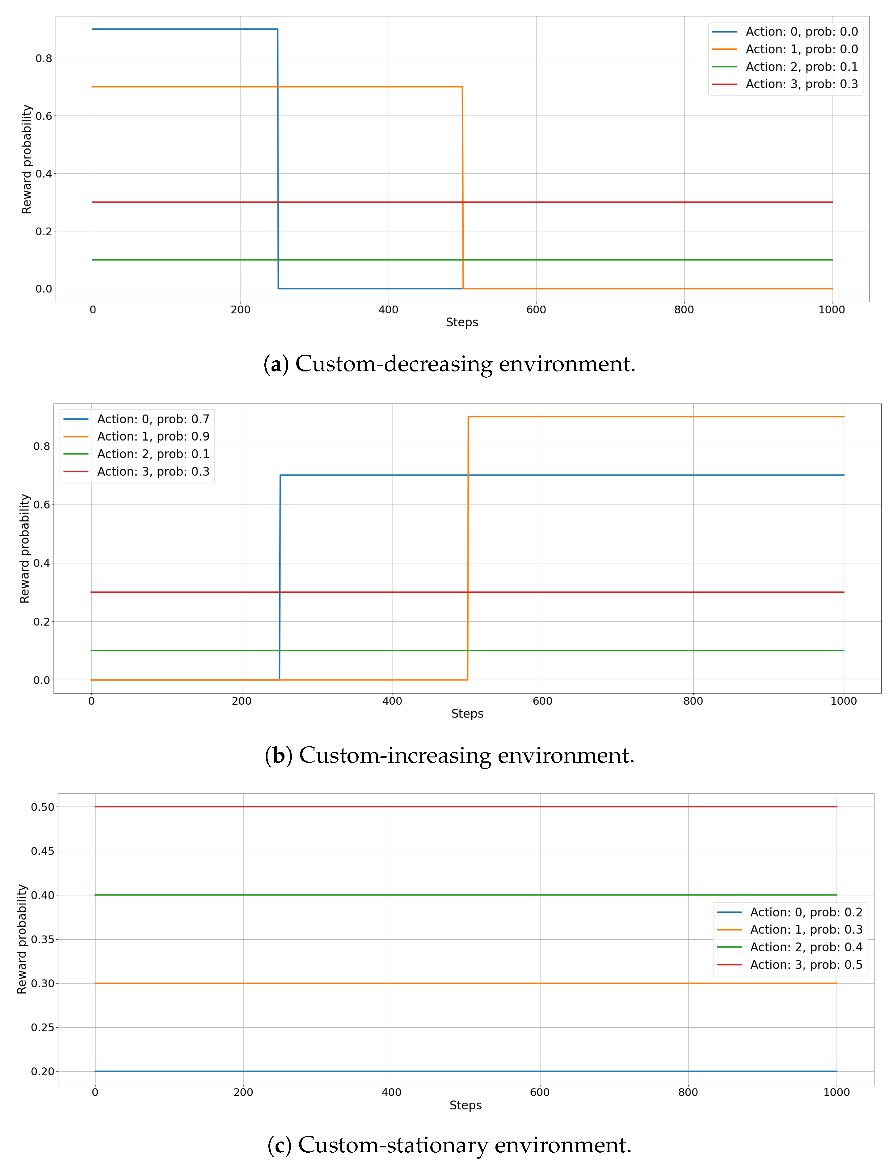
4.2.2. Custom Environments
4.3. Real Datasets
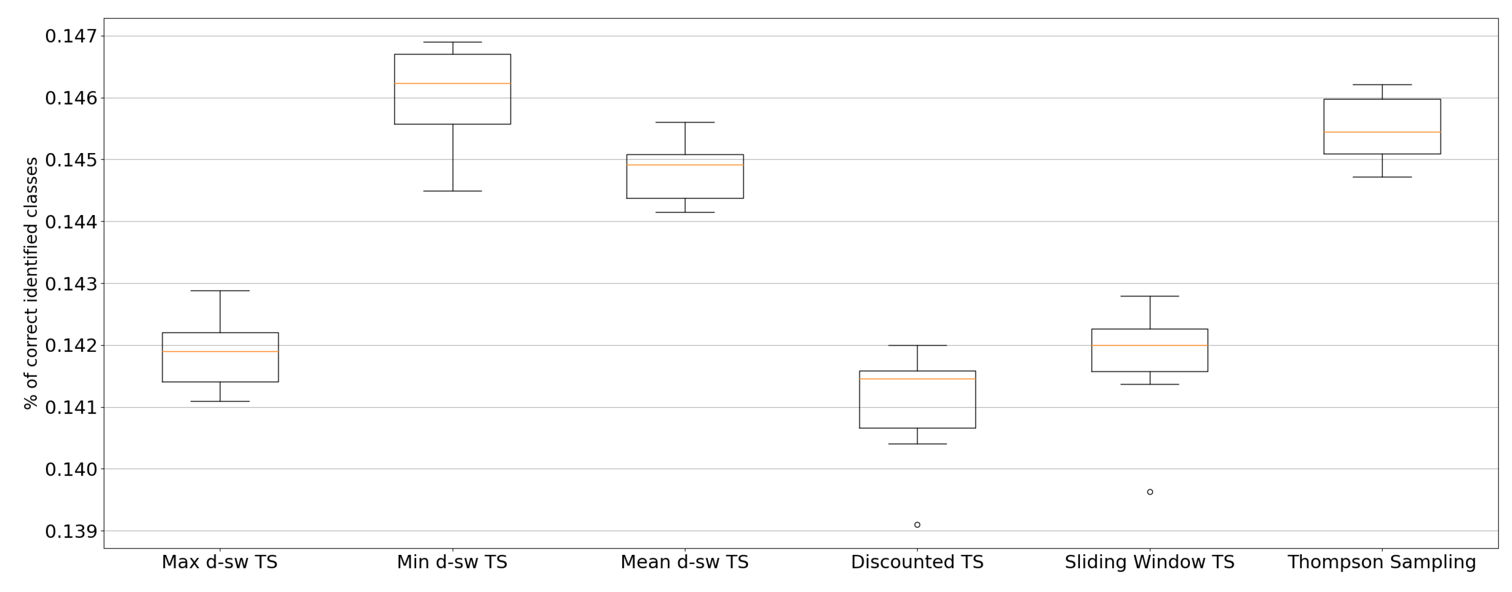
4.3.1. Baltimore Crime
4.3.2. Insects
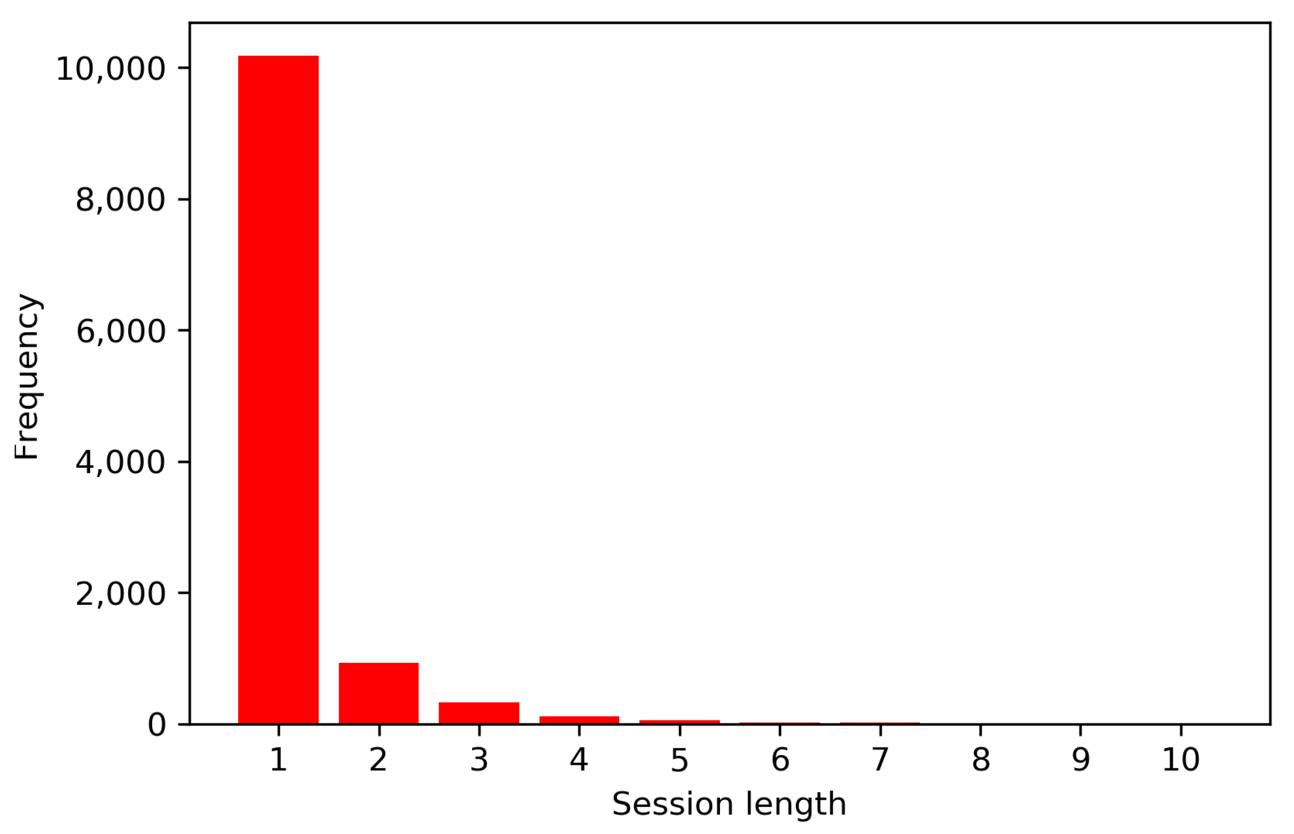
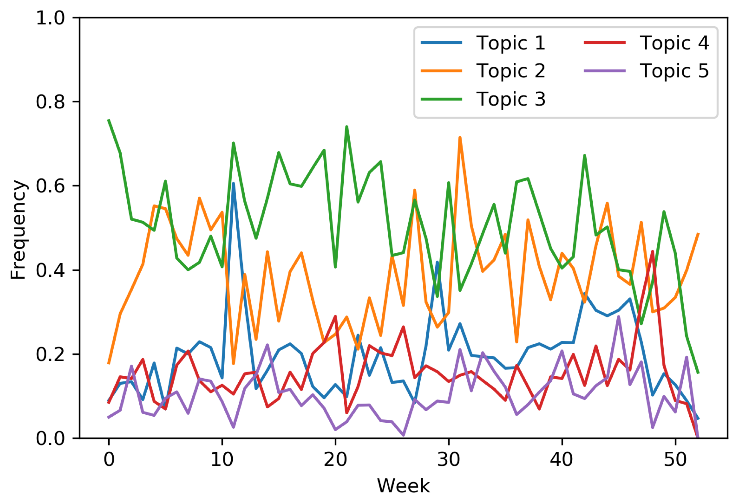
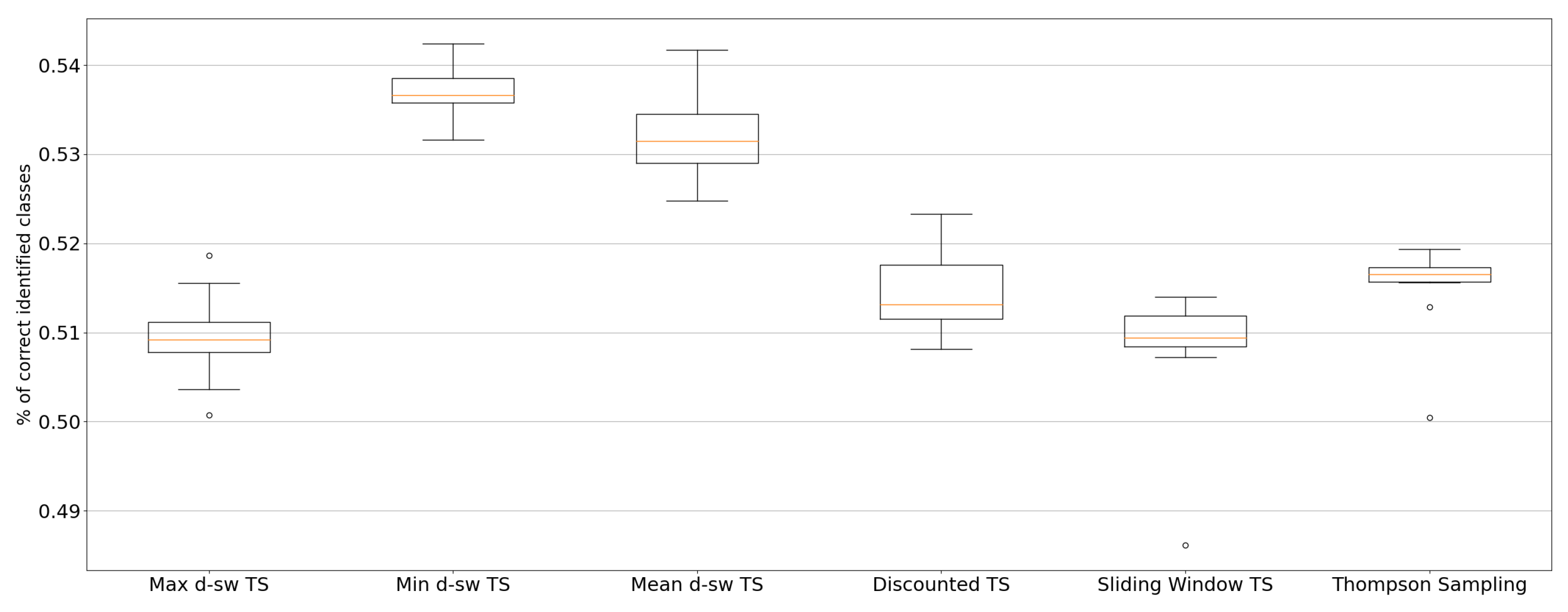
4.3.3. Local News
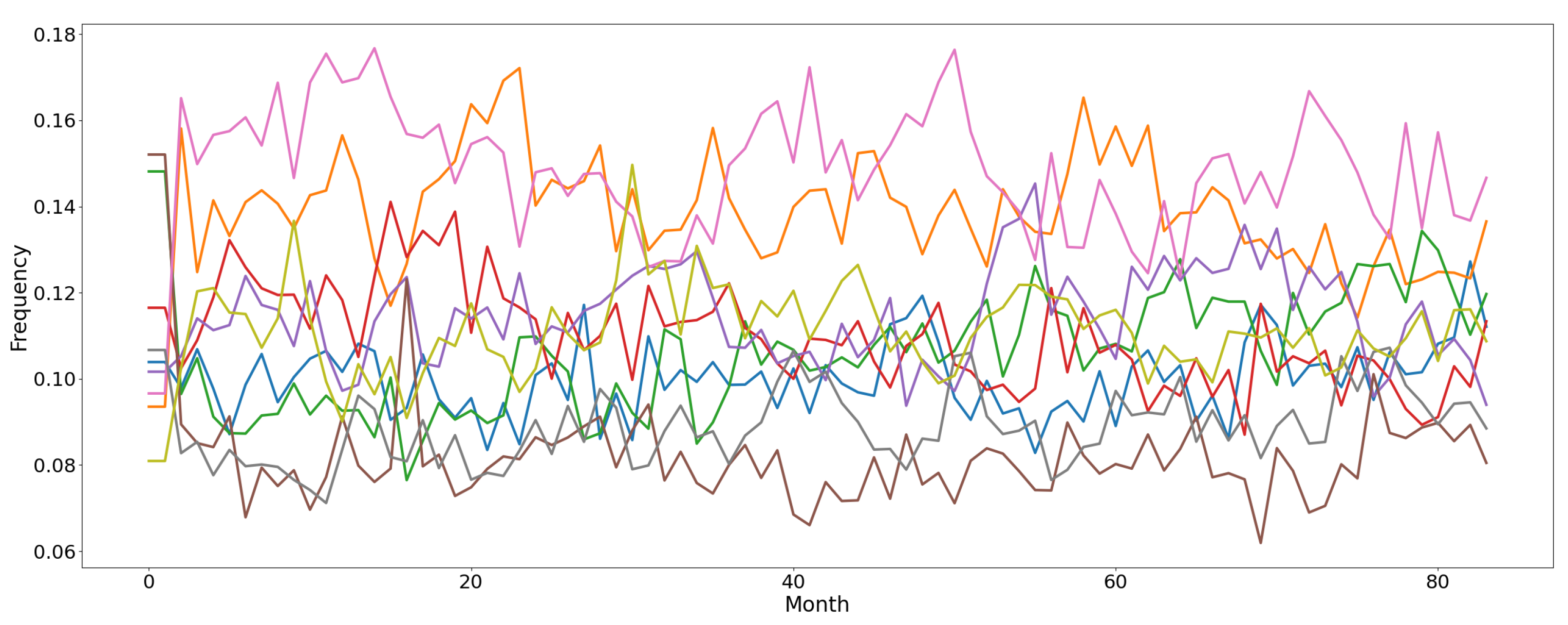
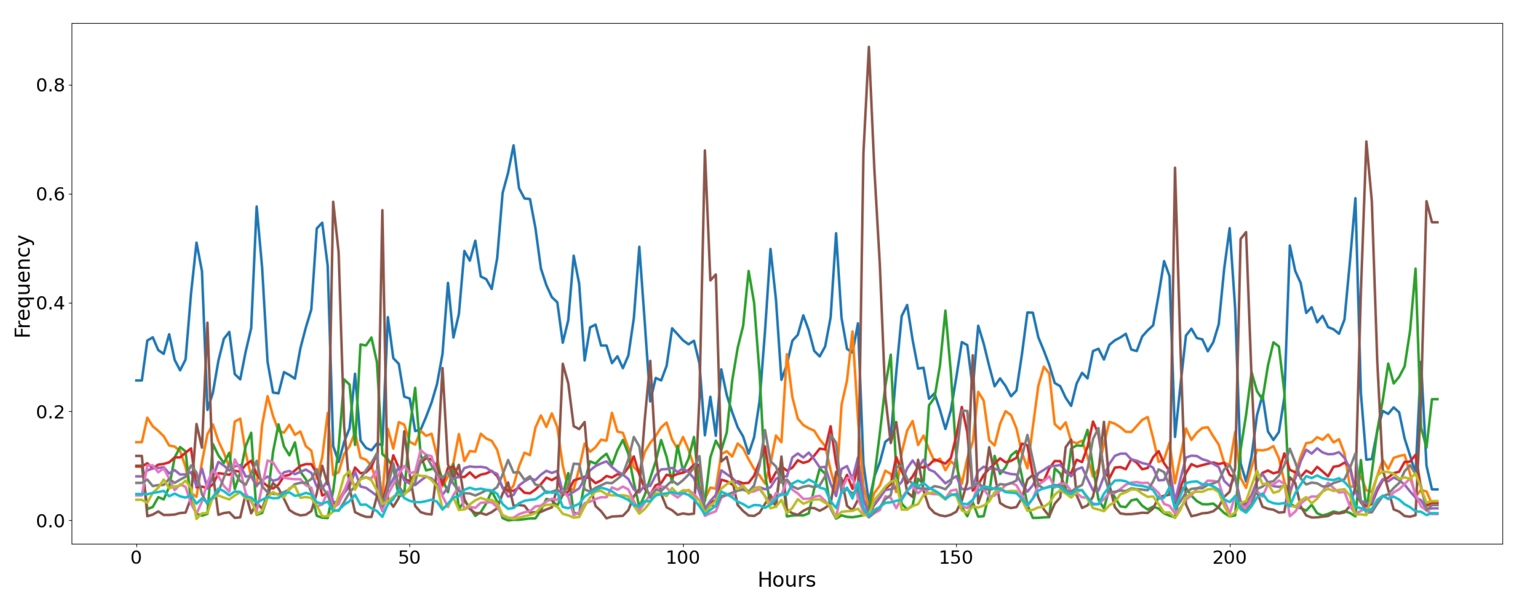
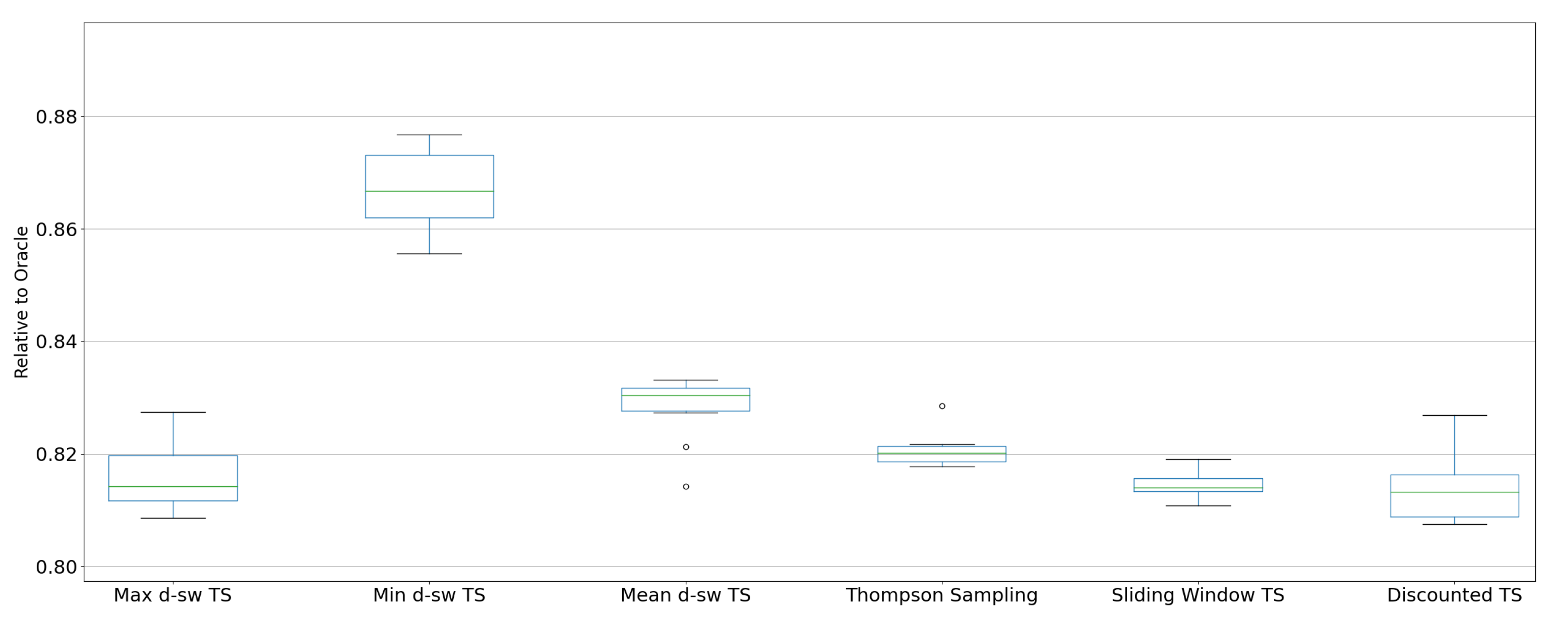
4.3.4. Air Microbes
4.4. Parameters Tuning
5. Results
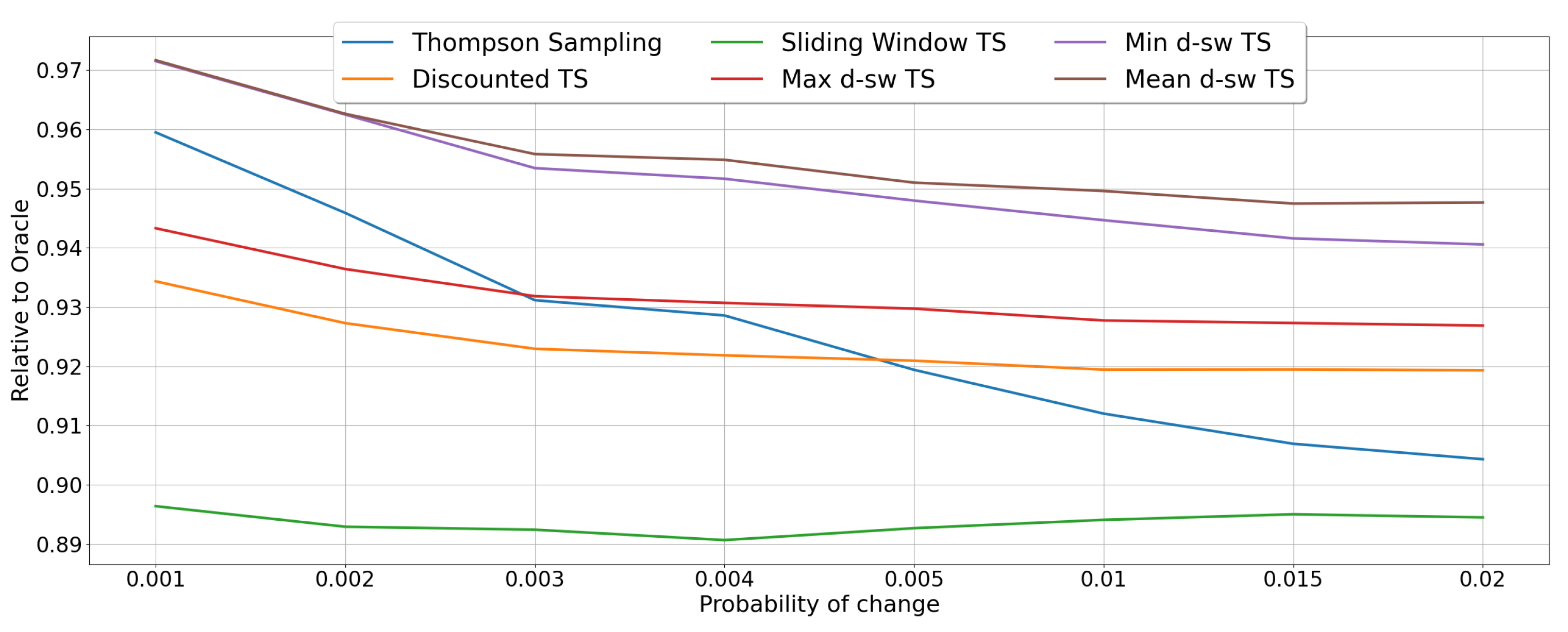
5.1. Random Environments
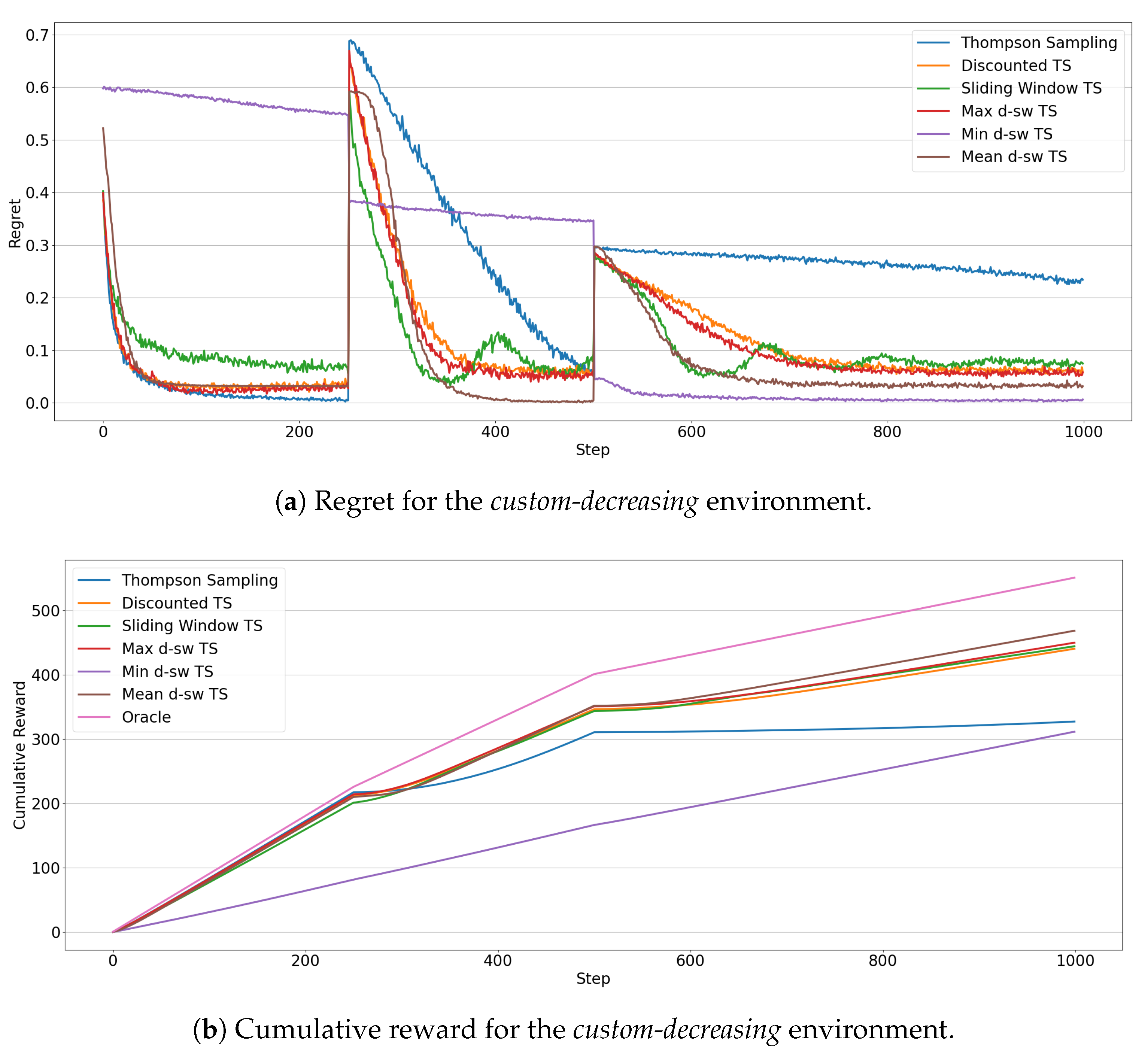
5.2. Custom Environments
5.3. Real-World Environments
6. Conclusions
Author Contributions
Funding
Institutional Review Board Statement
Informed Consent Statement
Data Availability Statement
Acknowledgments
Conflicts of Interest
Appendix A


References
- Robbins, H. Some aspects of the sequential design of experiments. Bull. Am. Math. Soc. 1952, 58, 527–535. [Google Scholar] [CrossRef]
- Berry, D.A.; Fristedt, B. Bandit Problems: Sequential Allocation of Experiments (Monographs on Statistics and Applied Probability); Chapman Hall: London, UK, 1985; Volume 5, p. 7. [Google Scholar]
- Kuleshov, V.; Precup, D. Algorithms for multi-armed bandit problems. arXiv 2014, arXiv:1402.6028. [Google Scholar]
- Villar, S.S.; Bowden, J.; Wason, J. Multi-armed bandit models for the optimal design of clinical trials: Benefits and challenges. Stat. Sci. A Rev. J. Inst. Math. Stat. 2015, 30, 199. [Google Scholar] [CrossRef]
- Ding, W.; Qin, T.; Zhang, X.D.; Liu, T.Y. Multi-Armed Bandit with Budget Constraint and Variable Costs. In Proceedings of the AAAI Conference on Artificial Intelligence, Bellevue, WA, USA, 14–18 July 2013; Volume 13, pp. 232–238. [Google Scholar]
- Schwartz, E.M.; Bradlow, E.T.; Fader, P.S. Customer acquisition via display advertising using multi-armed bandit experiments. Mark. Sci. 2017, 36, 500–522. [Google Scholar] [CrossRef]
- Le Ny, J.; Dahleh, M.; Feron, E. Multi-UAV dynamic routing with partial observations using restless bandit allocation indices. In Proceedings of the 2008 American Control Conference, Seattle, WA, USA, 11–13 June 2008; pp. 4220–4225. [Google Scholar]
- Scott, S.L. A Modern Bayesian Look at the Multi-Armed Bandit. Appl. Stoch. Model. Bus. Ind. 2010, 26, 639–658. [Google Scholar] [CrossRef]
- Chapelle, O.; Li, L. An Empirical Evaluation of Thompson Sampling. In Proceedings of the 24th International Conference on Neural Information Processing Systems (NIPS’11), Granada, Spain, 12–14 December 2011; Curran Associates Inc.: Red Hook, NY, USA, 2011; pp. 2249–2257. [Google Scholar]
- Li, L.; Chu, W.; Langford, J.; Schapire, R.E. A Contextual-Bandit Approach to Personalized News Article Recommendation. In Proceedings of the 19th International Conference on World Wide Web (WWW’10), Raleigh, NC, USA, 26–30 April 2010; Association for Computing Machinery: New York, NY, USA, 2010; pp. 661–670. [Google Scholar] [CrossRef]
- Benedetto, G.D.; Bellini, V.; Zappella, G. A Linear Bandit for Seasonal Environments. arXiv 2020, arXiv:2004.13576. [Google Scholar]
- Besbes, O.; Gur, Y.; Zeevi, A. Stochastic multi-armed-bandit problem with non-stationary rewards. In Proceedings of the Advances in Neural Information Processing Systems, Montreal, QC, Canada, 8–13 December 2014; pp. 199–207. [Google Scholar]
- Gama, J.; Žliobaitė, I.; Bifet, A.; Pechenizkiy, M.; Bouchachia, A. A survey on concept drift adaptation. ACM Comput. Surv. CSUR 2014, 46, 1–37. [Google Scholar] [CrossRef]
- Zliobaite, I. Learning under Concept Drift: An Overview. arXiv 2010, arXiv:1010.4784. [Google Scholar]
- Trovo, F.; Paladino, S.; Restelli, M.; Gatti, N. Sliding-Window Thompson Sampling for Non-Stationary Settings. J. Artif. Intell. Res. 2020, 68, 311–364. [Google Scholar] [CrossRef]
- Slivkins, A. Introduction to Multi-Armed Bandits. arXiv 2019, arXiv:1904.07272. [Google Scholar]
- Agrawal, R. Sample mean based index policies with O (log n) regret for the multi-armed bandit problem. Adv. Appl. Probab. 1995, 27, 1054–1078. [Google Scholar] [CrossRef]
- Auer, P. Using confidence bounds for exploitation-exploration trade-offs. J. Mach. Learn. Res. 2002, 3, 397–422. [Google Scholar]
- Thompson, W.R. On the likelihood that one unknown probability exceeds another in view of the evidence of two samples. Biometrika 1933, 25, 285–294. [Google Scholar] [CrossRef]
- Thompson, W.R. On the theory of apportionment. Am. J. Math. 1935, 57, 450–456. [Google Scholar] [CrossRef]
- Russo, D.; Roy, B.V.; Kazerouni, A.; Osband, I.; Wen, Z. A Tutorial on Thompson Sampling. arXiv 2017, arXiv:1707.02038. [Google Scholar]
- Auer, P.; Cesa-Bianchi, N.; Fischer, P. Finite-time analysis of the multiarmed bandit problem. Mach. Learn. 2002, 47, 235–256. [Google Scholar] [CrossRef]
- Kaufmann, E.; Korda, N.; Munos, R. Thompson sampling: An asymptotically optimal finite-time analysis. In Proceedings of the International Conference on Algorithmic Learning Theory, Lyon, France, 29–31 October 2012; Springer: Berlin/Heidelberger, Germany, 2012; pp. 199–213. [Google Scholar]
- Agrawal, S.; Goyal, N. Analysis of thompson sampling for the multi-armed bandit problem. In Proceedings of the Conference on Learning Theory, Edinburgh, UK, 25–27 June 2012. [Google Scholar]
- Russo, D.; Van Roy, B. An Information-Theoretic Analysis of Thompson Sampling. J. Mach. Learn. Res. 2016, 17, 2442–2471. [Google Scholar]
- Russo, D.; Van Roy, B. Learning to Optimize via Information-Directed Sampling. Oper. Res. 2018, 66, 230–252. [Google Scholar] [CrossRef]
- Chow, S.C.; Chang, M. Adaptive Design Methods in Clinical Trials, 2nd ed.; CRC Press: New York, NY, USA, 2006; Volume 3. [Google Scholar] [CrossRef]
- Srinivas, N.; Krause, A.; Kakade, S.; Seeger, M. Gaussian Process Optimization in the Bandit Setting: No Regret and Experimental Design; Omnipress: Madison, WI, USA, 2010; pp. 1015–1022. [Google Scholar]
- Brochu, E.; Brochu, T.; de Freitas, N. A Bayesian Interactive Optimization Approach to Procedural Animation Design. In Proceedings of the 2010 ACM SIGGRAPH/Eurographics Symposium on Computer Animation (SCA’10), Madrid, Spain, 2–4 July 2010; Eurographics Association: Goslar, Germany, 2010; pp. 103–112. [Google Scholar]
- Lu, J.; Liu, A.; Dong, F.; Gu, F.; Gama, J.; Zhang, G. Learning under concept drift: A review. IEEE Trans. Knowl. Data Eng. 2018, 31, 2346–2363. [Google Scholar] [CrossRef]
- Žliobaitė, I.; Pechenizkiy, M.; Gama, J. An overview of concept drift applications. In Big Data Analysis: New Algorithms for a New Society; Springer: Berlin, Germany, 2016; pp. 91–114. [Google Scholar]
- Dries, A.; Rückert, U. Adaptive Concept Drift Detection. Stat. Anal. Data Min. 2009, 2, 311–327. [Google Scholar] [CrossRef]
- Klinkenberg, R.; Joachims, T. Detecting Concept Drift with Support Vector Machines. In Proceedings of the Seventeenth International Conference on Machine Learning (ICML’00), Standord, CA, USA, 29 June–2 July 2000; Morgan Kaufmann Publishers Inc.: San Francisco, CA, USA, 2000; pp. 487–494. [Google Scholar]
- Nishida, K.; Yamauchi, K. Detecting Concept Drift Using Statistical Testing. In Discovery Science; Corruble, V., Takeda, M., Suzuki, E., Eds.; Springer: Berlin/Heidelberg, Germany, 2007; pp. 264–269. [Google Scholar]
- Elwell, R.; Polikar, R. Incremental Learning of Concept Drift in Nonstationary Environments. IEEE Trans. Neural Netw. 2011, 22, 1517–1531. [Google Scholar] [CrossRef] [PubMed]
- Raj, V.; Kalyani, S. Taming non-stationary bandits: A Bayesian approach. arXiv 2017, arXiv:1707.09727. [Google Scholar]
- Garivier, A.; Moulines, E. On upper-confidence bound policies for non-stationary bandit problems. arXiv 2008, arXiv:0805.3415. [Google Scholar]
- Fouché, E.; Komiyama, J.; Böhm, K. Scaling multi-armed bandit algorithms. In Proceedings of the 25th ACM SIGKDD International Conference on Knowledge Discovery & Data Mining, Anchorage, AK, USA, 4–8 August 2019; pp. 1449–1459. [Google Scholar]
- Bifet, A.; Gavalda, R. Learning from time-changing data with adaptive windowing. In Proceedings of the 2007 SIAM International Conference on Data Mining, Minneapolis, MN, USA, 26–28 April 2007; pp. 443–448. [Google Scholar]
- Hartland, C.; Gelly, S.; Baskiotis, N.; Teytaud, O.; Sebag, M. Multi-armed bandit, dynamic environments and meta-bandits. In Proceedings of the NIPS-2006 Workshop, Online Trading between Exploration and Exploitation, Whistler, BC, Canada, 8 December 2006. [Google Scholar]
- Kaufmann, E.; Cappé, O.; Garivier, A. On Bayesian upper confidence bounds for bandit problems. In Proceedings of the Artificial Intelligence and Statistics, Canary Islands, Spain, 21–23 April 2012; pp. 592–600. [Google Scholar]
- May, B.C.; Korda, N.; Lee, A.; Leslie, D.S. Optimistic Bayesian sampling in contextual-bandit problems. J. Mach. Learn. Res. 2012, 13, 2069–2106. [Google Scholar]
- Mellor, J.; Shapiro, J. Thompson sampling in switching environments with Bayesian online change detection. In Proceedings of the Artificial Intelligence and Statistics, Scottsdale, AZ, USA, 29 April–1 May 2013; pp. 442–450. [Google Scholar]
- Liu, F.; Lee, J.; Shroff, N. A change-detection based framework for piecewise-stationary multi-armed bandit problem. arXiv 2017, arXiv:1711.03539. [Google Scholar]
- Besson, L.; Kaufmann, E. The generalized likelihood ratio test meets klucb: An improved algorithm for piece-wise non-stationary bandits. arXiv 2019, arXiv:1902.01575. [Google Scholar]
- KhudaBukhsh, A.R.; Carbonell, J.G. Expertise drift in referral networks. Auton. Agents Multi-Agent Syst. 2019, 33, 645–671. [Google Scholar] [CrossRef]
- St-Pierre, D.L.; Liu, J. Differential evolution algorithm applied to non-stationary bandit problem. In Proceedings of the 2014 IEEE Congress on Evolutionary Computation (CEC), Beijing, China, 6–11 July 2014; pp. 2397–2403. [Google Scholar]
- Allesiardo, R.; Féraud, R.; Maillard, O.A. The non-stationary stochastic multi-armed bandit problem. Int. J. Data Sci. Anal. 2017, 3, 267–283. [Google Scholar] [CrossRef]
- Souza, V.; Reis, D.M.d.; Maletzke, A.G.; Batista, G.E. Challenges in Benchmarking Stream Learning Algorithms with Real-world Data. arXiv 2020, arXiv:2005.00113. [Google Scholar]
- Sottocornola, G.; Symeonidis, P.; Zanker, M. Session-Based News Recommendations. In Proceedings of the Companion Proceedings of the The Web Conference 2018 (WWW’18), Lyon, France, 23–27 April 2018; International World Wide Web Conferences Steering Committee: Geneva, Switzerland, 2018; pp. 1395–1399. [Google Scholar] [CrossRef]
- Blei, D.M. Probabilistic Topic Models. Commun. ACM 2012, 55, 77–84. [Google Scholar] [CrossRef]
- Gusareva, E.S.; Acerbi, E.; Lau, K.J.; Luhung, I.; Premkrishnan, B.N.; Kolundžija, S.; Purbojati, R.W.; Wong, A.; Houghton, J.N.; Miller, D.; et al. Microbial communities in the tropical air ecosystem follow a precise diel cycle. Proc. Natl. Acad. Sci. USA 2019, 116, 23299–23308. [Google Scholar] [CrossRef] [PubMed]


| Dataset | Classes | Instances | Time Span |
|---|---|---|---|
| Baltimore Crime | 9 | 321,147 | 6 years |
| Insects-Incremental | 6 | 452,045 | 3 months |
| Insects-Abrupt | 6 | 355,276 | 3 months |
| Insects-Incremental-gradual | 6 | 143,224 | 3 months |
| Insects-Incremental-abrupt-reoccurring | 6 | 452,045 | 3 months |
| Insects-Incremental-reoccurring | 6 | 452,045 | 3 months |
| Local News | 5 | 13,526 | 1 year |
| Air Microbes | 10 | 28,560 | 20 days |
| Algorithm | Random-Abrupt | Random-Incremental |
|---|---|---|
| Max-dsw TS | ||
| Min-dsw TS | ||
| Mean-dsw TS | ||
| Discounted TS | ||
| Sliding Window TS |
| Algorithm | Baltimore Crime | Insects | Local News | Air Microbes |
|---|---|---|---|---|
| Max-dsw TS | ||||
| Min-dsw TS | ||||
| Mean-dsw TS | ||||
| D-TS | ||||
| SW-TS |
| Dataset | Max-dsw | Min-dsw | Mean-dsw | D-TS | SW-TS | TS | Rand |
|---|---|---|---|---|---|---|---|
| Baltimore Crime | 14.18 | 14.61 | 14.48 | 14.11 | 14.18 | 14.55 | 10.85 |
| Insects abrupt | 39.30 | 40.24 | 40.21 | 39.22 | 39.94 | 28.8 | 16.65 |
| Insects incremental | 38.94 | 40.47 | 39.94 | 38.82 | 39.72 | 35.35 | 16.63 |
| Insects incr-abrupt-reoc | 38.54 | 40.10 | 39.44 | 38.45 | 38.77 | 33.05 | 16.69 |
| Insects incremental-reoc | 38.58 | 40.30 | 39.53 | 38.49 | 38.63 | 33.48 | 16.68 |
| Local News | 50.94 | 53.70 | 53.17 | 51.46 | 50.79 | 51.49 | 23.69 |
| Air Microbes * | 81.13 | 86.06 | 82.57 | 80.93 | 81.42 | 81.94 | 26.95 |
Publisher’s Note: MDPI stays neutral with regard to jurisdictional claims in published maps and institutional affiliations. |
© 2021 by the authors. Licensee MDPI, Basel, Switzerland. This article is an open access article distributed under the terms and conditions of the Creative Commons Attribution (CC BY) license (http://creativecommons.org/licenses/by/4.0/).
Share and Cite
Cavenaghi, E.; Sottocornola, G.; Stella, F.; Zanker, M. Non Stationary Multi-Armed Bandit: Empirical Evaluation of a New Concept Drift-Aware Algorithm. Entropy 2021, 23, 380. https://doi.org/10.3390/e23030380
Cavenaghi E, Sottocornola G, Stella F, Zanker M. Non Stationary Multi-Armed Bandit: Empirical Evaluation of a New Concept Drift-Aware Algorithm. Entropy. 2021; 23(3):380. https://doi.org/10.3390/e23030380
Chicago/Turabian StyleCavenaghi, Emanuele, Gabriele Sottocornola, Fabio Stella, and Markus Zanker. 2021. "Non Stationary Multi-Armed Bandit: Empirical Evaluation of a New Concept Drift-Aware Algorithm" Entropy 23, no. 3: 380. https://doi.org/10.3390/e23030380
APA StyleCavenaghi, E., Sottocornola, G., Stella, F., & Zanker, M. (2021). Non Stationary Multi-Armed Bandit: Empirical Evaluation of a New Concept Drift-Aware Algorithm. Entropy, 23(3), 380. https://doi.org/10.3390/e23030380