
Study of Wound Healing Dynamics by Single Pseudo-Particle Tracking in Phase Contrast Images Acquired in Time-Lapse

 , ,
, ,
Abstract
1. Introduction
2. Methods
2.1. Data
2.2. Image Processing
2.2.1. Equalization of the Frames
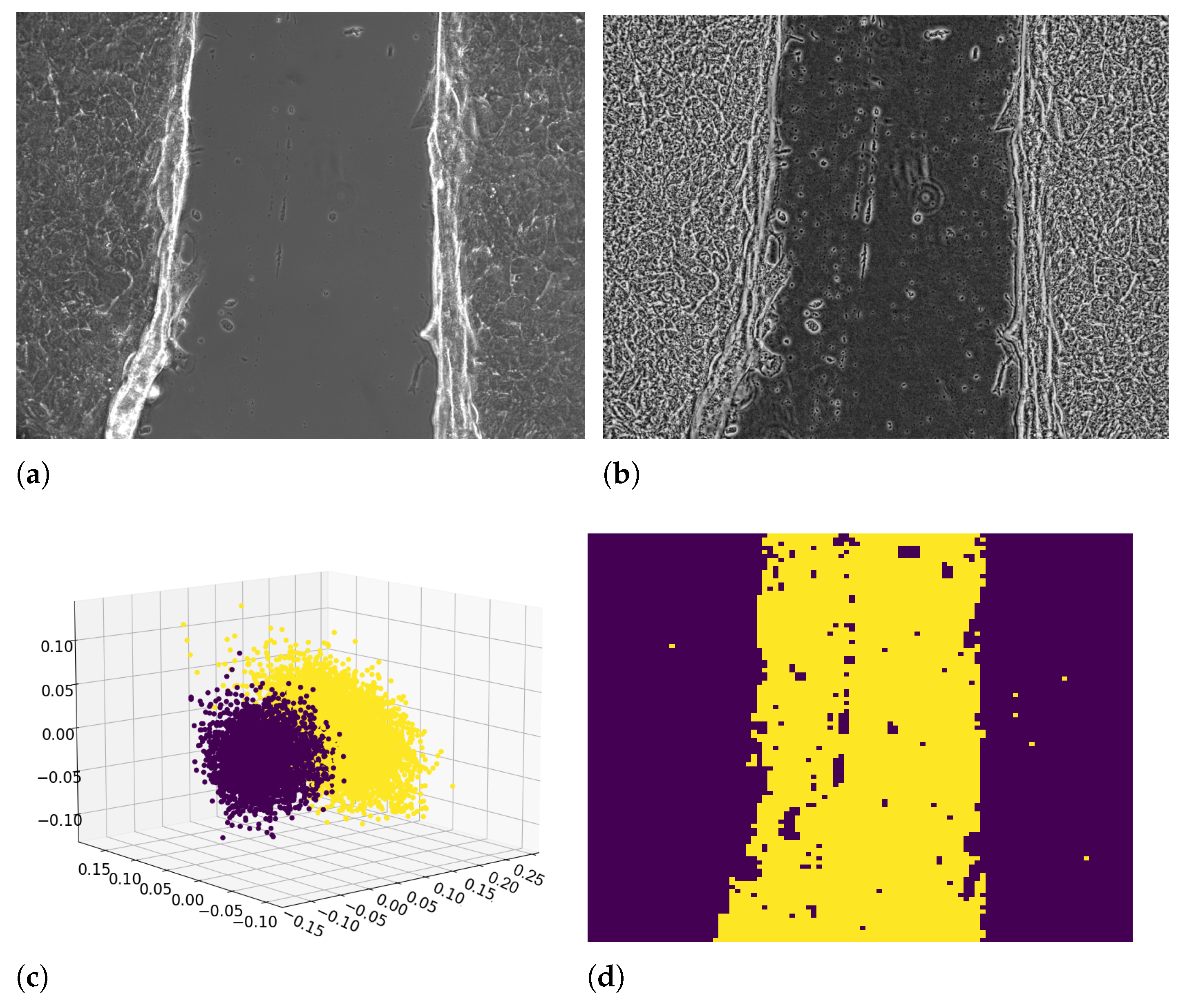
2.2.2. Image Binarization by Texture Analysis
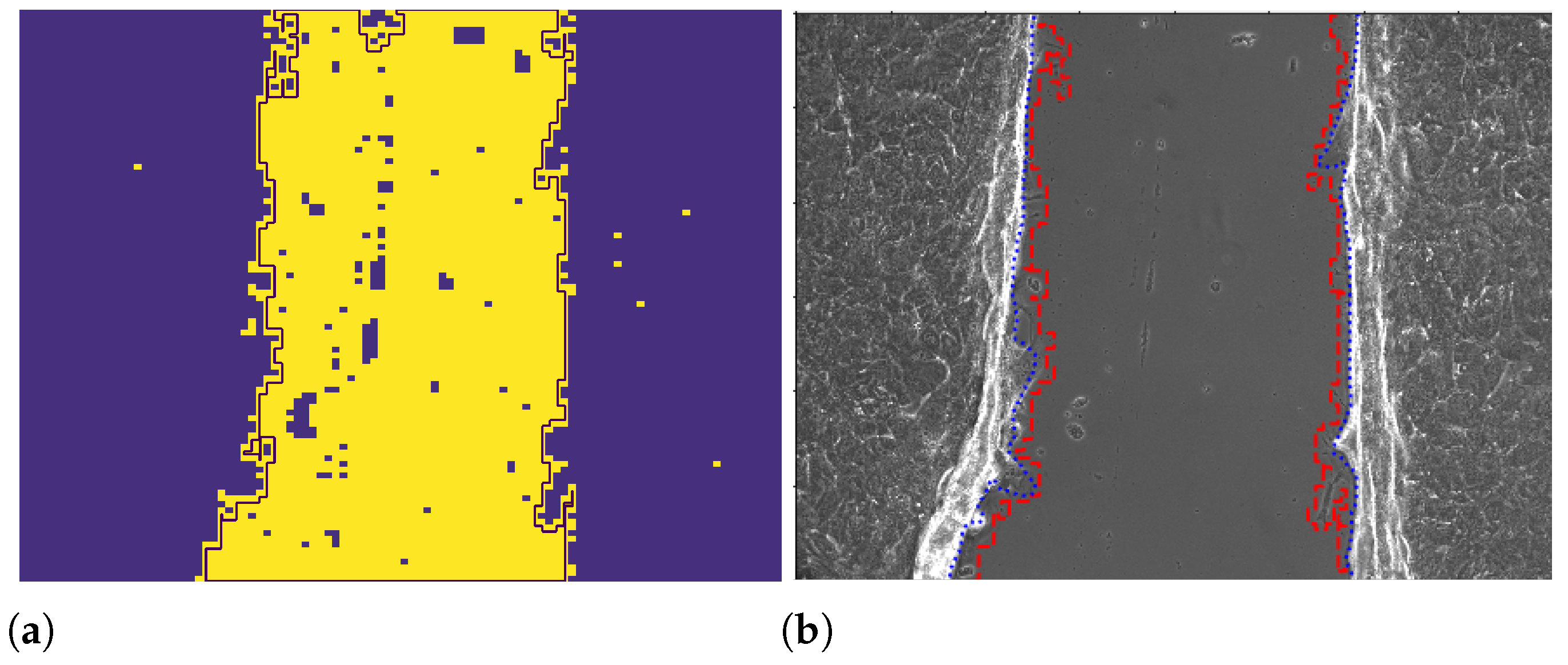
2.2.3. Wound Edge Recognition from Binarized Images
2.2.4. Wound Edge Recognition with the ImageJ Professional Tool
2.2.5. Wound Edge Recognition with Otsu Thresholding
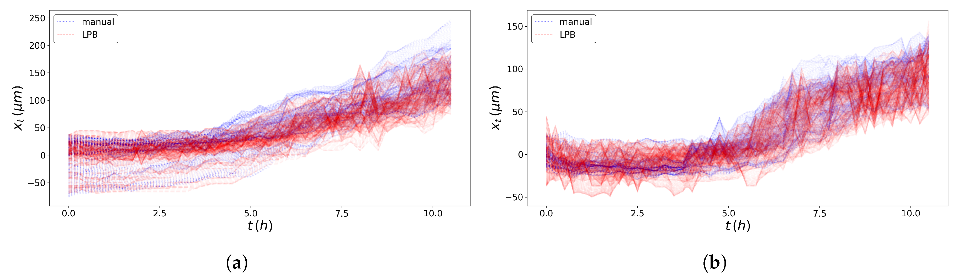
2.3. Pseudo-Particles’ Trajectories
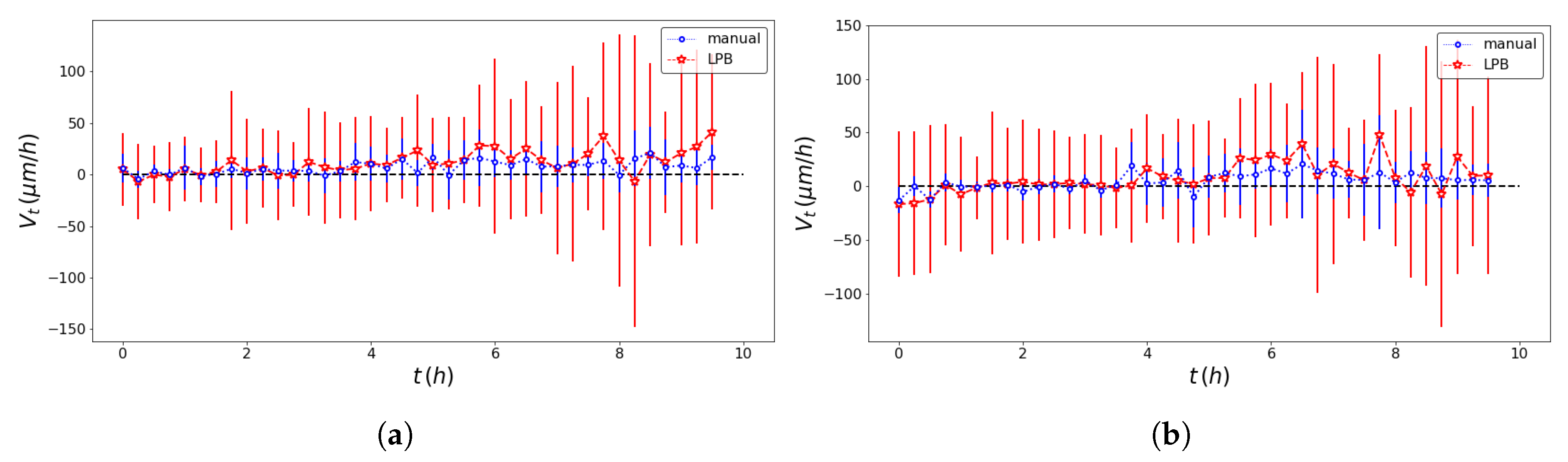
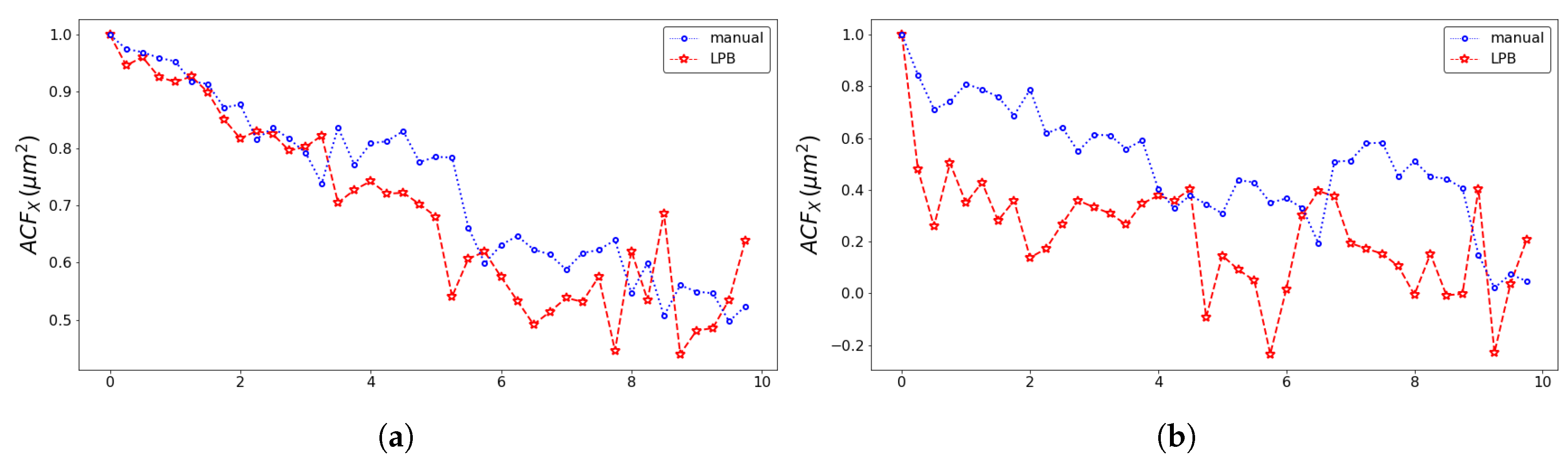
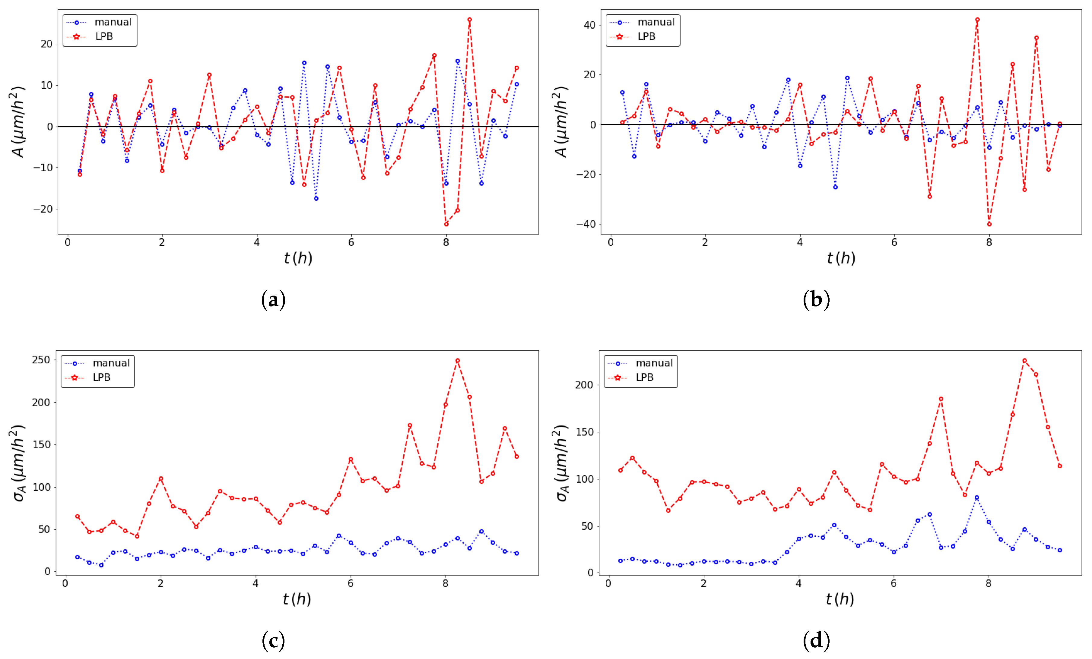
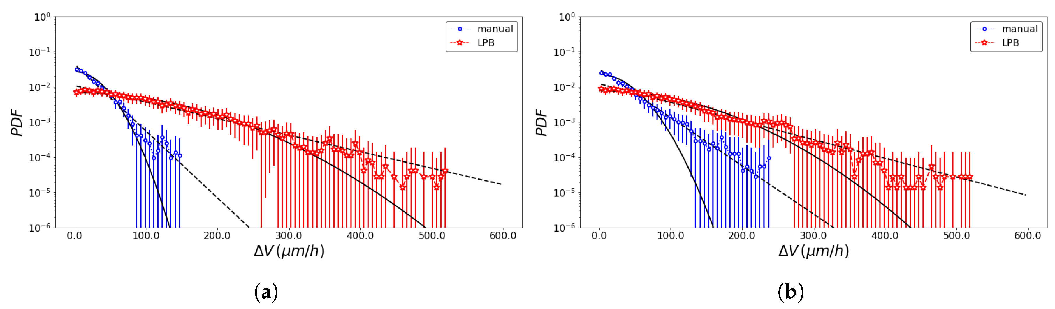
2.4. SPT Statistics
2.5. Fit Procedure
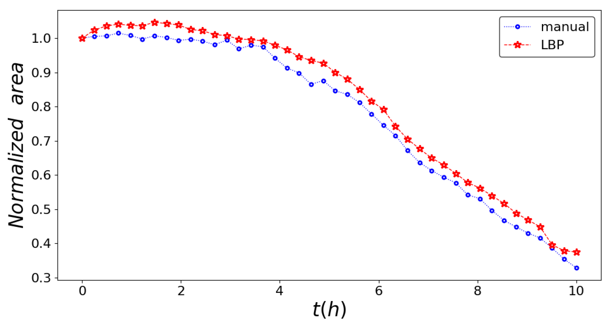
3. Results
4. Conclusions
Supplementary Materials
Author Contributions
Funding
Data Availability Statement
Acknowledgments
Conflicts of Interest
References
- Friedl, P.; Wolf, K. Tumour-cell invasion and migration: Diversity and escape mechanisms. Nat. Rev. Cancer 2003, 3, 362–374. [Google Scholar] [CrossRef] [PubMed]
- Rorth, P. Collective cell migration. Annu. Rev. Cell Dev. Biol. 2009, 25, 407–429. [Google Scholar] [CrossRef] [PubMed]
- Ladoux, B.; Mège, R.M. Mechanobiology of collective cell behaviours. Nat. Rev. Mol. Cell Biol. 2017, 18, 743–757. [Google Scholar] [CrossRef] [PubMed]
- Lintz, M.; Muñoz, A.; Reinhart-King, C.A. The Mechanics of Single Cell and Collective Migration of Tumor Cells. J. Biomech. Eng. 2017, 139, 0210051–0210059. [Google Scholar] [CrossRef] [PubMed]
- Hakim, V.; Silberzan, P. Collective cell migration: A physics perspective. Rep. Prog. Phys. 2017, 80, 076601. [Google Scholar] [CrossRef] [PubMed]
- Ascione, F.; Vasaturo, A.; Caserta, S.; D’Esposito, V.; Formisano, P.; Guido, S. Comparison between fibroblast wound healing and cell random migration assays in vitro. Exp. Cell Res. 2008, 347, 123–132. [Google Scholar] [CrossRef] [PubMed]
- Te Boekhorst, V.; Preziosi, L.; Friedl, P. Plasticity of cell migration in vivo and in silico. Annu. Rev. Cell Dev. Biol. 2016, 32, 491–526. [Google Scholar] [CrossRef] [PubMed]
- Thuroff, F.; Goychuk, A.; Reiter, M.; Frey, E. Bridging the gap between single-cell migration and collective dynamics. eLife 2019, 8, e46842. [Google Scholar] [CrossRef] [PubMed]
- Zheng, C.; Yu, Z.; Zhou, Y.; Tao, L.; Pang, Y.; Chen, T.; Zhang, X.; Qiu, H.; Zhou, H.; Chen, Z.; et al. Live cell imaging analysis of the epigenetic regulation of the human endothelial cell migration at single-cell resolution. Lab Chip 2012, 12, 3063–3072. [Google Scholar] [CrossRef]
- Dieterich, P.; Klages, R.; Preuss, R.; Schwab, A. Anomalous dynamics of cell migration. Proc. Natl. Acad. Sci. USA 2008, 105, 459–463. [Google Scholar] [CrossRef] [PubMed]
- Souza Vilela Podestá, T.; Venzel Rosembach, T.; Aparecida dos Santos, A.; Lobato Martins, M. Anomalous diffusion and q-Weibull velocity distributions in epithelial cell migration. PLoS ONE 2017, 12, e0180777. [Google Scholar] [CrossRef] [PubMed]
- Luzhansky, I.D.; Schwartz, A.D.; Cohen, J.D.; MacMunn, J.P.; Barney, L.E.; Jansen, L.E.; Peyton, S.R. Anomalously diffusing and persistently migrating cells in 2D and 3D culture environments. APL Bioeng. 2018, 2, 026112. [Google Scholar] [CrossRef] [PubMed]
- Otsu, N. A Threshold Selection Method from Gray-Level Histograms. IEEE Trans. Syst. Man Cybern. 1979, 9, 62–66. [Google Scholar] [CrossRef]
- Rasband, W.S. ImageJ; U.S. National Institutes of Health: Bethesda, MD, USA, 1997–2018. Available online: https://imagej.nih.gov/ij/ (accessed on 1 November 2020).
- Zuiderveld, K. Contrast limited adaptive histogram equalization. In Graphics Gems IV; Heckbert, P., Ed.; Academic Press: Cambridge, MA, USA, 1994; pp. 474–485. [Google Scholar]
- Python Library OpenCV-Python. Available online: https://OpenCV-python-tutroals.readthedocs.io/en/ (accessed on 1 November 2020).
- Python Library Scikit-Image. Available online: https://scikit-image.org (accessed on 1 November 2020).
- Jolliffe, I.T.; Cadima, J. Principal component analysis: A review and recent developments. Philos. Trans. R. Soc. A 2016, 374, 20150202. [Google Scholar] [CrossRef]
- Python Library Scikit-Learn. Available online: https://scikit-learn.org (accessed on 1 November 2020).
- Python Library Scipy. Available online: https://www.scipy.org/ (accessed on 1 November 2020).


| Model | Front | Method | SD (m/h) | SD (h) | Adj. R-Squared |
|---|---|---|---|---|---|
| L | ImageJ | 0.990 | |||
| L | texture analysis | 0.984 | |||
| R | ImageJ | 0.987 | |||
| R | texture analysis | 0.975 |
| Model | Front | Method | SD (m) | SD (m) | Adj. R-Squared |
|---|---|---|---|---|---|
| L | ImageJ | ||||
| L | texture analysis | ||||
| R | ImageJ | ||||
| R | texture analysis | ||||
| L | ImageJ | ||||
| L | texture analysis | ||||
| R | ImageJ | ||||
| R | texture analysis |
| Front | Variable | Pearson’s Coeff. | p-Value |
|---|---|---|---|
| L | x-coords | 0.942 | 0.0 |
| y-coords | 0.985 | 0.0 | |
| 0.997 | 1 × 10 | ||
| 0.547 | 1 × 10 | ||
| 0.275 | 0.08 | ||
| R | x-coords | 0.913 | 0.0 |
| y-coords | 0.986 | 0.0 | |
| 0.997 | 1 × 10 | ||
| 0.630 | 1 × 10 | ||
| 0.156 | 0.19 |
Publisher’s Note: MDPI stays neutral with regard to jurisdictional claims in published maps and institutional affiliations. |
© 2021 by the authors. Licensee MDPI, Basel, Switzerland. This article is an open access article distributed under the terms and conditions of the Creative Commons Attribution (CC BY) license (http://creativecommons.org/licenses/by/4.0/).
Share and Cite
Scheda, R.; Vitali, S.; Giampieri, E.; Pagnini, G.; Zironi, I. Study of Wound Healing Dynamics by Single Pseudo-Particle Tracking in Phase Contrast Images Acquired in Time-Lapse. Entropy 2021, 23, 284. https://doi.org/10.3390/e23030284
Scheda R, Vitali S, Giampieri E, Pagnini G, Zironi I. Study of Wound Healing Dynamics by Single Pseudo-Particle Tracking in Phase Contrast Images Acquired in Time-Lapse. Entropy. 2021; 23(3):284. https://doi.org/10.3390/e23030284
Chicago/Turabian StyleScheda, Riccardo, Silvia Vitali, Enrico Giampieri, Gianni Pagnini, and Isabella Zironi. 2021. "Study of Wound Healing Dynamics by Single Pseudo-Particle Tracking in Phase Contrast Images Acquired in Time-Lapse" Entropy 23, no. 3: 284. https://doi.org/10.3390/e23030284
APA StyleScheda, R., Vitali, S., Giampieri, E., Pagnini, G., & Zironi, I. (2021). Study of Wound Healing Dynamics by Single Pseudo-Particle Tracking in Phase Contrast Images Acquired in Time-Lapse. Entropy, 23(3), 284. https://doi.org/10.3390/e23030284