
A New Pooling Approach Based on Zeckendorf’s Theorem for Texture Transfer Information


Abstract
1. Introduction
2. Related Works
2.1. Pooling Strategies in Image Processing
2.2. Pooling and Statistics
2.3. Texture Coding
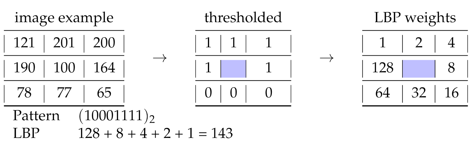
3. Z Representation
3.1. Zeckendorf Additive Partition
| Algorithm 1: Image Z coding. |
 |
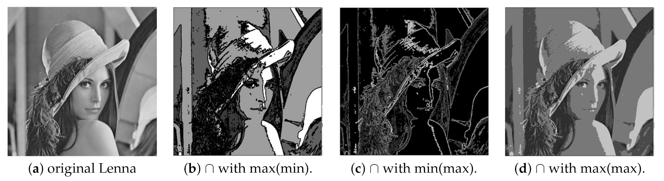
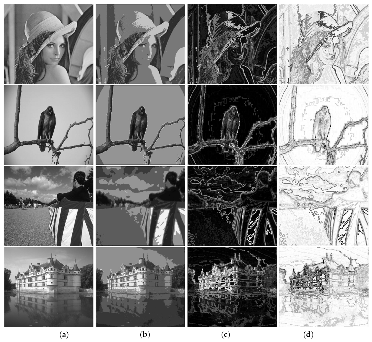
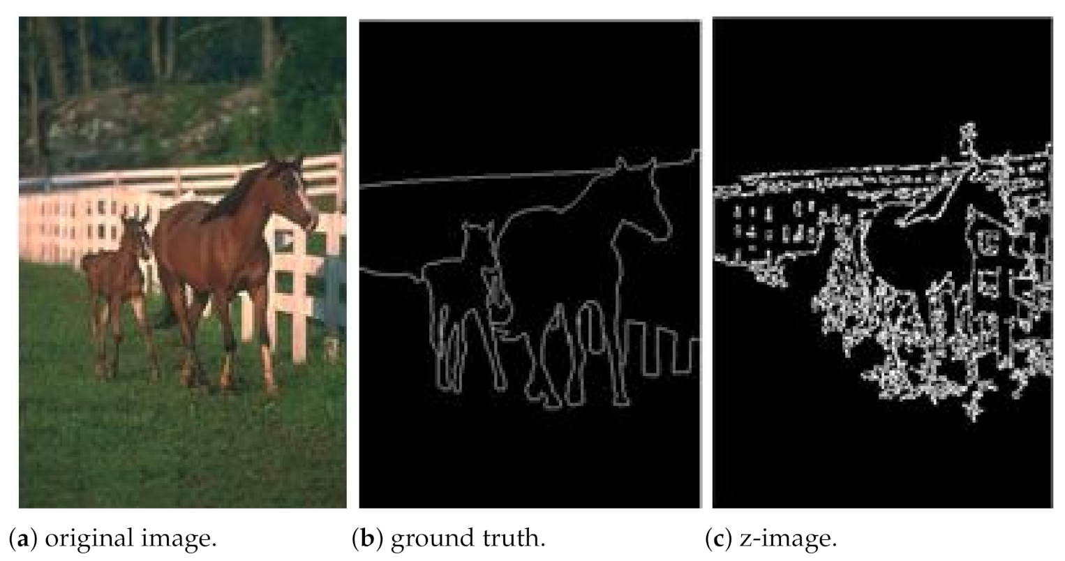
3.2. Evaluation and Result for Segmentation
4. Z Pooling
5. Numerical Evaluation with CNN
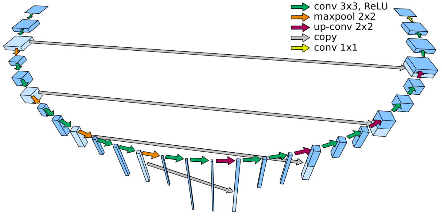
5.1. Implementation
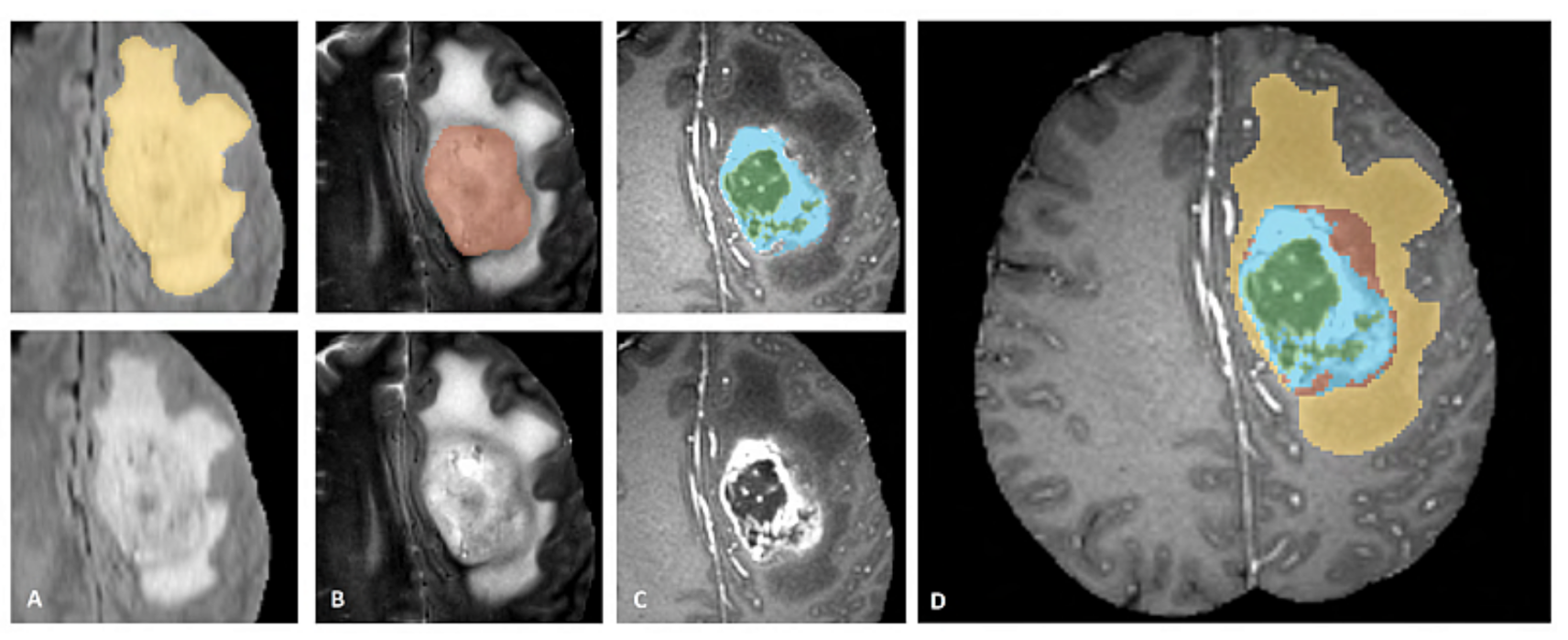
5.2. Miccai BraTS Dataset
5.3. Experiment Details
5.3.1. Data
5.3.2. Training Protocol
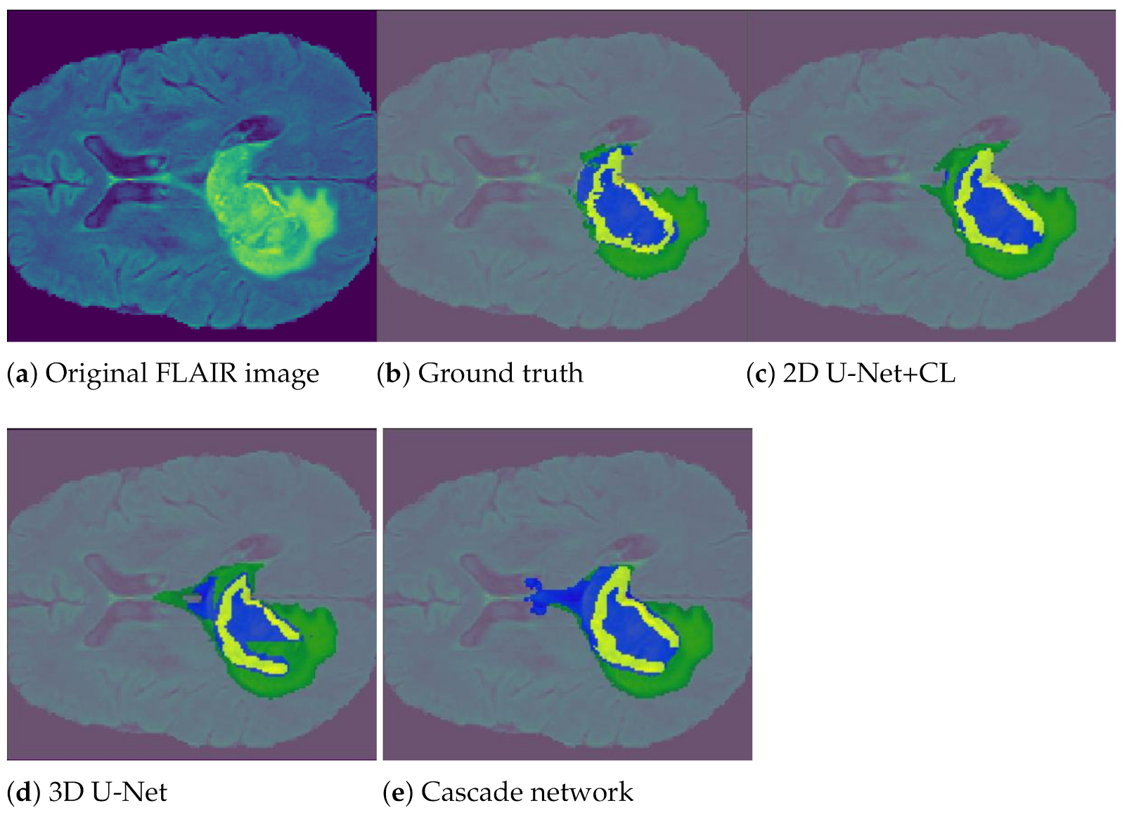
5.3.3. Results and Discussion
6. Conclusions
Author Contributions
Funding
Institutional Review Board Statement
Informed Consent Statement
Data Availability Statement
Acknowledgments
Conflicts of Interest
References
- Shen, D.; Wu, G.; Suk, H. Deep Learning in Medical Image Analysis. Annu. Rev. Biomed. Eng. 2017, 19, 221–248. [Google Scholar] [CrossRef] [PubMed]
- Serre, T.; Wolf, L.; Poggio, T. Object Recognition with Features Inspired by Visual Cortex. In Proceedings of the 2005 IEEE Computer Society Conference on Computer Vision and Pattern Recognition (CVPR’05), San Diego, CA, USA, 20–25 June 2005; Volume 2, pp. 994–1000. [Google Scholar] [CrossRef]
- Arel, I.; Rose, D.; Karnowski, T. Deep Machine Learning—A New Frontier in Artificial Intelligence Research [Research Frontier]. IEEE Comp. Int. Mag. 2010, 5, 13–18. [Google Scholar] [CrossRef]
- Goodfellow, I.; Bengio, Y.; Courville, A. Deep Learning; MIT Press: Cambridge, MA, USA, 2016. [Google Scholar]
- Yu, D.; Wang, H.; Chen, P.; Wei, Z. Mixed Pooling for Convolutional Neural Networks. In Proceedings of the International Conference on Rough Sets and Knowledge Technology, Shanghai, China, 24–26 October 2014; pp. 364–375. [Google Scholar]
- Lee, C.; Gallagher, P.; Tu, Z. Generalizing Pooling Functions in Convolutional Neural Networks: Mixed, Gated, and Tree. In Proceedings of the 19th International Conference on Artificial Intelligence and Statistics, San Diego, CA, USA, 9–12 May 2015. [Google Scholar]
- Lazebnik, S.; Schmid, C.; Ponce, J. Beyond Bags of Features: Spatial Pyramid Matching for Recognizing Natural Scene Categories. In Proceedings of the IEEE Computer Society Conference on Computer Vision and Pattern Recognition, New York, NY, USA, 12–17 June 2006; Volume 2, pp. 2169–2178. [Google Scholar] [CrossRef]
- Haralick, R. Statistical and Structural Approaches to Texture. Proc. IEEE 1979, 67, 786–804. [Google Scholar] [CrossRef]
- Li, C.; Zhang, Y.; Xie, E.Y. When an attacker meets a cipher-image in 2018: A year in review. J. Inf. Secur. Appl. 2019, 48, 102361. [Google Scholar] [CrossRef]
- Yu, F.; Koltun, V. Multi-Scale Context Aggregation by Dilated Convolutions. In Proceedings of the International Conference on Learning Representations (ICLR), San Juan, Puerto Rico, 2–4 May 2016. [Google Scholar]
- Yang, M.; Yu, K.; Zhang, C.; Li, Z.; Yang, K. DenseASPP for Semantic Segmentation in Street Scenes. In Proceedings of the IEEE Conference on Computer Vision and Pattern Recognition (CVPR), Salt Lake City, UT, USA, 18–23 June 2018. [Google Scholar]
- Scherer, D.; Müller, A.; Behnke, S. Evaluation of Pooling Operations in Convolutional Architectures for Object Recognition. In Proceedings of the 20th International Conference on Artificial Neural Networks: Part III; ICANN’10; Springer: Berlin/Heidelberg, Germany, 2010; pp. 92–101. [Google Scholar]
- Sharma, S.; Rajesh, M. Implications of Pooling Strategies in Convolutional Neural Networks: A Deep Insight. Found. Comput. Decis. Sci. 2019, 44, 303–330. [Google Scholar] [CrossRef]
- Gulcehre, C.; Cho, K.; Pascanu, R.; Bengio, Y. Learned-Norm Pooling for Deep Feedforward and Recurrent Neural Networks. In Proceedings of the European Conference on Machine Learning and Knowledge Discovery in Databases, Nancy, France, 15–19 September 2014; pp. 530–546. [Google Scholar] [CrossRef]
- Agostinelli, F.; Hoffman, M.; Sadowski, P.; Baldi, P. Learning Activation Functions to Improve Deep Neural Networks. arXiv 2014, arXiv:1412.6830. [Google Scholar]
- Boureau, Y.L.; Ponce, J.; Lecun, Y. A Theoretical Analysis of Feature Pooling in Visual Recognition. In Proceedings of the 27th International Conference on Machine Learning, Haifa, Israel, 21–25 June 2010; pp. 111–118. [Google Scholar]
- Sheskin, D.J. Handbook of Parametric and Nonparametric Statistical Procedures, 4th ed.; Chapman & Hall/CRC: Boca Raton, FL, USA, 2007. [Google Scholar]
- Howell, D. Statistical Methods for Psychology, 6th ed.; Thomson: Belmont, CA, USA, 2007. [Google Scholar]
- Lowe, D.G. Object Recognition from Local Scale-Invariant Fea- tures. In Proceedings of the IEEE Computer Society Conference on Computer Vision and Pattern Recognition, Fort Collins, CO, USA, 23–25 June 1999; Volume 2, pp. 1150–1157. [Google Scholar]
- Moorthy, A.; Bovik, A. Visual Importance Pooling for Image Quality Assessment. IEEE J. Sel. Top. Signal Process. 2009, 3, 193–201. [Google Scholar] [CrossRef]
- Pietikinen, M.; Hadid, A.; Zhao, G.; Ahonen, T. Computer Vision Using Local Binary Patterns; Computer Imaging and Vision; Springer: Berlin/Heidelberg, Germany, 2011; Volume 40. [Google Scholar]
- Ojala, T.; Pietikäinen, M.; Harwood, D. A comparative study of texture measures with classification based on feature distributions. Pattern Recognit. 1996, 29, 51–59. [Google Scholar] [CrossRef]
- Tan, X.; Triggs, B. Enhanced Local Texture Feature Sets for Face Recognition Under Difficult Lighting Conditions. In Analysis and Modeling of Faces and Gestures; Lecture Notes in Computer Science; Springer: Berlin/Heidelberg, Germany, 2007; Volume 4778, pp. 235–249. [Google Scholar]
- Zeckendorf, E. Représentation des nombres naturels par une somme de nombres de Fibonacci ou de nombres de Lucas. Bull. Soc. Roy. Sci. Liege 1972, 41, 179–182. [Google Scholar]
- Vigneron, V.; Syed, T.; Duarte, L.; Lang, E.; Behlim, S.; Tomé, A. Z-Images. In Proceedings of the 7th Iberian Conference on Pattern Recognition and Image Analysis, Faro, Portugal, 20–23 June 2017; pp. 177–184. [Google Scholar]
- Yao, C.; Chen, S. Color texture retrieval, color texture segmentation, content-based retrieval, images, local edge pattern, similarity measure, texture, texture region. Pattern Recognit. 2003, 36, 913–929. [Google Scholar] [CrossRef]
- Kellokumpu, V.; Zhao, G.; Li, S.Z.; Pietikäinen, M. Dynamic Texture Based Gait Recognition. In Proceedings of the International Conference on Biometrics, Alghero, Italy, 2–5 June 2009; pp. 1000–1009. [Google Scholar]
- Wang, H.; Ullah, M.; Klaser, A.; Laptev, I.; Schmid, C. Evaluation of Local Spatio-temporal Features for Action Recognition. In Proceedings of the British Machine Vision Conference, London, UK, 7–10 September 2009; Volume 124. [Google Scholar]
- Chen, J.; Zhao, G.; Pietikäinen, M. An Improved Local Descriptor and Threshold Learning for Unsupervised Dynamic Texture Segmentation. In Proceedings of the 2nd IEEE International Workshop on Machine Learning for Vision-based Motion Analysis (MLVMA09), Kyoto, Japan, 28 September 2009; IEEE: Kyoto, Japan, 2009; pp. 460–467. [Google Scholar]
- Stone, Z.; Zickler, T.; Darrell, T. Autotagging Facebook: Social Network Context Improves Photo Annotation. In Proceedings of the Computer Vision and Pattern Recognition Workshops, Anchorage, AK, USA, 23–28 June 2008; pp. 1–8. [Google Scholar] [CrossRef]
- Fowlkes, C.; Martin, D.; Malik, J. Learning Affinity Functions for Image Segmentation: Combining Patch-based and Gradient-based Approaches. In Proceedings of the 2003 IEEE Computer Society Conference on Computer Vision and Pattern Recognition, Madison, WI, USA, 18–20 June 2003; Volume 2, pp. 2–54. [Google Scholar] [CrossRef]
- Shelhamer, E.; Long, J.; Darrell, T. Fully Convolutional Networks for Semantic Segmentation. IEEE Trans. Pattern Anal. Mach. Intell. 2017, 39, 640–651. [Google Scholar] [CrossRef] [PubMed]
- Wang, G.; Li, W.; Ourselin, S.; Vercauteren, T. Automatic Brain Tumor Segmentation Using Cascaded Anisotropic Convolutional Neural Networks. In Brainlesion: Glioma, Multiple Sclerosis, Stroke and Traumatic Brain Injuries; Lecture Notes in Computer Science; Springer: Berlin/Heidelberg, Germany, 2018; Volume 10670 LNCS, pp. 178–190. [Google Scholar] [CrossRef]
- Menze, B. The multimodal brain tumor image segmentation benchmark (BRATS). IEEE Trans. Med Imaging 2014, 34, 1993–2024. [Google Scholar] [CrossRef] [PubMed]
- Razzak, M.; Naz, S.; Zaib, A. Deep Learning for Medical Image Processing: Overview, Challenges and the Future. In Classification in BioApps; Springer: Berlin/Heidelberg, Germany, 2018; pp. 323–350. [Google Scholar]
- Menze, B.H.; Jakab, A.; Bauer, S.; Kalpathy-Cramer, J.; Farahani, K.; Kirby, J.; Burren, Y.; Porz, N.; Slotboom, J.; Wiest, R.; et al. The multimodal brain tumor image segmentation benchmark (BRATS). IEEE Trans. Med. Imaging 2015, 34, 1993–2024. [Google Scholar] [CrossRef] [PubMed]
- Bengio, Y.; Louradour, J.; Collobert, R.; Weston, J. Curriculum Learning. In Proceedings of the 26th Annual International Conference on Machine Learning, Montreal, QC, Canada, 14–18 June 2009; pp. 41–48. [Google Scholar]
- Ronneberger, O.; Fischer, P.; Brox, T. U-net: Convolutional Networks for Biomedical Image Segmentation. In Proceedings of the International Conference on Medical Image Computing and Computer-Assisted Intervention, Munich, Germany, 5–9 October 2015; pp. 234–241. [Google Scholar]
- Dong, H.; Yang, G.; Liu, F.; Mo, Y.; Guo, Y. Automatic Brain Tumor Detection and Segmentation Using U-Net Based Fully Convolutional Networks. In Proceedings of the Annual Conference on Medical Image Understanding and Analysis, Edinburgh, UK, 11–13 July 2017; pp. 506–517. [Google Scholar]
- Çiçek, Ö; Abdulkadir, A.; Lienkamp, S.S.; Brox, T.; Ronneberger, O. 3D U-Net: Learning Dense Volumetric Segmentation from Sparse Annotation. In Proceedings of the International Conference on Medical Image Computing and Computer-Assisted Intervention, Athens, Greece, 17–21 October 2016; pp. 424–432. [Google Scholar]
- Clevert, D.A.; Unterthiner, T.; Hochreiter, S. Fast and Accurate Deep Network Learning by Exponential Linear Units (ELUs). In Proceedings of the 4th International Conference on Learning Representations, San Diego, CA, USA, 7–9 May 2015. [Google Scholar]


| Rank | Algorithm | Average Recall | Average Precision | Average F-Measure |
|---|---|---|---|---|
| 1 | gPb-UCM | 0.7397 | 0.7241 | 0.7226 |
| 2 | Global Probability of Boundary (GPB) | 0.7261 | 0.6902 | 0.7031 |
| 3 | Ren | 0.7198 | 0.6959 | 0.7019 |
| 4 | Z-coding | 0.833 | 0.5875 | 0.6652 |
| 5 | Brightness/Texture Gradients (BTG) | 0.6999 | 0.637 | 0.6592 |
| 6 | Boosted Edge Learning (BEL) | 0.699 | 0.6254 | 0.6557 |
| 7 | Brightness Gradient (BG) | 0.6946 | 0.6011 | 0.6348 |
| 8 | Multiscale Gradient Magnitude (MGM) | 0.6562 | 0.5939 | 0.6133 |
| 9 | Gradient Magnitude (GM) | 0.6961 | 0.5677 | 0.6119 |
| 10 | Texture Gradient (TG) | 0.6231 | 0.6053 | 0.6076 |
| 11 | Second order Moment Matrix (SMM) | 0.6501 | 0.5891 | 0.6042 |
| Indicators | Average Recall | Average Precision | Average F-Measure |
|---|---|---|---|
| Proposed vs. manual benchmark | 0.8326 | 0.2495 | 0.3675 |
| Method | Loss Function | Training Set Size | # of Trainable Parameters | Test Set Size | Epochs | Training Duration (Hours) |
|---|---|---|---|---|---|---|
| Cascaded Network | Dice Loss | 100 | n/a | 25 | 30 | 9 |
| 2D U-Net | Dice Loss | 100 | 31,032,451 | 25 | 300 | 13 |
| 3D U-Net | Dice Loss | 100 | 14,491,619 | 25 | 300 | 24 |
| DL Network | Dice Score | Recall | Precision | ||||||
|---|---|---|---|---|---|---|---|---|---|
| Z Pooling Config | ① | ② | ③ | ① | ② | ③ | ① | ② | ③ |
| Cascaded Network | 0.58 | 0.71 | 0.52 | 0.73 | 0.71 | 0.76 | 0.80 | 0.88 | 0.88 |
| 2D U-Net | 0.65 | 0.62 | 0.72 | 0.77 | 0.77 | 0.79 | 0.81 | 0.86 | 0.77 |
| 3D U-Net | 0.46 | 0.55 | 0.46 | 0.72 | 0.73 | 0.75 | 0.86 | 0.83 | 0.84 |
| 2D U-Net + CL | 0.68 | 0.73 | 0.77 | 0.77 | 0.76 | 0.80 | 0.80 | 0.81 | 0.87 |
| 2D U-net+DA | 0.67 | 0.75 | 0.62 | 0.77 | 0.76 | 0.82 | 0.81 | 0.83 | 0.78 |
| 2D U-Net + DA + CL | 0.65 | 0.68 | 0.53 | 0.78 | 0.77 | 0.80 | 0.82 | 0.90 | 0.88 |
| Majority Voting | 0.61 | 0.67 | 0.60 | 0.76 | 0.75 | 0.79 | 0.82 | 0.85 | 0.84 |
Publisher’s Note: MDPI stays neutral with regard to jurisdictional claims in published maps and institutional affiliations. |
© 2021 by the authors. Licensee MDPI, Basel, Switzerland. This article is an open access article distributed under the terms and conditions of the Creative Commons Attribution (CC BY) license (http://creativecommons.org/licenses/by/4.0/).
Share and Cite
Vigneron, V.; Maaref, H.; Syed, T.Q. A New Pooling Approach Based on Zeckendorf’s Theorem for Texture Transfer Information. Entropy 2021, 23, 279. https://doi.org/10.3390/e23030279
Vigneron V, Maaref H, Syed TQ. A New Pooling Approach Based on Zeckendorf’s Theorem for Texture Transfer Information. Entropy. 2021; 23(3):279. https://doi.org/10.3390/e23030279
Chicago/Turabian StyleVigneron, Vincent, Hichem Maaref, and Tahir Q. Syed. 2021. "A New Pooling Approach Based on Zeckendorf’s Theorem for Texture Transfer Information" Entropy 23, no. 3: 279. https://doi.org/10.3390/e23030279
APA StyleVigneron, V., Maaref, H., & Syed, T. Q. (2021). A New Pooling Approach Based on Zeckendorf’s Theorem for Texture Transfer Information. Entropy, 23(3), 279. https://doi.org/10.3390/e23030279