Author Contributions
Data curation, N.A.K.; Formal analysis, N.A.K.; Funding acquisition, F.S.A. and C.A.T.R.; Investigation, N.A.K. and M.S.; Methodology, N.A.K. and M.S.; Project administration, M.S.; Resources, F.S.A. and C.A.T.R., M.S.; Software, M.S.; Supervision, M.S.; Visualization, N.A.K.; Writing—original draft, N.A.K.; Writing—review and editing, F.S.A., C.A.T.R., M.S. All authors have read and agreed to the published version of the manuscript.
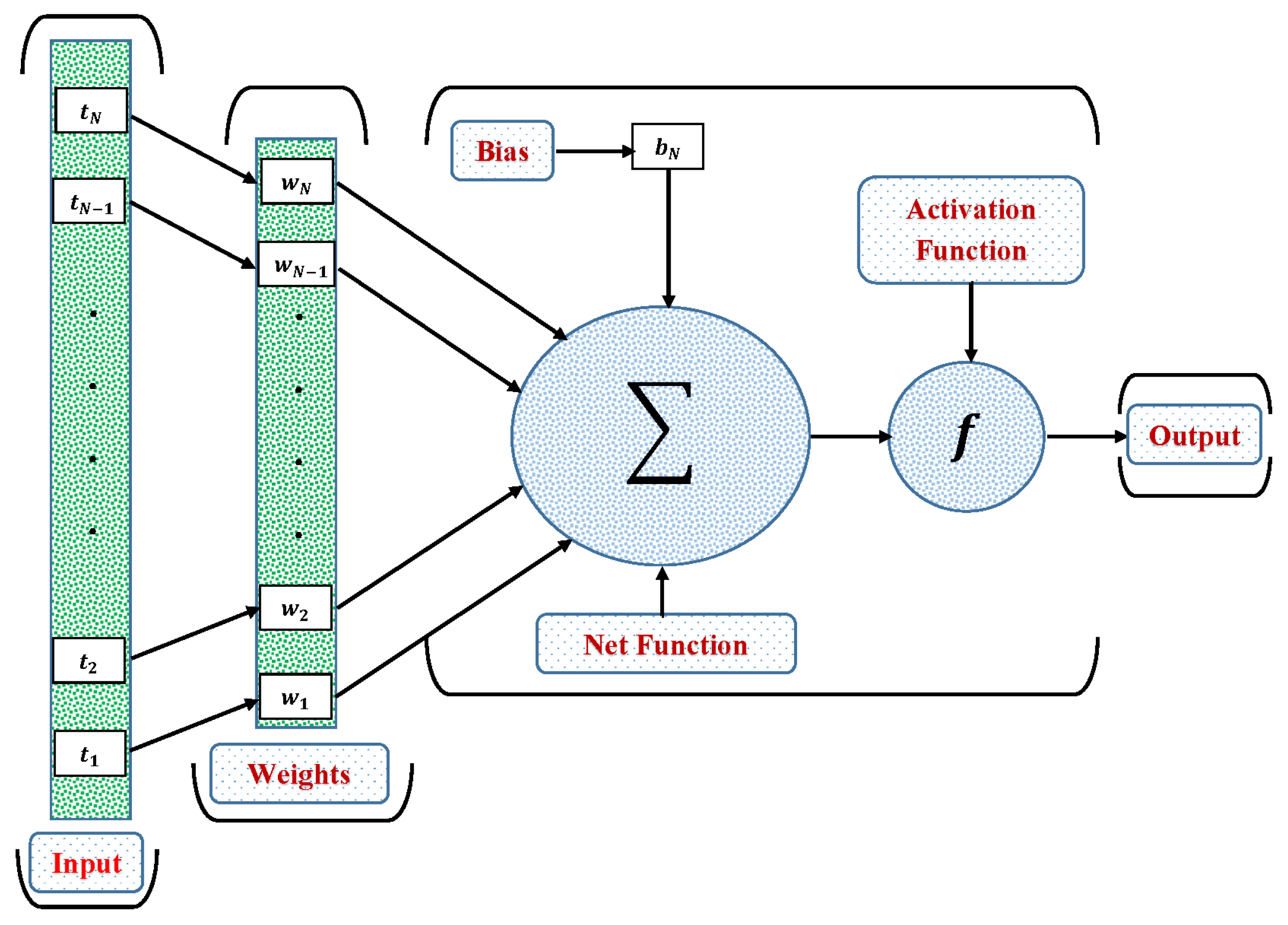
Figure 1.
Architecture of the basic ANN.
Figure 1.
Architecture of the basic ANN.
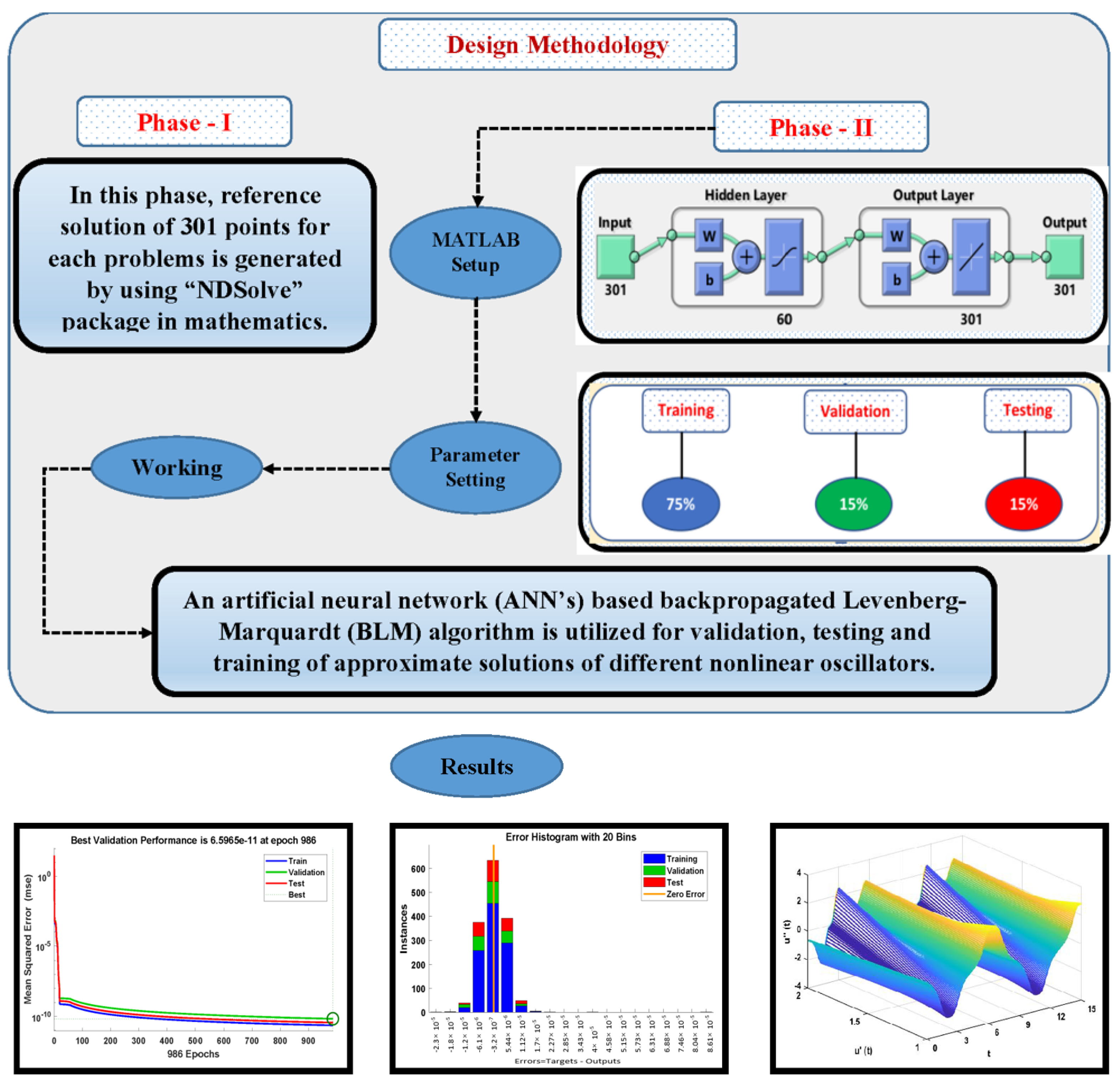
Figure 2.
Working mechanism of NN-BLMA for solving strongly nonlinear oscillators.
Figure 2.
Working mechanism of NN-BLMA for solving strongly nonlinear oscillators.
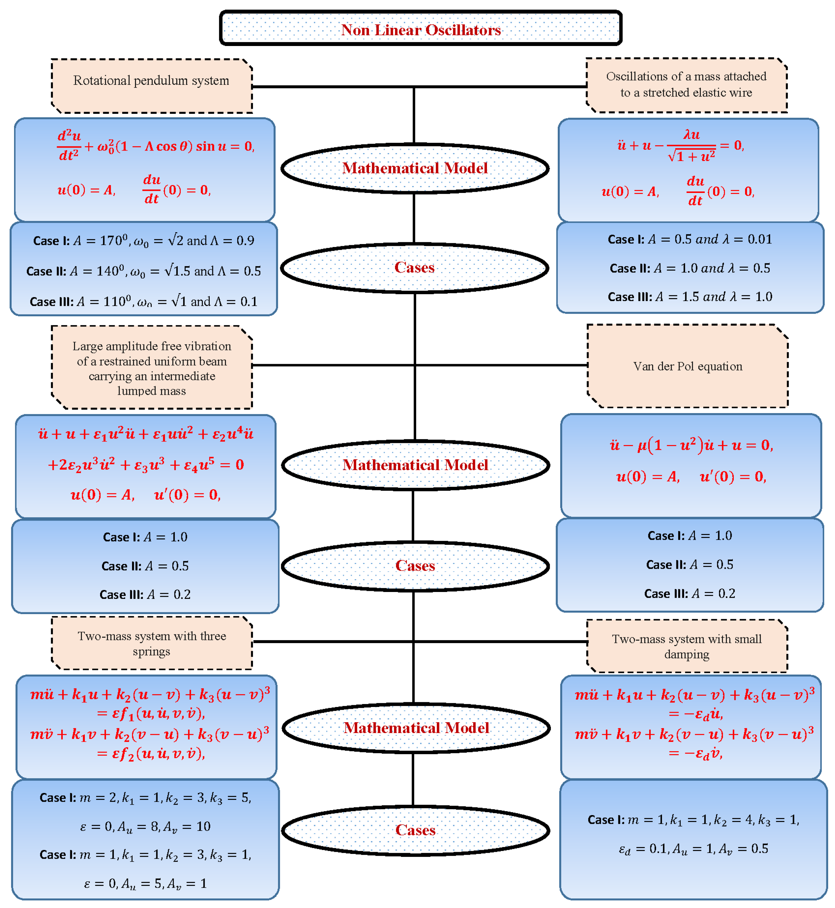
Figure 3.
A general view of different cases of nonlinear oscillators discussed in this paper.
Figure 3.
A general view of different cases of nonlinear oscillators discussed in this paper.
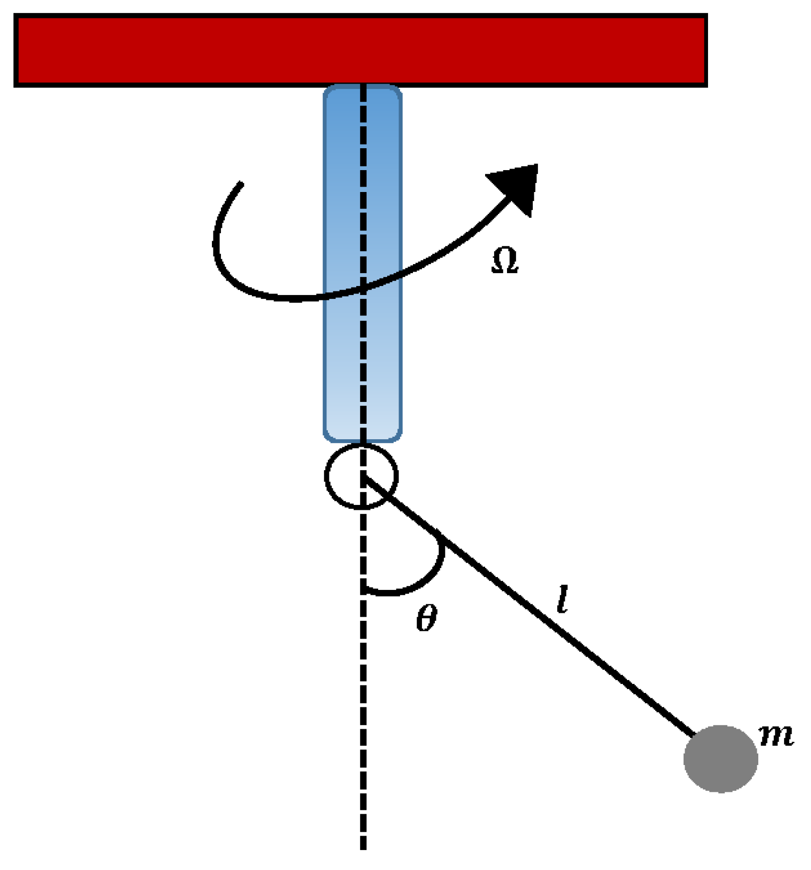
Figure 4.
A schematic of a rotational simple pendulum.
Figure 4.
A schematic of a rotational simple pendulum.
Figure 5.
(a) Approximate solutions by the design scheme for different cases of rotational pendulum system, while (b) illustrates the phase plane between velocity and displacement of the system.
Figure 5.
(a) Approximate solutions by the design scheme for different cases of rotational pendulum system, while (b) illustrates the phase plane between velocity and displacement of the system.
Figure 6.
Three-dimensional plots to study the influence of time in velocity and acceleration of rotational pendulum system.
Figure 6.
Three-dimensional plots to study the influence of time in velocity and acceleration of rotational pendulum system.
Figure 7.
Error histogram analysis for each case of rotational pendulum.
Figure 7.
Error histogram analysis for each case of rotational pendulum.
Figure 8.
Convergence of performance function in terms of MSE for each case of problem 1.
Figure 8.
Convergence of performance function in terms of MSE for each case of problem 1.
Figure 9.
Regression analysis for different cases of problem 1.
Figure 9.
Regression analysis for different cases of problem 1.
Figure 10.
Mass attached to the center of elastic wire.
Figure 10.
Mass attached to the center of elastic wire.
Figure 11.
(a) Approximate solutions obtained by proposed algorithm for the system. (b) shows the phase plane between velocity and displacement of the stretched elastic wire.
Figure 11.
(a) Approximate solutions obtained by proposed algorithm for the system. (b) shows the phase plane between velocity and displacement of the stretched elastic wire.
Figure 12.
Three-dimensional plots to study the influence of time in velocity and acceleration of mass attached to a stretched elastic wire.
Figure 12.
Three-dimensional plots to study the influence of time in velocity and acceleration of mass attached to a stretched elastic wire.
Figure 13.
Error histogram analysis for each case of mass attached to stretched elastic wire.
Figure 13.
Error histogram analysis for each case of mass attached to stretched elastic wire.
Figure 14.
Convergence of performance function in terms of mean square error for each case of problem 2.
Figure 14.
Convergence of performance function in terms of mean square error for each case of problem 2.
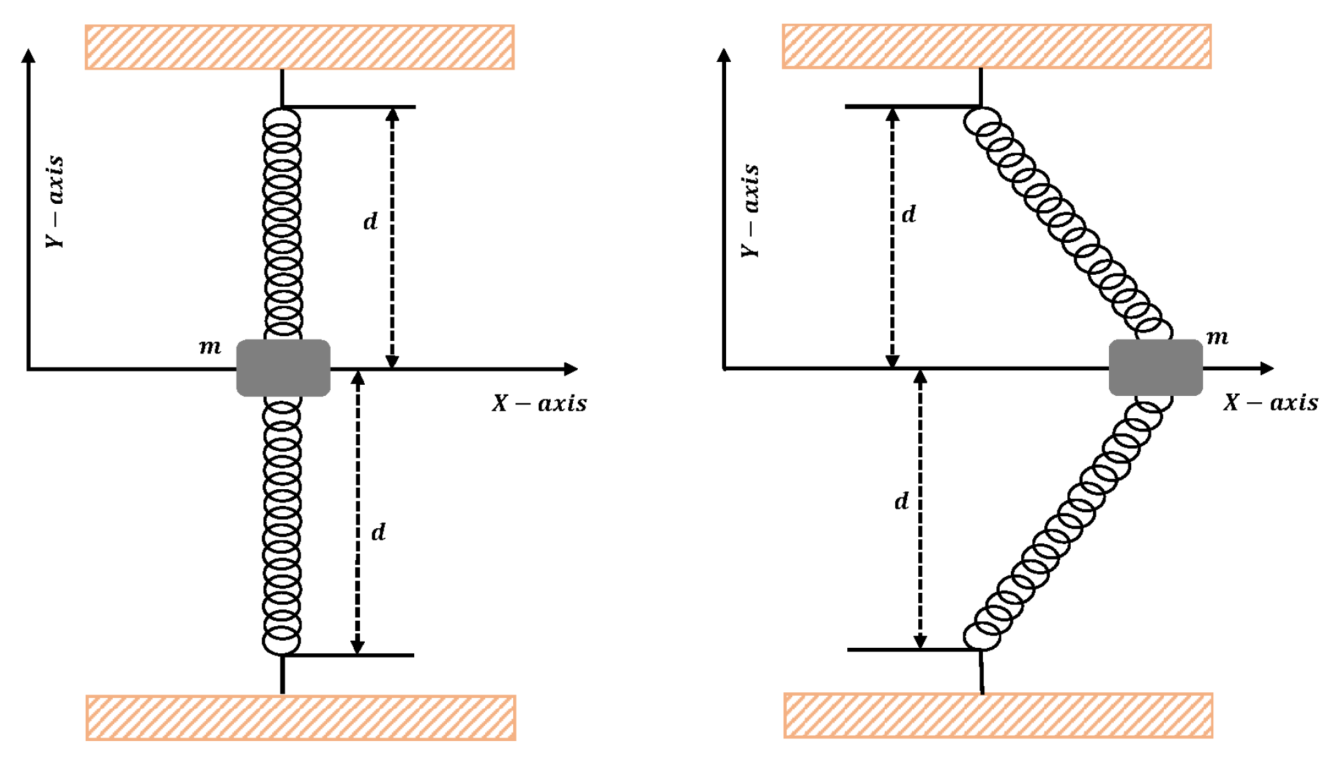
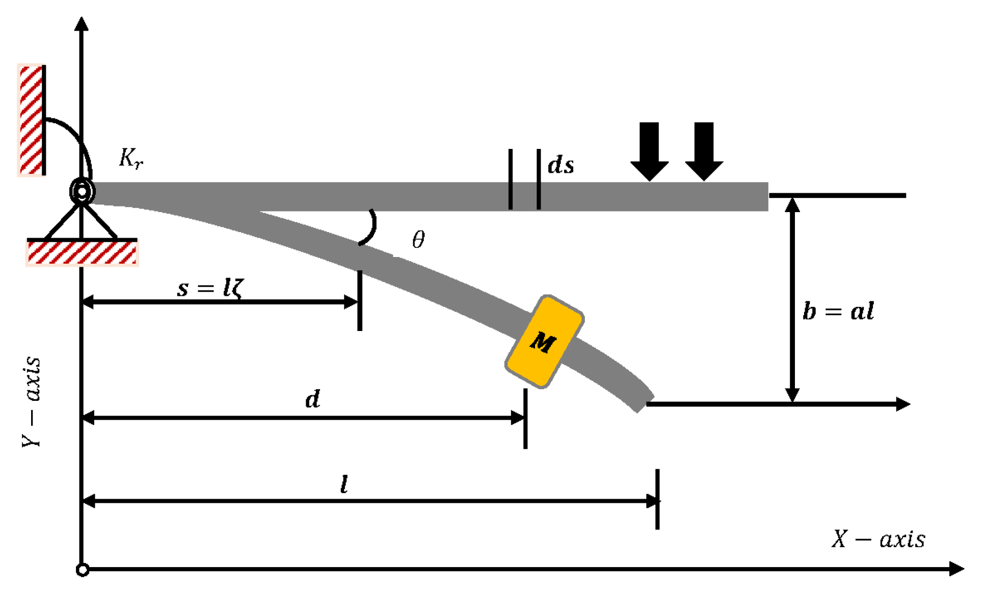
Figure 15.
Geometry and coordinate system for a beam with rotational spring and a lumped mass.
Figure 15.
Geometry and coordinate system for a beam with rotational spring and a lumped mass.
Figure 16.
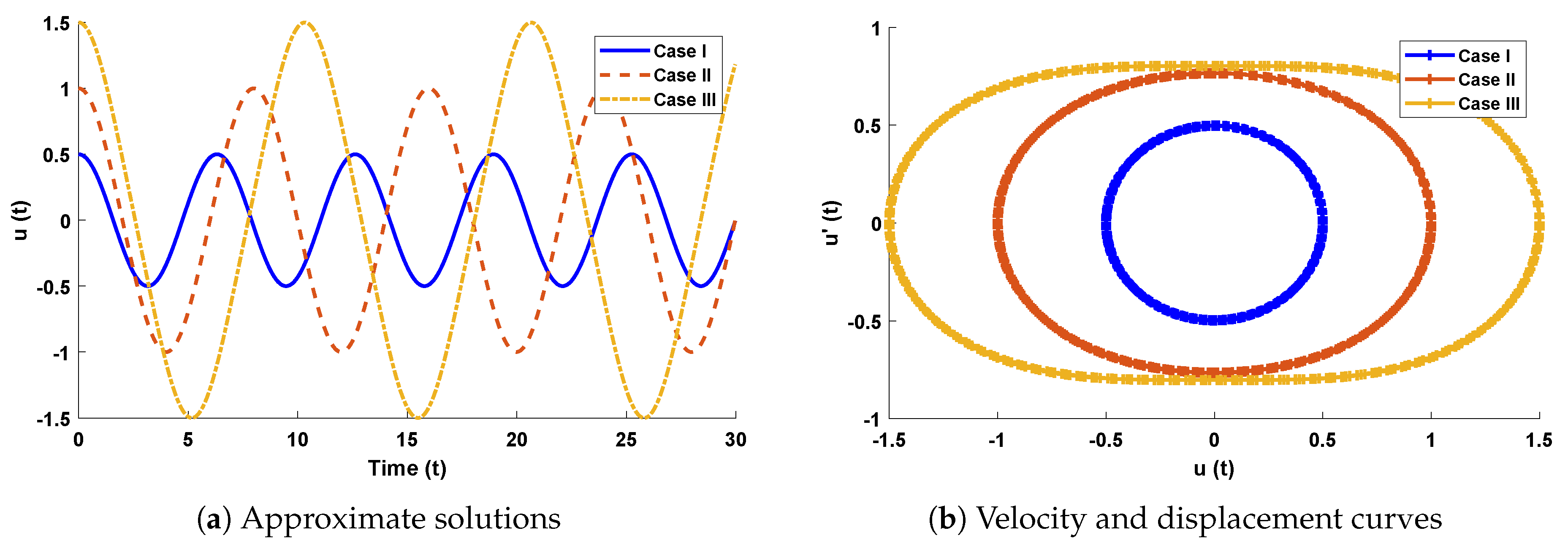
(a) Approximate solutions obtained by proposed algorithm for the system. (b) Phase plane analysis between velocity and displacement for mathematical model of restrained uniform beam carrying an intermediate lumped mass.
Figure 16.
(a) Approximate solutions obtained by proposed algorithm for the system. (b) Phase plane analysis between velocity and displacement for mathematical model of restrained uniform beam carrying an intermediate lumped mass.
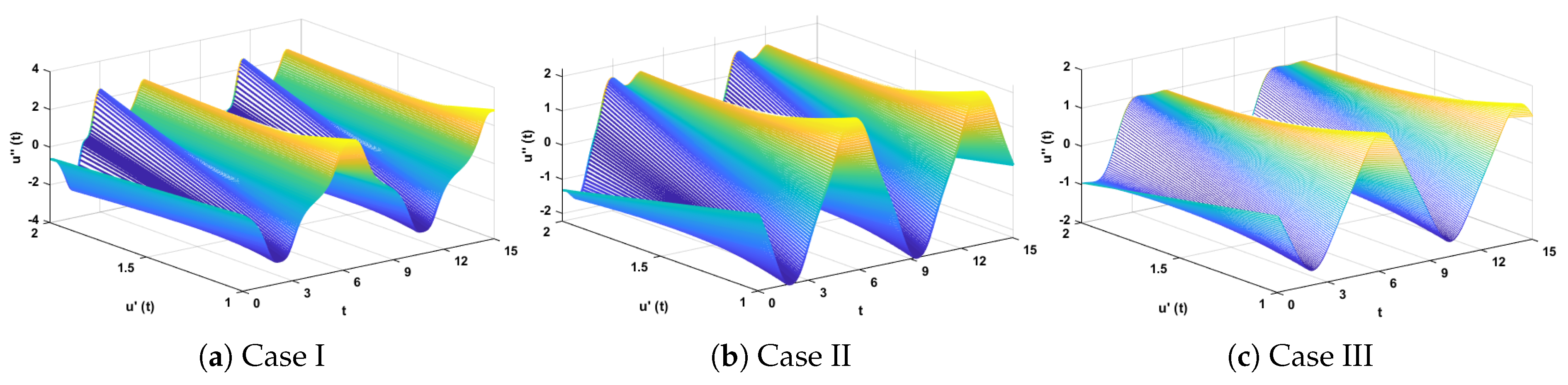
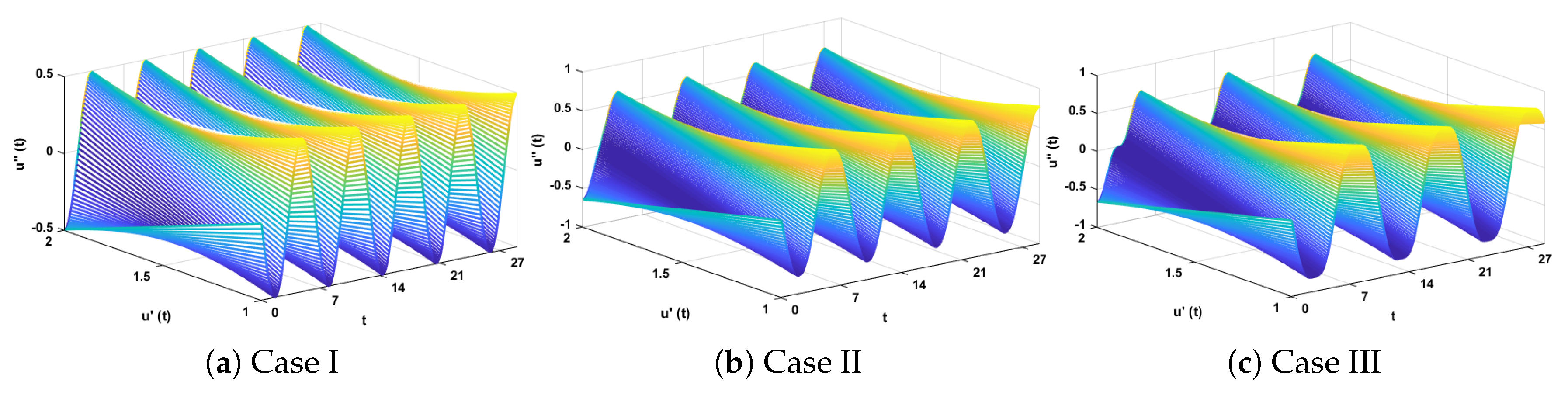
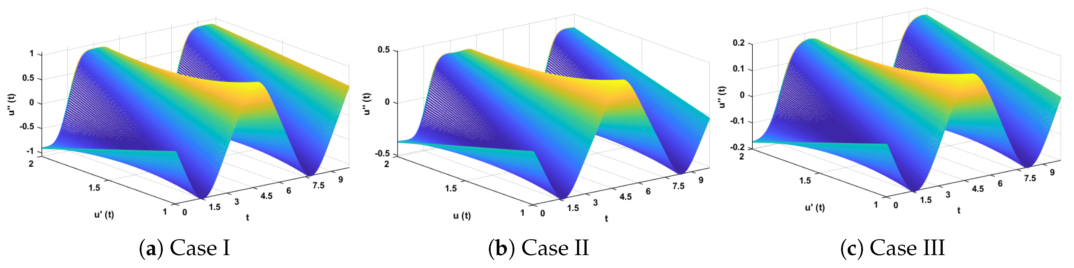
Figure 17.
Three-dimensional plots to study the influence of time in velocity and acceleration of mathematical model given in Equation (
6).
Figure 17.
Three-dimensional plots to study the influence of time in velocity and acceleration of mathematical model given in Equation (
6).
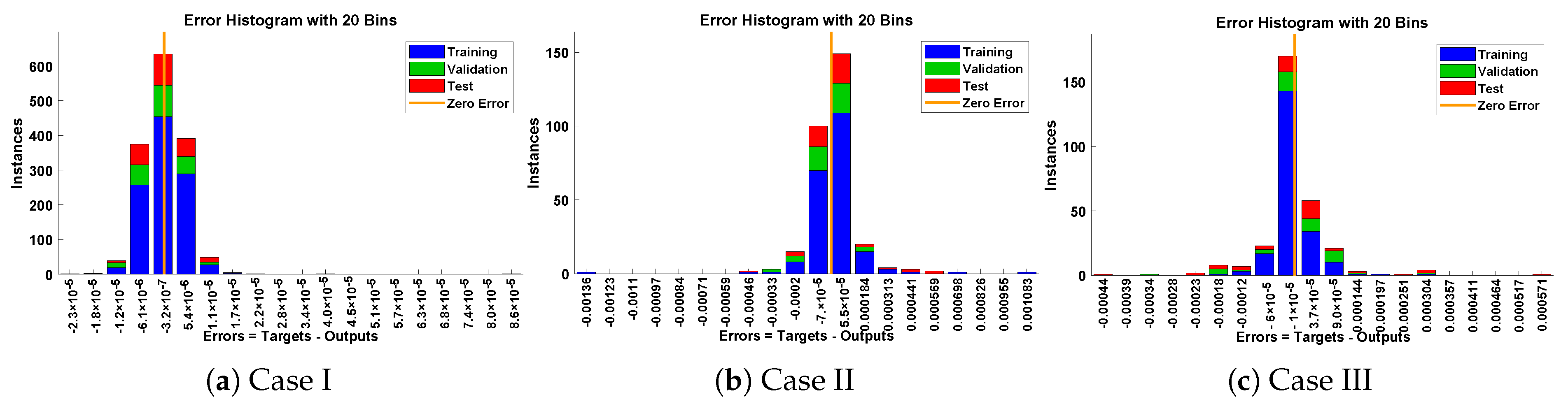
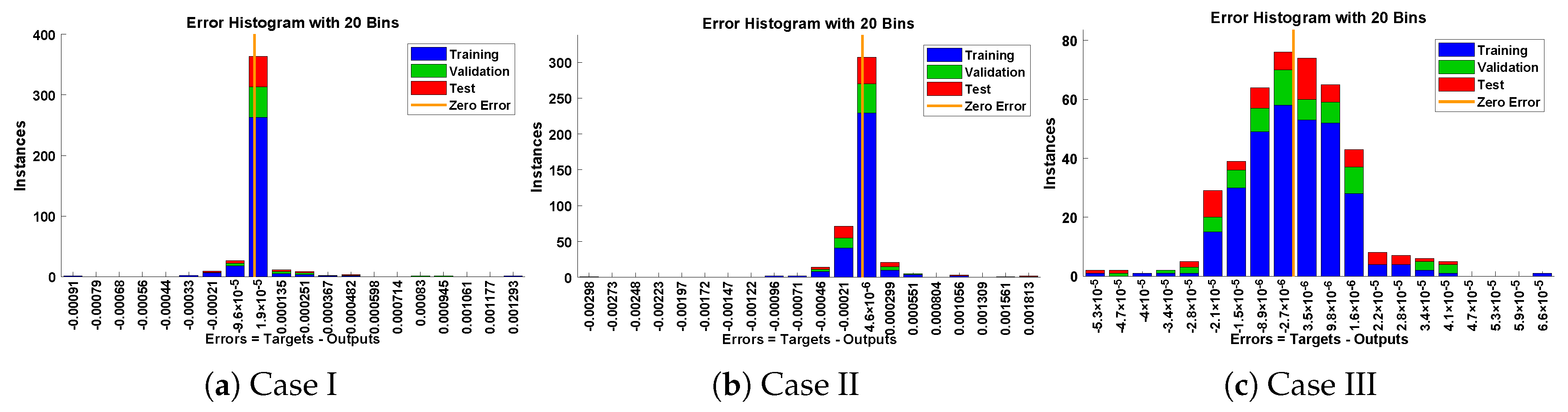
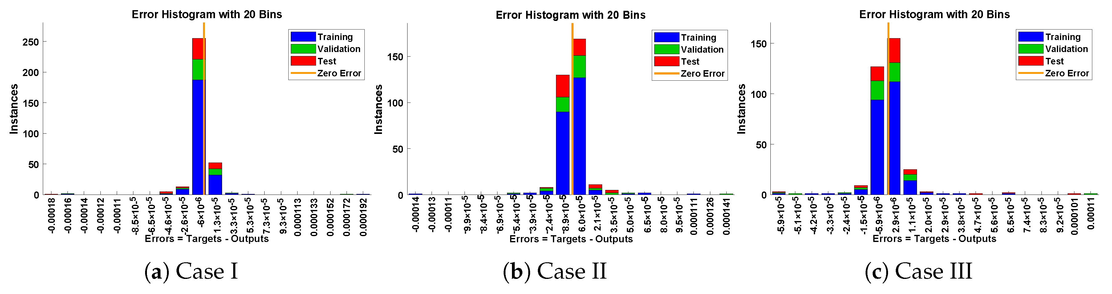
Figure 18.
Error histogram analysis for each case of restrained uniform beam carrying an intermediate lumped mass.
Figure 18.
Error histogram analysis for each case of restrained uniform beam carrying an intermediate lumped mass.
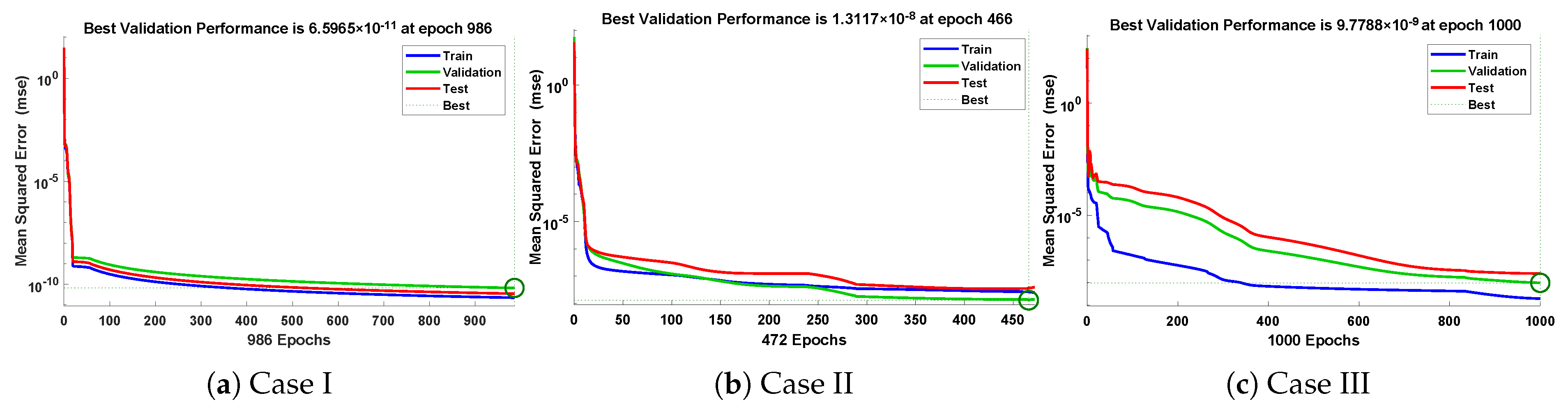
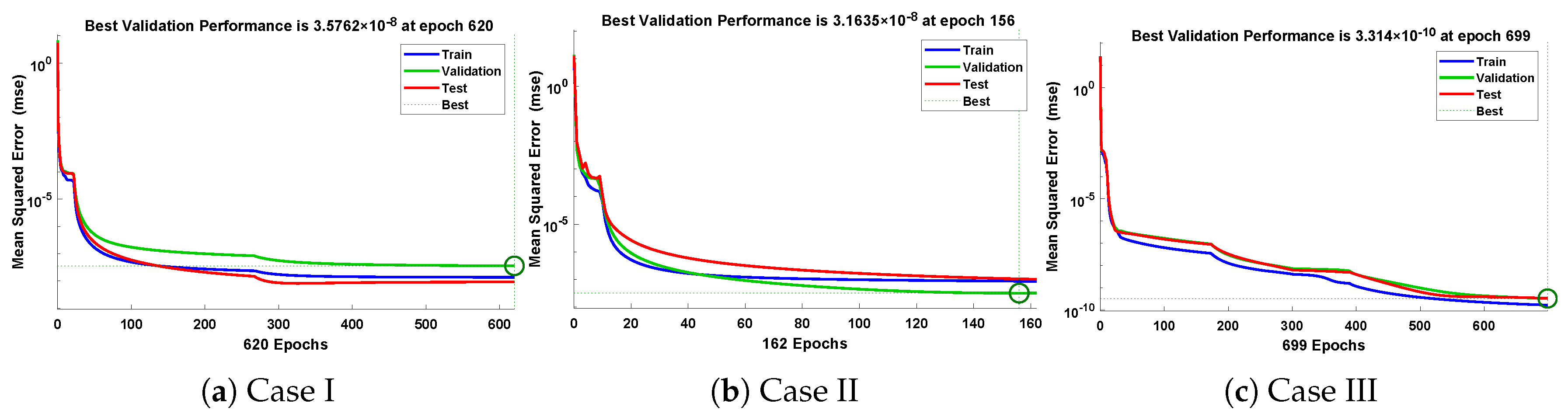
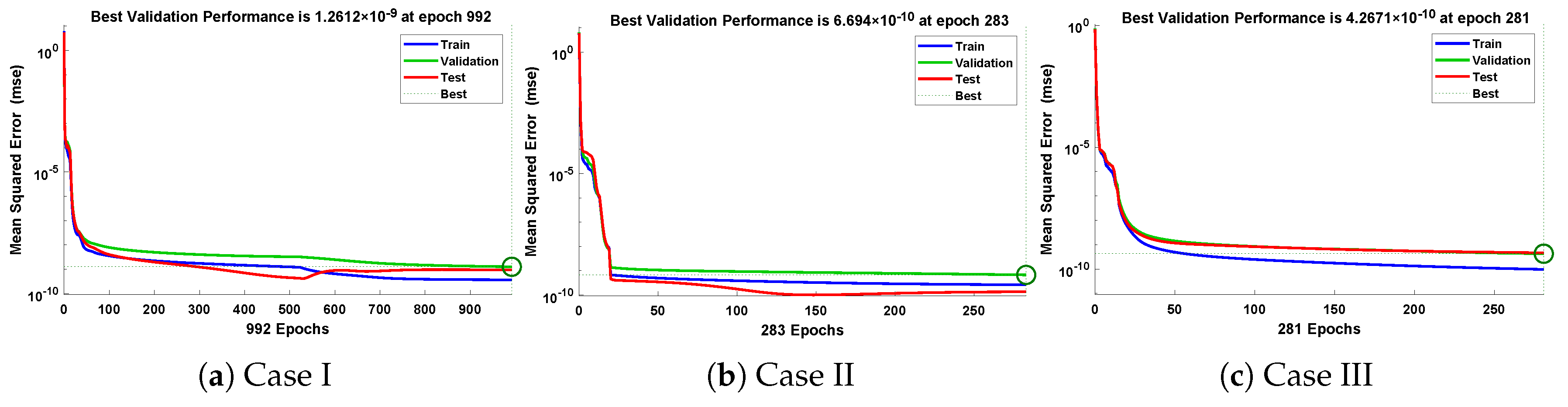
Figure 19.
Convergence of performance function in terms of mean square error for each case of problem 3.
Figure 19.
Convergence of performance function in terms of mean square error for each case of problem 3.
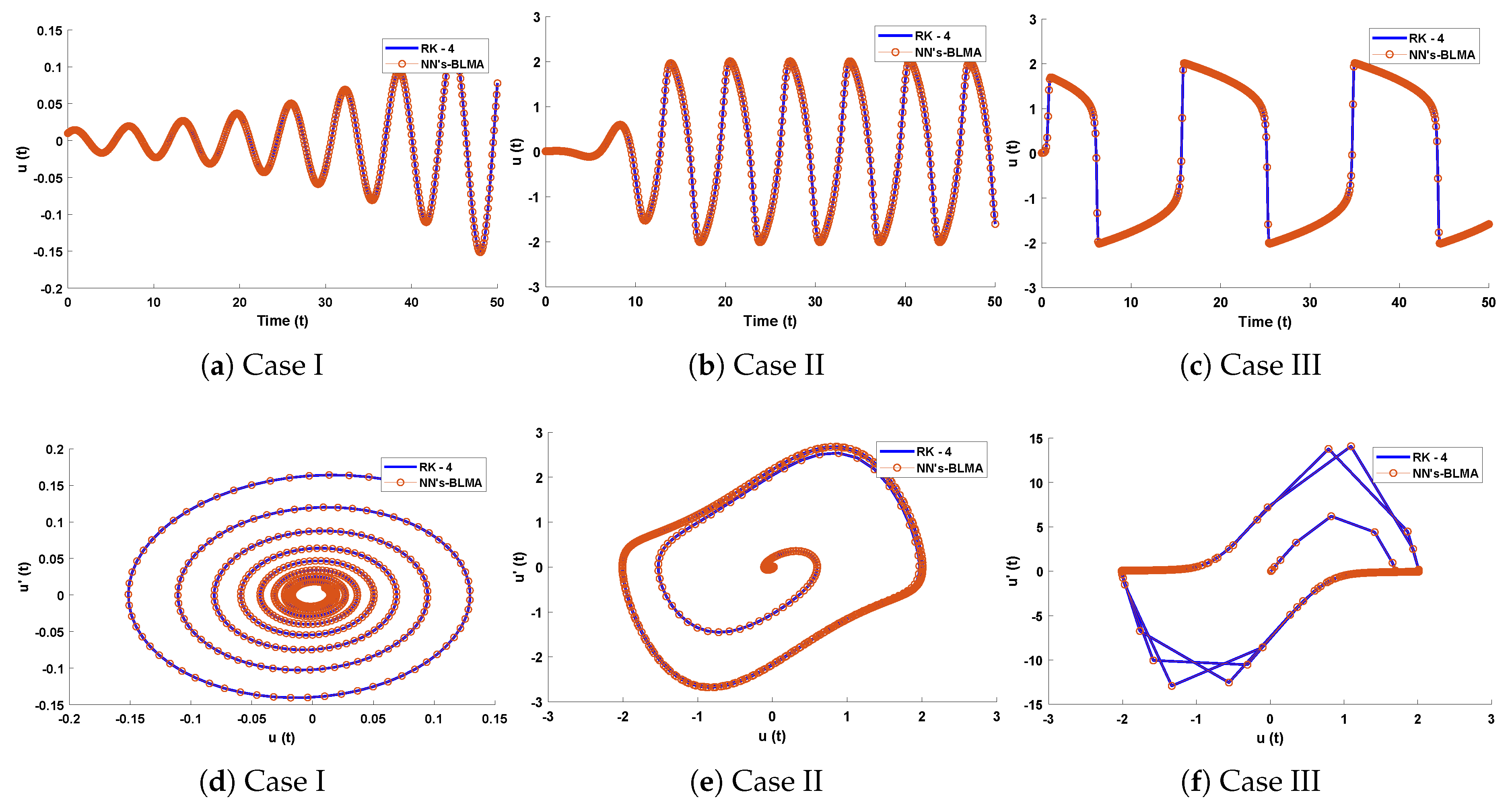
Figure 20.
(a–c) Comparison of approximate solutions obtained by designed algorithm with RK-4. (d–f) show the analysis of phase plane between velocity and acceleration for van der Pol equation.
Figure 20.
(a–c) Comparison of approximate solutions obtained by designed algorithm with RK-4. (d–f) show the analysis of phase plane between velocity and acceleration for van der Pol equation.
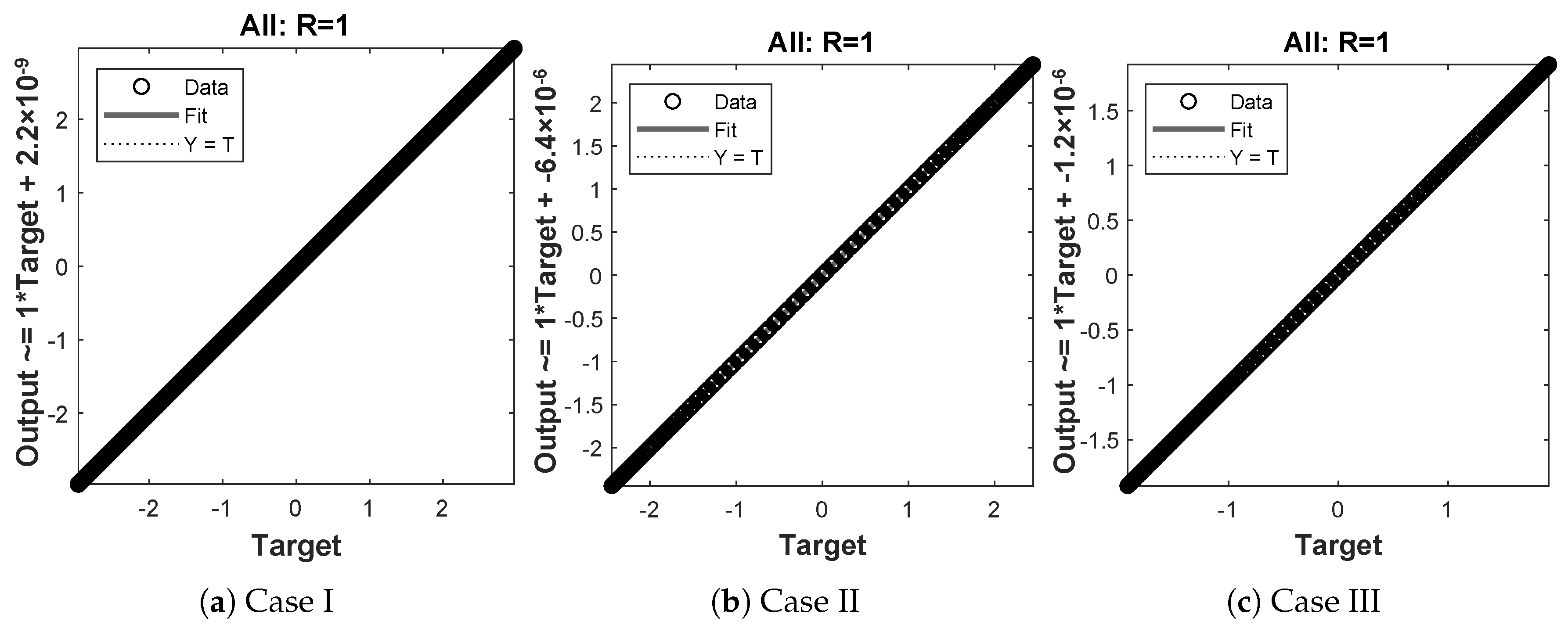
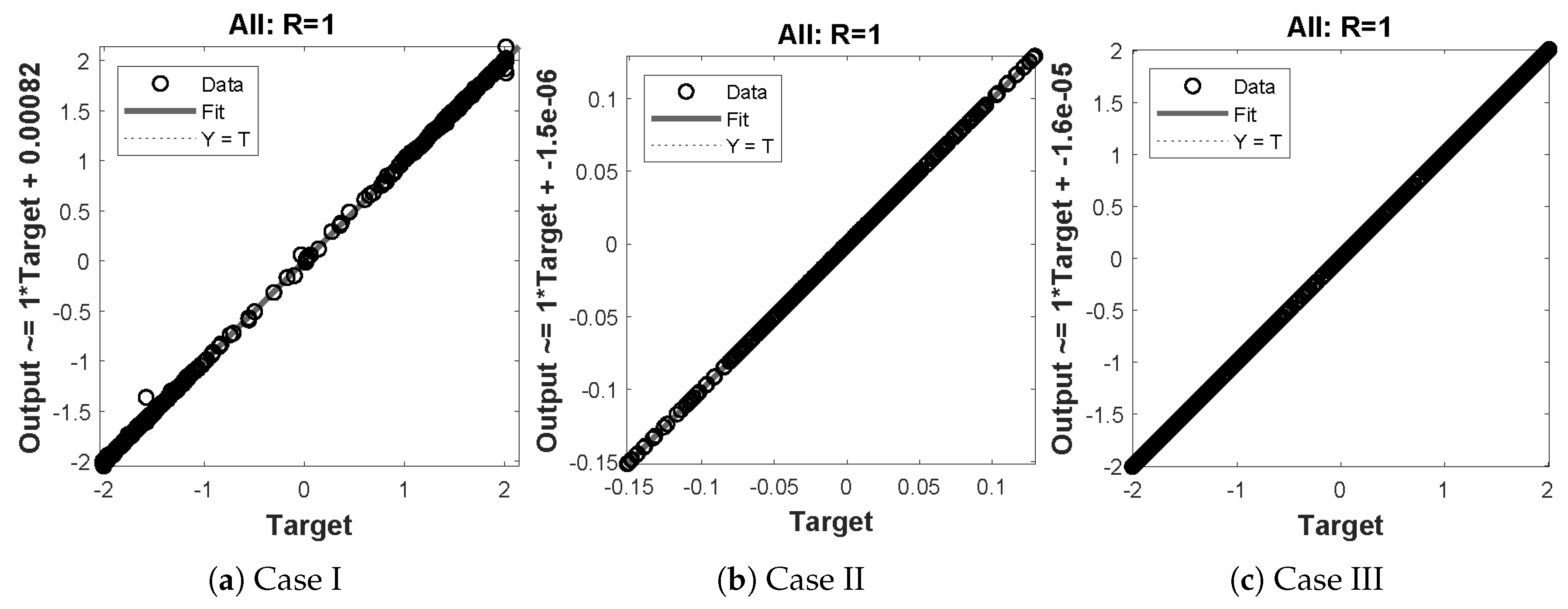
Figure 21.
Regression analysis for different cases of problem 4.
Figure 21.
Regression analysis for different cases of problem 4.
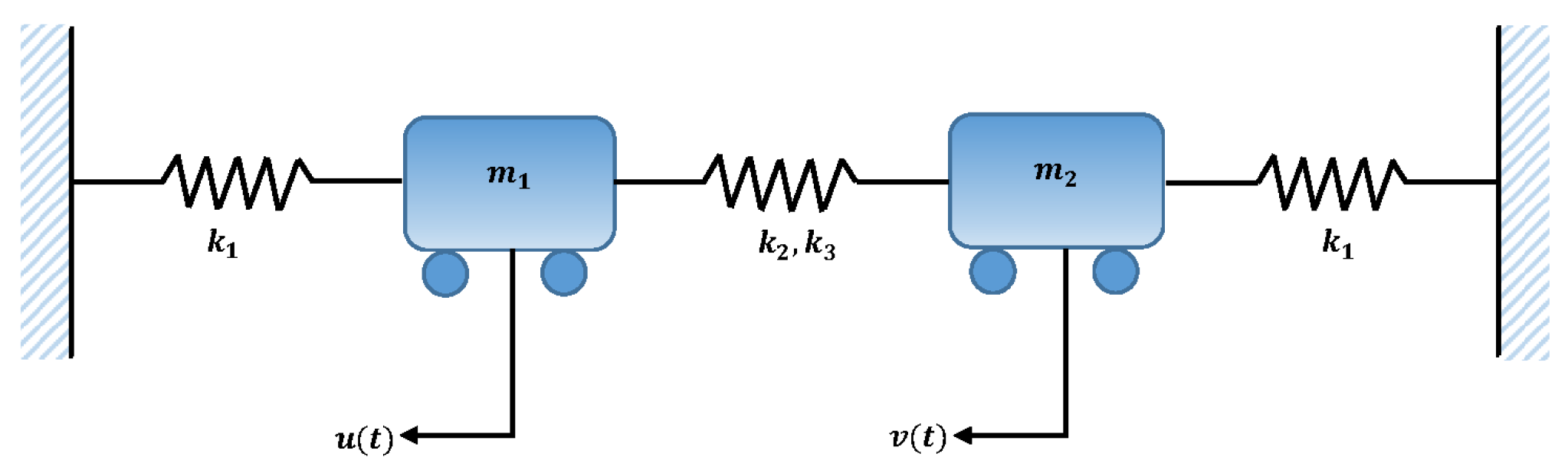
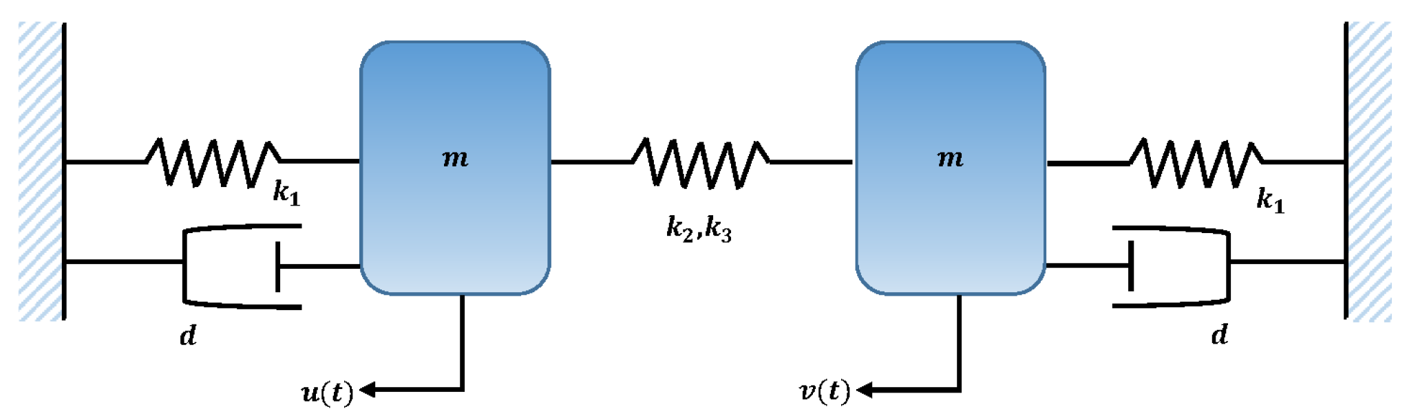
Figure 22.
Schematic of two masses attached with three springs and fixed support.
Figure 22.
Schematic of two masses attached with three springs and fixed support.
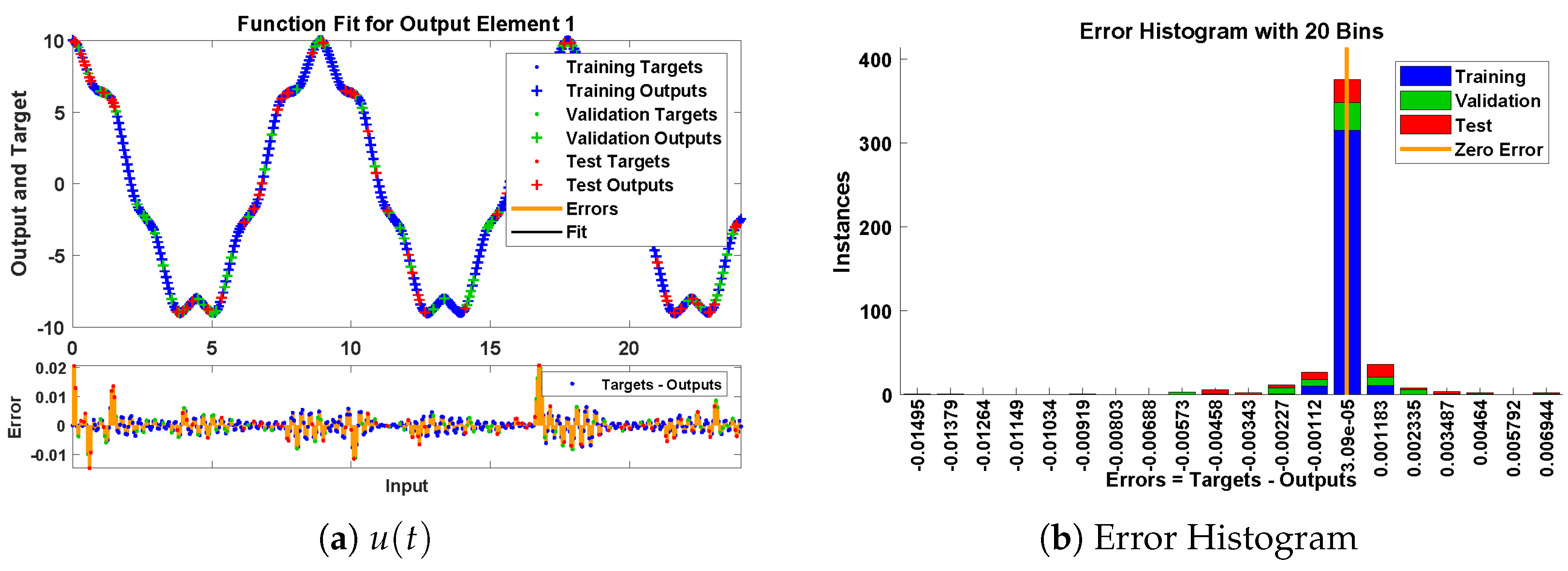
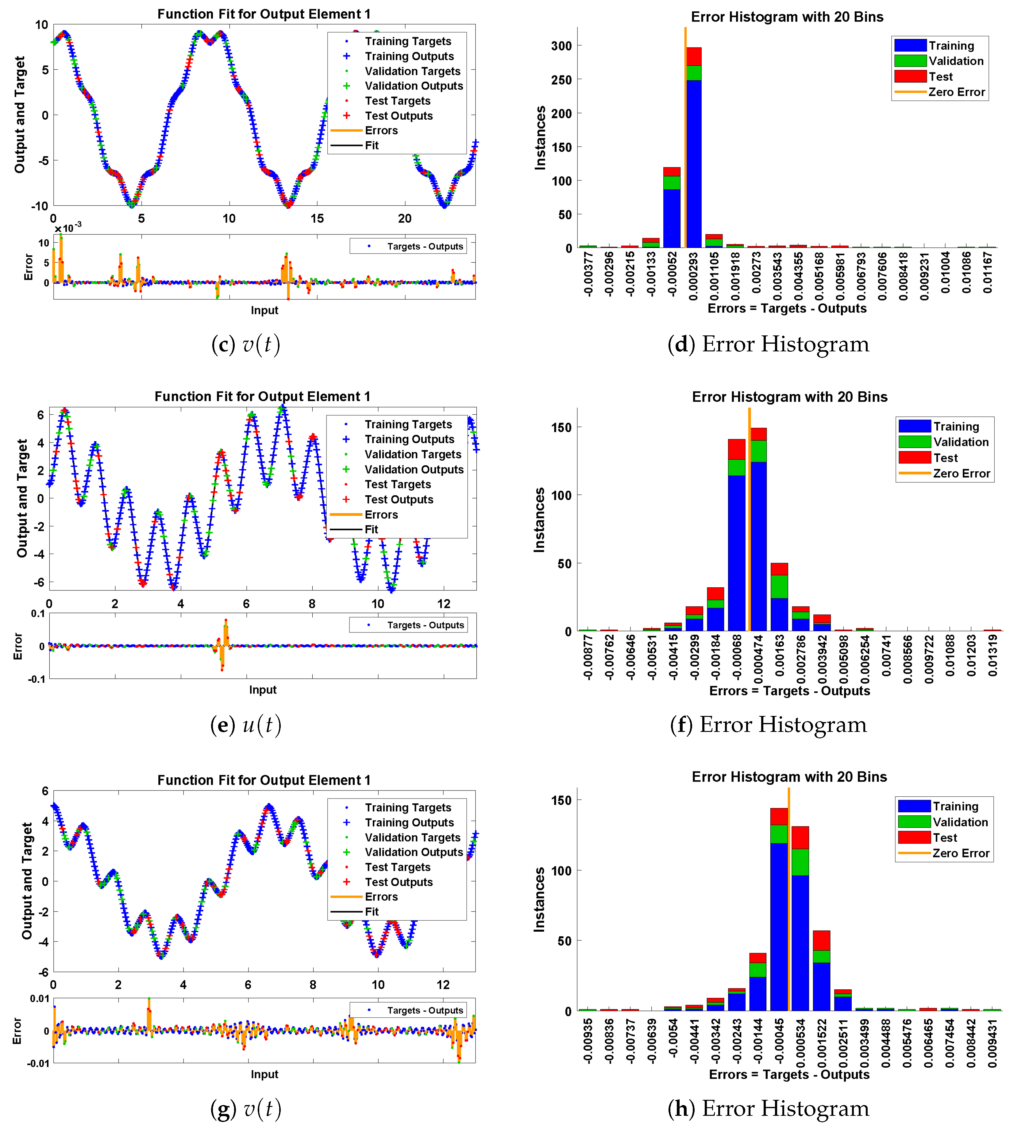
Figure 23.
Approximate solution and histograms of and for Case I and II of problem 5.
Figure 23.
Approximate solution and histograms of and for Case I and II of problem 5.
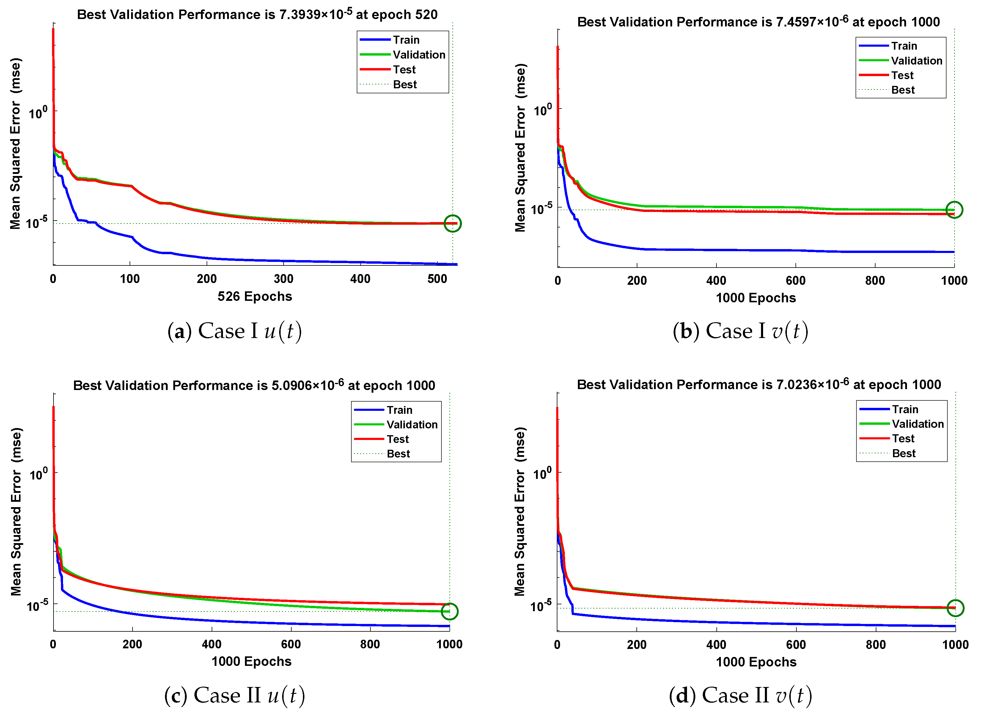
Figure 24.
Analysis of performance function in terms of mean square error for different cases of problem 5.
Figure 24.
Analysis of performance function in terms of mean square error for different cases of problem 5.
Figure 25.
Regression plots for different cases of mass attached to three springs.
Figure 25.
Regression plots for different cases of mass attached to three springs.
Figure 26.
Schematic of two masses attached with three springs and fixed support.
Figure 26.
Schematic of two masses attached with three springs and fixed support.
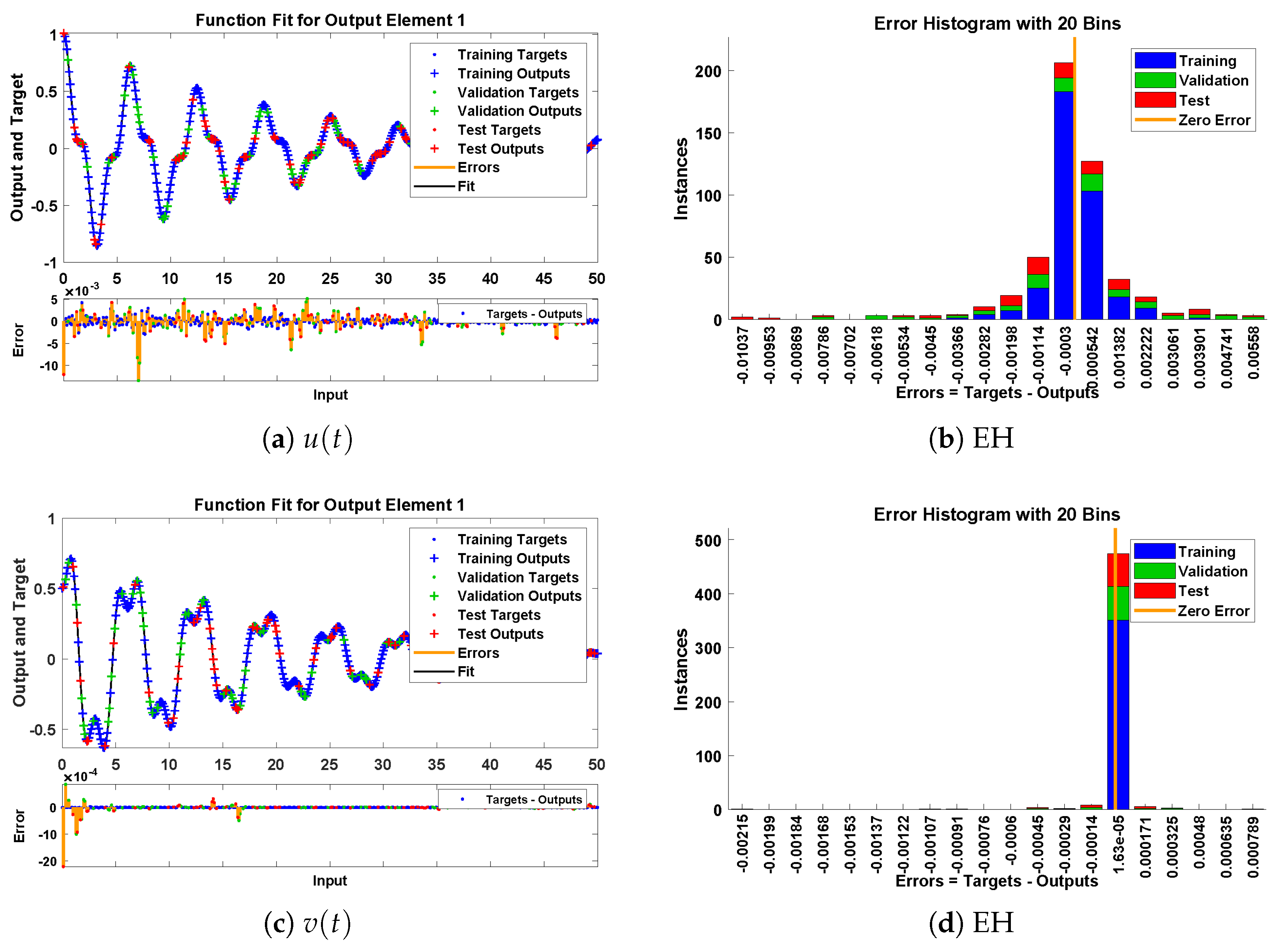
Figure 27.
Approximate solution and histograms of and for problem 6.
Figure 27.
Approximate solution and histograms of and for problem 6.
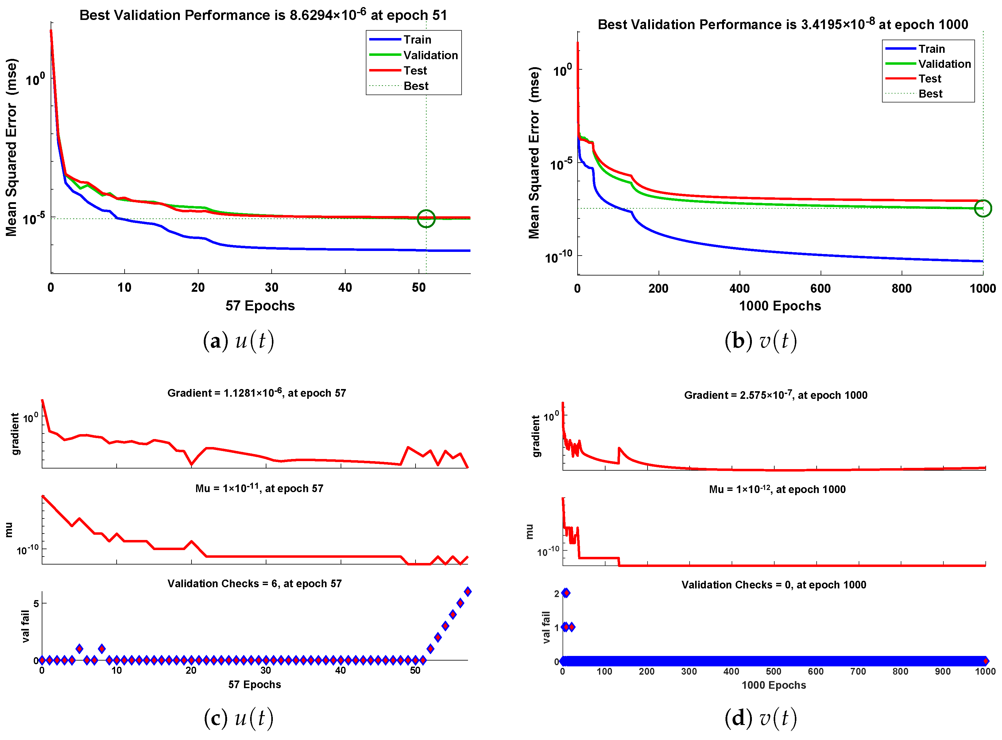
Figure 28.
Performance state of training parameters and convergence of fitness function for example 6.
Figure 28.
Performance state of training parameters and convergence of fitness function for example 6.
Table 1.
Parameter setting for the implementation of the designed NN-BLM algorithm.
Table 1.
Parameter setting for the implementation of the designed NN-BLM algorithm.
| Testing | Training | Valiation | Hidden Neurons | Max. Ilteration | Max. Validation Fails | Performance Function |
|---|
| 75% | 15% | 15% | 60 | 1000 | 6 | Mean Square Error |
Table 2.
Comparison of approximate solutions obtained by NN-BLM algorithm with He’s Energy Balance Method, Homotopy Analysis Method, Residue Harmonic Balance Method, and Homotopy Perturbation Method.
Table 2.
Comparison of approximate solutions obtained by NN-BLM algorithm with He’s Energy Balance Method, Homotopy Analysis Method, Residue Harmonic Balance Method, and Homotopy Perturbation Method.
| | Problem 1 | Problem 2 | Problem 3 | Problem 5 |
|---|
| t | Exact | HEBM | NN-BLMA | Exact | HAM | NN-BLMA | Exact | RHBM | NN-BLMA | Exact | HPM | NN-BLMA |
| 0 | 2.96706 | 3.01652 | 2.96706 | 1.5 | 1.5 | 1.5 | 1 | 1 | 1 | 8 | 7.999 | 8 |
| 3 | −2.15119 | −2.25409 | −2.15119 | −0.33557 | −0.33647 | −0.33557 | −0.99448 | −0.99442 | −0.99448 | −5.69251 | −5.69215 | −5.69251 |
| 6 | −1.13609 | −1.13986 | −1.13609 | −1.27728 | −1.218 | −1.27728 | 0.97792 | 0.97364 | 0.97792 | −5.01246 | −5.01245 | −5.01246 |
| 9 | 2.89554 | 2.99654 | 2.89554 | 0.97753 | 0.96723 | 0.97753 | −0.95033 | −0.95047 | −0.95033 | 8.10448 | 8.10448 | 8.10448 |
| 12 | −2.69881 | −2.831 | −2.69881 | 0.72292 | 0.722911 | 0.72292 | 0.91174 | 0.91177 | 0.91174 | −6.08405 | −6.08401 | −6.08405 |
| 15 | 0.12032 | 0.12087 | 0.12032 | −1.4209 | −1.42119 | −1.4209 | −0.86222 | −0.86245 | −0.86222 | −4.07551 | −4.07555 | −4.07551 |
Table 3.
Approximate solutions for angular displacements of problems 1, 2, and 3.
Table 3.
Approximate solutions for angular displacements of problems 1, 2, and 3.
| | Problem 1 | Problem 2 | Problem 3 |
|---|
| t | Case I | Case II | Case III | Case I | Case II | Case III | Case I | Case II | Case III |
| 0 | 2.96706 | 2.44346 | 1.91986 | 0.5 | 1 | 1.5 | 1 | 0.5 | 0.2 |
| 3 | −2.15119 | −2.07124 | −1.36661 | −0.49397 | −0.70011 | −0.33557 | −0.99448 | −0.47592 | −0.19447 |
| 6 | −1.13609 | 0.8869 | −0.14399 | 0.47604 | 0.00452 | −1.27728 | 0.97792 | 0.40334 | 0.17801 |
| 9 | 2.89554 | 0.71232 | 1.53846 | −0.44663 | 0.69344 | 0.97753 | −0.95033 | −0.2829 | −0.15114 |
| 12 | −2.69881 | −1.97792 | −1.90429 | 0.40645 | −0.99995 | 0.72292 | 0.91174 | 0.12156 | 0.11487 |
| 15 | 0.12032 | 2.4389 | 1.16415 | −0.35648 | 0.70671 | −1.4209 | −0.86222 | 0.06023 | −0.07096 |
Table 4.
Statistics of performance measures for obtaining solutions to problems 1 and 2.
Table 4.
Statistics of performance measures for obtaining solutions to problems 1 and 2.
| | | Mean Square Error | | | | | |
|---|
| Case | Neurons | Training | Validation | Testing | Gradient | Mu | Epochs | Regression | Time |
| I | 60 | | | | | | 985 | 1 | 2 s |
| II | 60 | | | | | | 472 | 1 | 0.01 s |
| III | 60 | | | | | | 1000 | 1 | 2 s |
| I | 60 | | | | | | 620 | 1 | 0.03 s |
| II | 60 | | | | | | 162 | 1 | 1s |
| III | 60 | | | | | | 699 | 1 | 0.02 s |
Table 5.
Values of parameters involved in mathematical model of restrained uniform beam carrying an intermediate lumped mass.
Table 5.
Values of parameters involved in mathematical model of restrained uniform beam carrying an intermediate lumped mass.
| Cases | Amplitude (A) | | | | |
|---|
| I | 1 | 0.326845 | 0.129579 | 0.232598 | 0.087584 |
| II | 0.5 | 1.642033 | 0.913055 | 0.313561 | 0.204297 |
| III | 0.2 | 4.051486 | 1.665232 | 0.281418 | 0.149677 |
Table 6.
Statistics of performance measures for obtaining solutions to problems 3 and 4.
Table 6.
Statistics of performance measures for obtaining solutions to problems 3 and 4.
| | | Mean Square Error | | | | | |
|---|
| Case | Neurons | Training | Validation | Testing | Gradient | Mu | Epochs | Regression | Time |
| I | 60 | 3.67 × 10 | 1.26 × 10 | 9.37 × 10 | 9.98 × 10 | 1.00 × 10 | 992 | 1 | 0.02 s |
| II | 60 | 2.61 × 10 | 6.69 × 10 | 1.35 × 10 | 9.97 × 10 | 1.00 × 10 | 283 | 1 | 0.01 s |
| III | 60 | 9.69 × 10 | 4.27 × 10 | 4.63 × 10 | 9.97 × 10 | 1.00 × 10 | 281 | 1 | 0.01 s |
| I | 60 | 3.76 × 10 | 2.36 × 10 | 3.16 × 10 | 9.95 × 10 | 1.00 × 10 | 100 | 1 | 0.005 s |
| II | 60 | 5.27 × 10 | 2.08 × 10 | 2.99 × 10 | 1.72 × 10 | 1.00 × 10 | 1000 | 1 | 2 s |
| III | 60 | 1.02 × 10 | 9.57 × 10 | 6.91 × 10 | 6.09 × 10 | 1.00 × 10 | 340 | 1 | 0.02 s |
Table 7.
Approximate solutions for displacement of problems 4, 5, and 6.
Table 7.
Approximate solutions for displacement of problems 4, 5, and 6.
| | Problem 4 | Problem 5 | Problem 6 |
|---|
| t | Case I | Case II | Case III | Case I | Case II | Case I |
| | | | | |
| 0 | 0.01 | 0.01 | 0.01 | 8 | 10 | 5 | 1 | 1 | 0.5 |
| 3 | −0.0099 | −0.02498 | 1.50214 | −5.69251 | −3.7239 | −3.07566 | −4.7436 | −0.84116 | −0.42692 |
| 6 | 0.00925 | −0.00824 | 0.44609 | −5.01246 | −3.13545 | 2.24812 | 4.25251 | 0.67892 | 0.36974 |
| 9 | −0.00791 | 0.42076 | −1.83206 | 8.10448 | 9.83682 | −2.90897 | 1.08233 | −0.51973 | −0.327 |
| 12 | 0.00571 | −1.03501 | −1.56265 | −6.08405 | −4.53945 | 0.00641 | 1.33001 | 0.37165 | 0.29367 |
| 15 | −0.00244 | 1.39666 | −1.03589 | −4.07551 | −2.75077 | 1.67698 | −0.64469 | −0.24233 | −0.26364 |
Table 8.
Statistics of performance measures by NN-BLMA for obtaining solutions to problems 5 and 6.
Table 8.
Statistics of performance measures by NN-BLMA for obtaining solutions to problems 5 and 6.
| | | Mean Square Error | | | | | |
|---|
| Case | Neurons | Training | Validation | Testing | Gradient | Mu | Epochs | Regression | Time |
| I | 60 | 1.03 × 10 | 7.39 × 10 | 7.68 × 10 | 2.63 × 10 | 1.00 × 10 | 526 | 1 | 0.06 s |
| 60 | 5.48 × 10 | 7.46 × 10 | 4.58 × 10 | 2.17 × 10 | 1.00 × 10 | 1000 | 1 | 2 s |
| II | 60 | 1.43 × 10 | 5.09 × 10 | 9.57 × 10 | 1.54 × 10 | 1.00 × 10 | 1000 | 1 | 2 s |
| 60 | 1.46 × 10 | 7.02 × 10 | 7.38 × 10 | 2.55 × 10 | 1.00 × 10 | 1000 | 1 | 2 s |
| I | 60 | 4.96 × 10 | 3.42 × 10 | 8.76 × 10 | 2.58 × 10 | 1.00 × 10 | 1000 | 1 | 2 s |
| 60 | 6.18 × 10 | 8.63 × 10 | 9.52 × 10 | 1.13 × 10 | 1.00 × 10 | 57 | 1 | 0.001 s |


 ,
, 


