
The Downlink Performance for Cell-Free Massive MIMO with Instantaneous CSI in Slowly Time-Varying Channels


Abstract
:1. Introduction
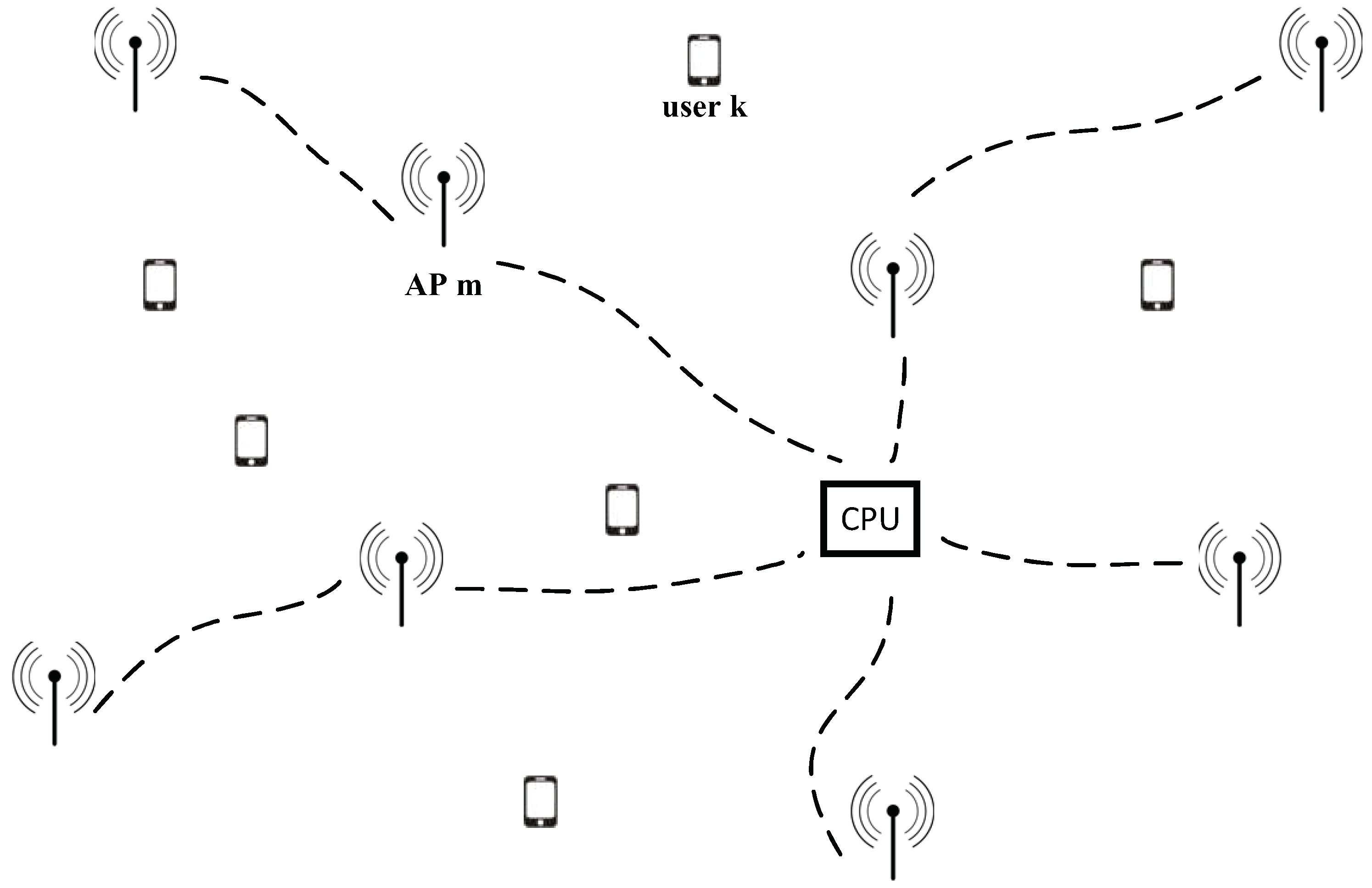
2. System Model
2.1. Channel Hardening
2.2. Favorable Propagation
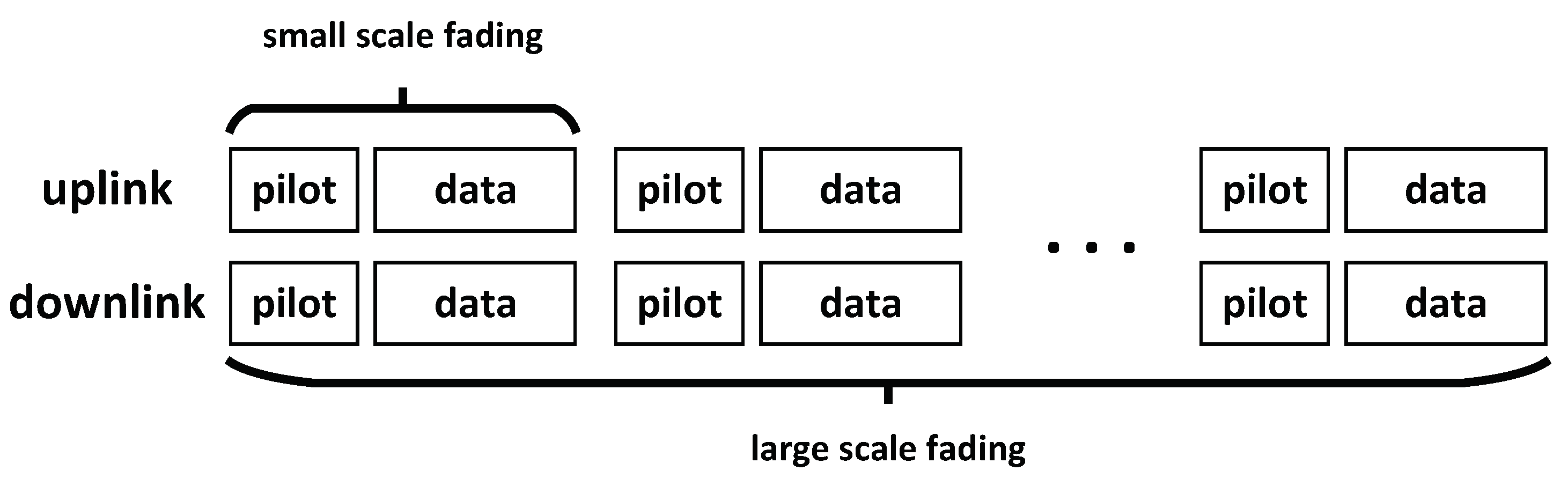
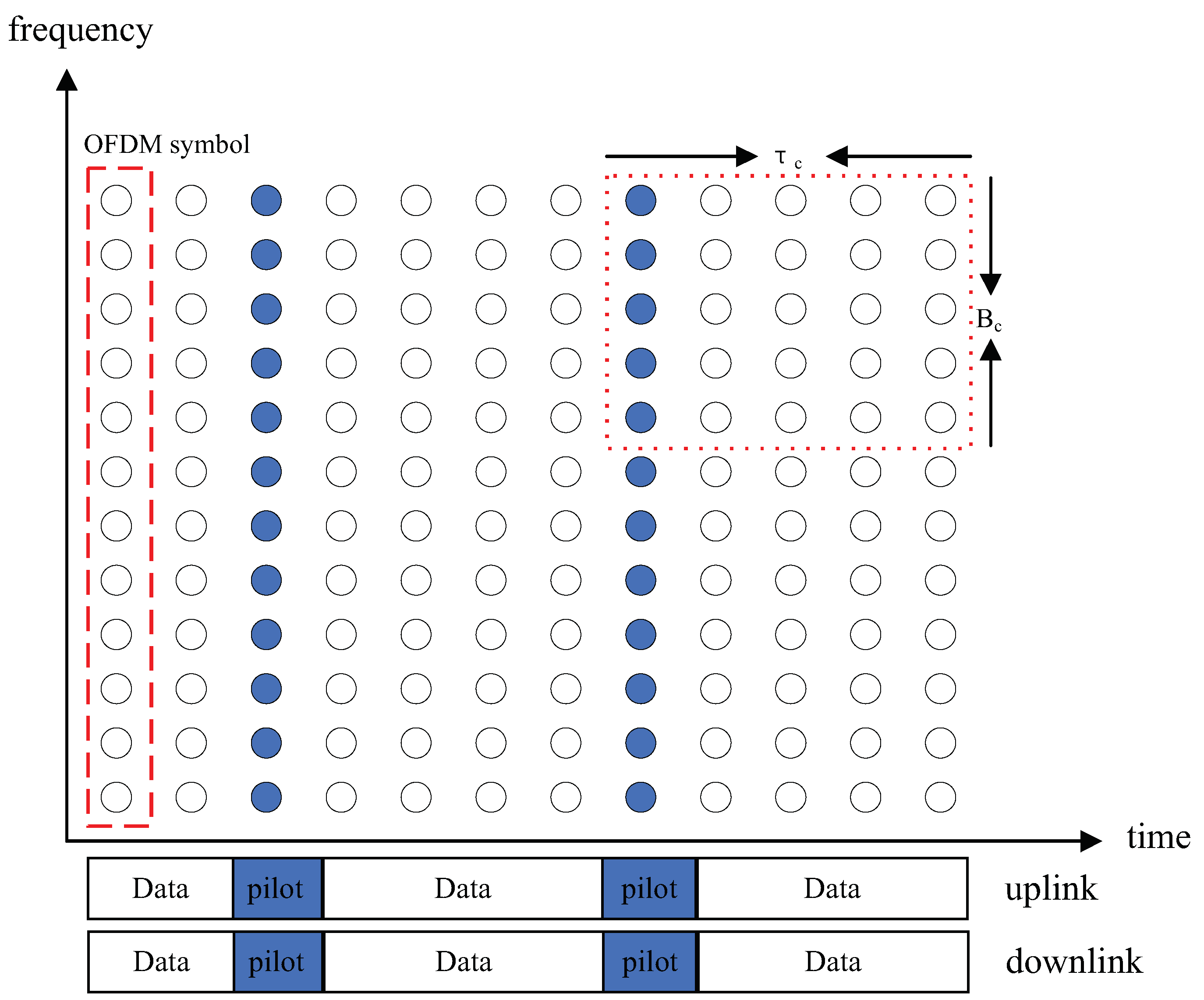
2.3. Downlink Transmission and Minimum Mean Square Error (MMSE) Estimation
3. CB and Power Control
3.1. CB with Instantaneous CSI
3.2. Power Control
4. Quantization of CSI Feedback
5. Results
5.1. Comparison of Different Schemes
5.2. Comparison of Different Numbers of Quantization Bits
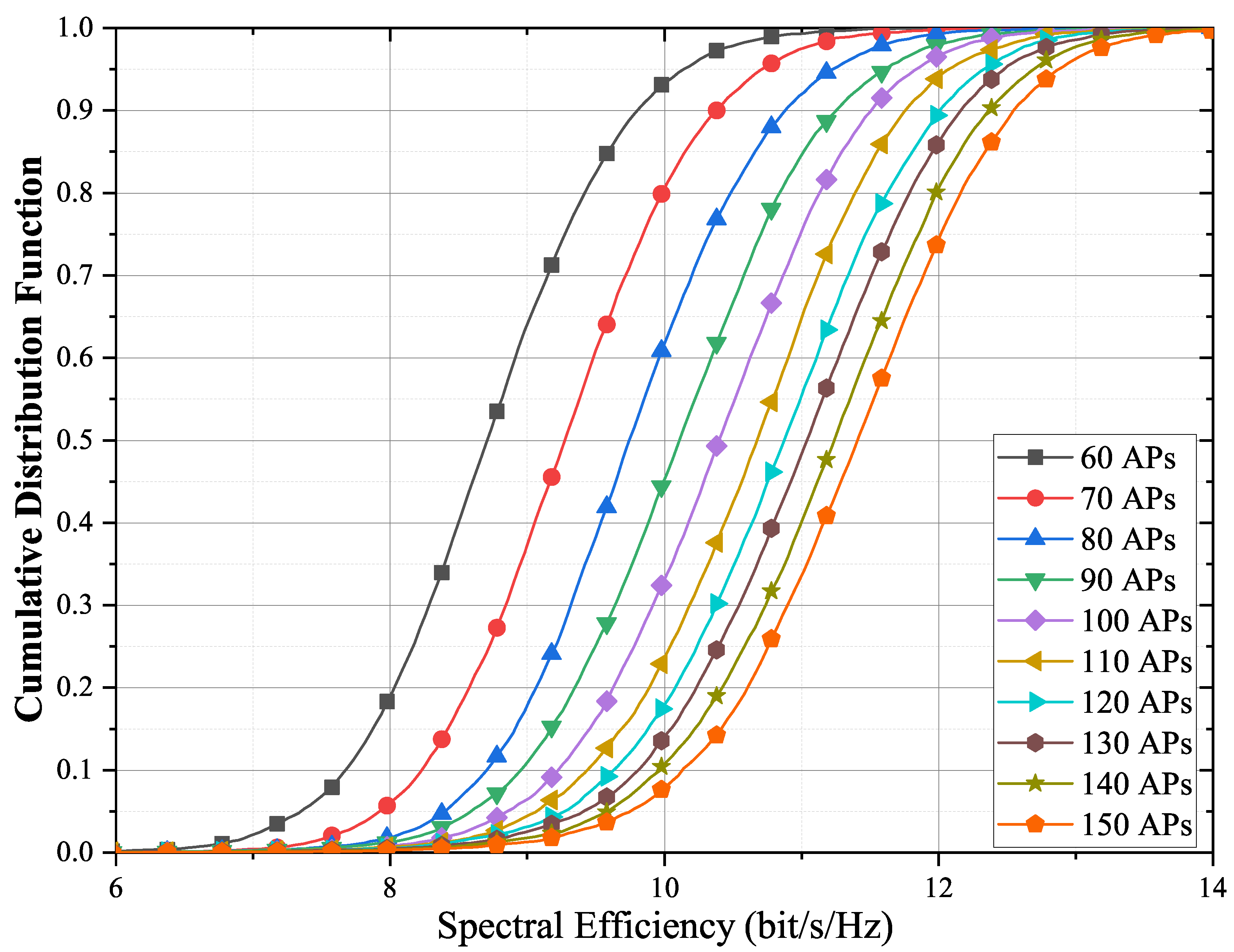
5.3. Comparison of Different Numbers of APs and UE
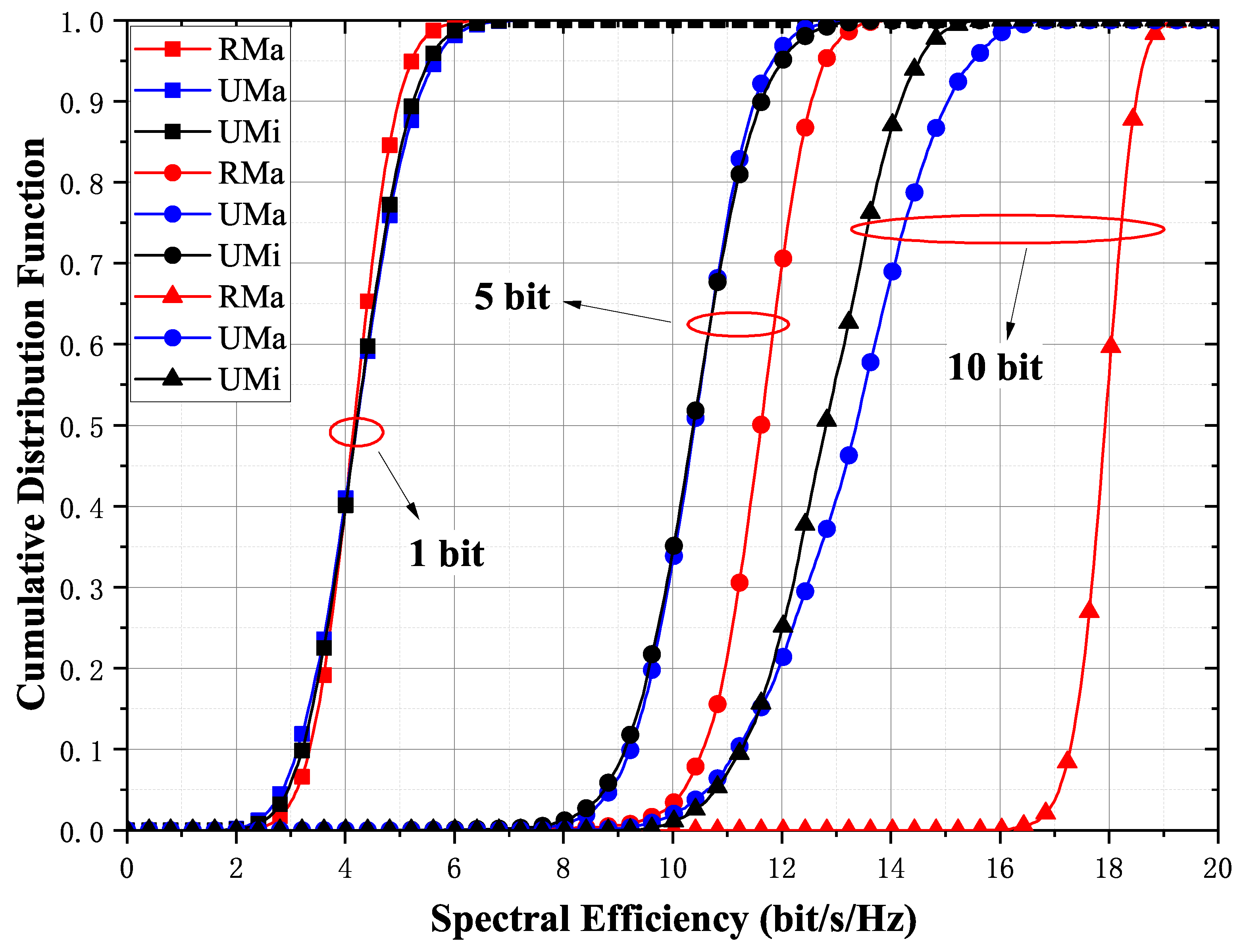
5.4. Comparison of Rural-Macro (RMa), Urban-Macro (UMa), and UMi Scenarios
6. Conclusions
Author Contributions
Funding
Conflicts of Interest
References
- Cisco. Cisco Visual Networking Index: Forecast and Trends, 2018–2022, White Paper; Cisco: San Jose, CA, USA, 2020. [Google Scholar]
- Akyildiz, I.F.; Kak, A.; Nie, S. 6G and beyond: The future of wireless communications systems. IEEE Access 2020, 8, 133995–134030. [Google Scholar] [CrossRef]
- Zhang, J.; Björnson, E.; Matthaiou, M.; Ng, D.W.K.; Yang, H.; Love, D.J. Prospective multiple antenna technologies for beyond 5G. IEEE J. Sel. Areas Commun. 2020, 38, 1637–1660. [Google Scholar] [CrossRef]
- Papazafeiropoulos, A.; Kourtessis, P.; Di Renzo, M.; Chatzinotas, S.; Senior, J.M. Performance analysis of cell-free massive MIMO systems: A stochastic geometry approach. IEEE Trans. Veh. Technol. 2020, 69, 3523–3537. [Google Scholar] [CrossRef] [Green Version]
- Zhang, X.; Wang, J.; Poor, H.V. Statistical delay and error-rate bounded QoS provisioning for mURLLC over 6G CF M-MIMO mobile networks in the finite blocklength regime. IEEE J. Sel. Areas Commun. 2020, 39, 652–667. [Google Scholar] [CrossRef]
- Tan, F.; Wu, P.; Wu, Y.; Xia, M. Energy-efficient non-orthogonal multicast and unicast transmission of cell-free massive MIMO systems with SWIPT. IEEE J. Sel. Areas Commun. 2020, 39, 949–968. [Google Scholar] [CrossRef]
- Interdonato, G.; Björnson, E.; Quoc Ngo, H.; Frenger, P.; Larsson, E.G. Ubiquitous cell-free Massive MIMO communications. J. Wirel. Commun. Netw. 2019, 2019, 197. [Google Scholar] [CrossRef] [Green Version]
- Ngo, H.Q.; Ashikhmin, A.; Yang, H.; Larsson, E.G.; Marzetta, T.L. Cell-free massive MIMO versus small cells. IEEE Trans. Wirel. Commun. 2017, 16, 1834–1850. [Google Scholar] [CrossRef] [Green Version]
- Liu, P.; Luo, K.; Chen, D.; Jiang, T. Spectral efficiency analysis of cell-free massive MIMO systems with zero-forcing detector. IEEE Trans. Wirel. Commun. 2020, 19, 795–807. [Google Scholar] [CrossRef] [Green Version]
- Özdogan, Ö.; Bjöornson, E.; Zhang, J. Cell-free massive MIMO with Rician fading: Estimation schemes and spectral efficiency. In Proceedings of the 2018 52nd Asilomar Conference on Signals, Systems, and Computers, Pacific Grove, CA, USA, 28–31 October 2018; pp. 975–979. [Google Scholar] [CrossRef]
- Marzetta, T.L.; Larsson, E.G.; Yang, H.; Ngo, H.Q. Fundamentals of Massive MIMO; Cambridge University Press: Cambridge, UK, 2016. [Google Scholar]
- Xie, H.; Gao, F.; Jin, S.; Fang, J.; Liang, Y.-C. Channel estimation for TDD/FDD massive MIMO systems with channel covariance computing. IEEE Trans. Wirel. Commun. 2018, 17, 4206–4218. [Google Scholar] [CrossRef] [Green Version]
- Ngo, H.Q.; Ashikhmin, A.; Yang, H.; Larsson, E.G.; Marzetta, T.L. Cell-free massive MIMO: Uniformly great service for everyone. In Proceedings of the 2015 IEEE 16th International Workshop on Signal Processing Advances in Wireless Communications (SPAWC), Stockholm, Sweden, 28 June–1 July 2015; pp. 201–205. [Google Scholar] [CrossRef] [Green Version]
- Interdonato, G.; Karlsson, M.; Bjornson, E.; Larsson, E.G. Downlink spectral efficiency of cell-free massive MIMO with full-pilot zero-forcing. In Proceedings of the 2018 IEEE Global Conf. Signal and Information Processing (GlobalSIP), Anaheim, CA, USA, 26–29 November 2018; pp. 1003–1007. [Google Scholar] [CrossRef] [Green Version]
- Zheng, J.; Zhang, J.; Bjornson, E.; Ai, B. Impact of channel aging on cell-free massive MIMO over spatially correlated channels. IEEE Trans. Wirel. Commun. 2021, 20, 6451–6466. [Google Scholar] [CrossRef]
- Chen, Z.; Bjornson, E. Channel hardening and favorable propagation in cell-free massive MIMO with stochastic geometry. IEEE Trans. Commun. 2018, 66, 5205–5219. [Google Scholar] [CrossRef] [Green Version]
- Shen, J.; Zhang, J.; Alsusa, E.; Letaief, K.B. Compressed CSI acquisition in FDD massive MIMO: How much training is needed? IEEE Trans. Wirel. Commun. 2016, 15, 4145–4156. [Google Scholar] [CrossRef]
- Abdallah, A.; Mansour, M.M. Angle-based multipath estimation and beamforming for FDD cell-free massive MIMO. In Proceedings of the 2019 IEEE 20th International Workshop on Signal Processing Advances in Wireless Communications (SPAWC), Cannes, France, 2–5 July 2019; pp. 1–5. [Google Scholar] [CrossRef]
- Agrawal, D.P.; Zeng, Q.A. Introduction to Wireless and Mobile Systems; Cengage Learning: Boston, MA, USA, 2015. [Google Scholar]
- Gao, Z.; Dai, L.; Wang, Z.; Chen, S. Spatially common sparsity based adaptive channel estimation and feedback for FDD massive MIMO. IEEE Trans. Signal Process. 2015, 63, 6169–6183. [Google Scholar] [CrossRef] [Green Version]
- Cho, Y.S.; Kim, J.; Yang, W.Y.; Kang, C.G. MIMO-OFDM Wireless Communications with MATLAB; John Wiley & Sons: Weinheim, Germany, 2010. [Google Scholar]
- Narasimhan, T.L.; Chockalingam, A. Channel Hardening-Exploiting Message Passing (CHEMP) Receiver in Large-Scale MIMO Systems. IEEE J. Sel. Top. Signal Process. 2014, 8, 847–860. [Google Scholar] [CrossRef] [Green Version]
- Hochwald, B.M.; Marzetta, T.L.; Tarokh, V. Multiple-antenna channel hardening and its implications for rate feedback and scheduling. IEEE Trans. Inf. Theory 2004, 50, 1893–1909. [Google Scholar] [CrossRef]
- Polegre, A.A.; Riera-Palou, F.; Femenias, G.; Armada, A.G. New insights on channel hardening in cell-free massive MIMO networks. In Proceedings of the 2020 IEEE International Conference Communications Workshops (ICC Workshops), Dublin, Ireland, 7–11 June 2020; pp. 1–7. [Google Scholar] [CrossRef]
- Boyd, S.; Vandenberghe, L. Convex Optimization; Cambridge University Press: Cambridge, UK, 2004. [Google Scholar]
- Mezghani, A.; Nossek, J.A. Capacity lower bound of MIMO channels with output quantization and correlated noise. In Proceedings of the 2012 IEEE International Symposium Information Theory (ISIT), Cambridge, UK, 1–6 July 2012; pp. 1–5. [Google Scholar]
- 3GPP. Study on channel model for frequencies from 0.5 to 100 GHz. In 3rd Generation Partnership Project (3GPP); Report TR 38.901; 3GPP: Sophia, France, 2018. [Google Scholar]


| Massive MIMO | 0.1005 | 0.0099 | 0.001 | 9.9 | 9.98 |
| Cell-Free | 0.6173 | 0.5152 | 0.3745 | 0.1839 | 0.048 |
| Massive MIMO | 0.1001 | 0.0101 | 9.99 | 9.92 | 1.009 |
| Cell-Free | 0.1016 | 0.0107 | 0.0012 | 3.385 | 6.371 |
| Parameter | Value |
|---|---|
| Transmit Power of APs and Terminals | 200 mW |
| System Bandwidth B | 20 MHz |
| Centering Frequency | 2.0 GHz |
| Height of AP and UE Antenna | 15 m & 1.65 m |
| Noise Figure (NF) | 9 dB |
| J/K | |
| 290 K |
Publisher’s Note: MDPI stays neutral with regard to jurisdictional claims in published maps and institutional affiliations. |
© 2021 by the authors. Licensee MDPI, Basel, Switzerland. This article is an open access article distributed under the terms and conditions of the Creative Commons Attribution (CC BY) license (https://creativecommons.org/licenses/by/4.0/).
Share and Cite
Han, T.; Zhao, D. The Downlink Performance for Cell-Free Massive MIMO with Instantaneous CSI in Slowly Time-Varying Channels. Entropy 2021, 23, 1552. https://doi.org/10.3390/e23111552
Han T, Zhao D. The Downlink Performance for Cell-Free Massive MIMO with Instantaneous CSI in Slowly Time-Varying Channels. Entropy. 2021; 23(11):1552. https://doi.org/10.3390/e23111552
Chicago/Turabian StyleHan, Tongzhou, and Danfeng Zhao. 2021. "The Downlink Performance for Cell-Free Massive MIMO with Instantaneous CSI in Slowly Time-Varying Channels" Entropy 23, no. 11: 1552. https://doi.org/10.3390/e23111552
APA StyleHan, T., & Zhao, D. (2021). The Downlink Performance for Cell-Free Massive MIMO with Instantaneous CSI in Slowly Time-Varying Channels. Entropy, 23(11), 1552. https://doi.org/10.3390/e23111552