
Quantum Representations and Scaling Up Algorithms of Adaptive Sampled-Data in Log-Polar Coordinates


Abstract
:1. Introduction
2. Preliminaries
3. Quantum Data Representations and Preparation Based on Adaptive Sampling Method
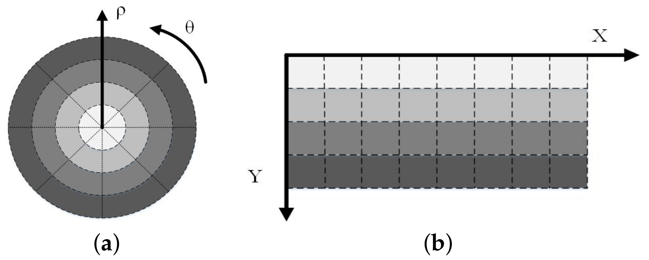
3.1. Quantum Data Representations Based on Adaptive Sampling Method
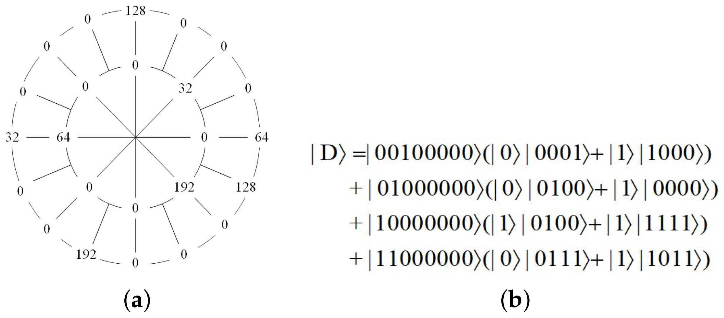
- Representing the data information as in the FRQI model
- 2.
- Representing the data information as in the NEQR model
- 3.
- Representing the data information as in the QR2-DD model
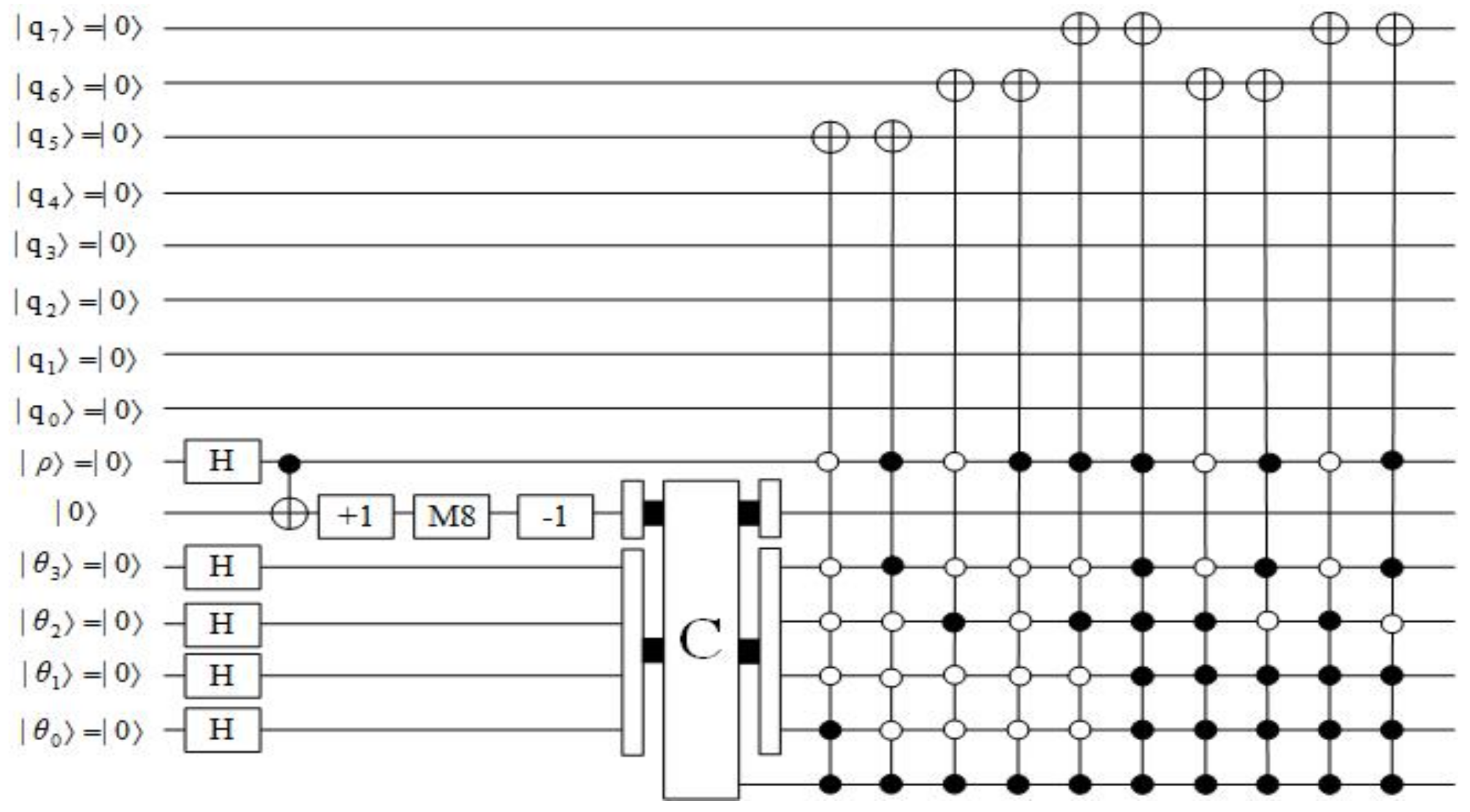
3.2. Quantum Data Preparation Based on Adaptive Sampling Method
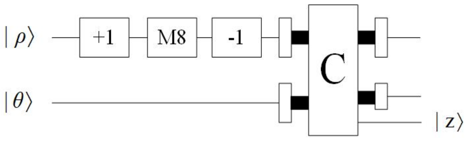
- Plus one and minus one modules
- 2.
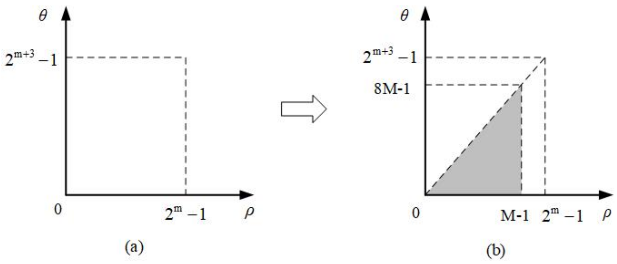
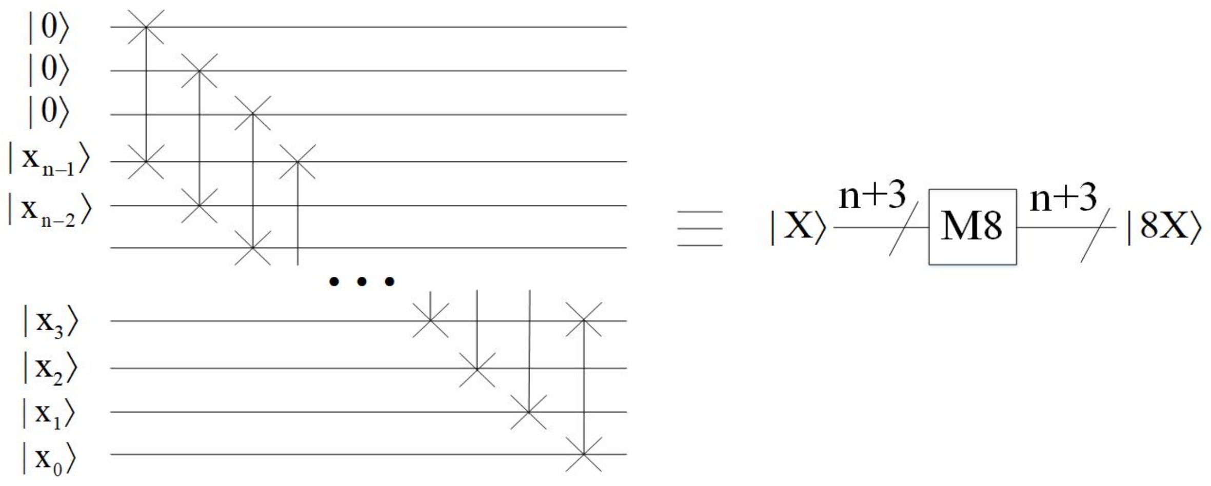
- Multiply by eight module
- 3.
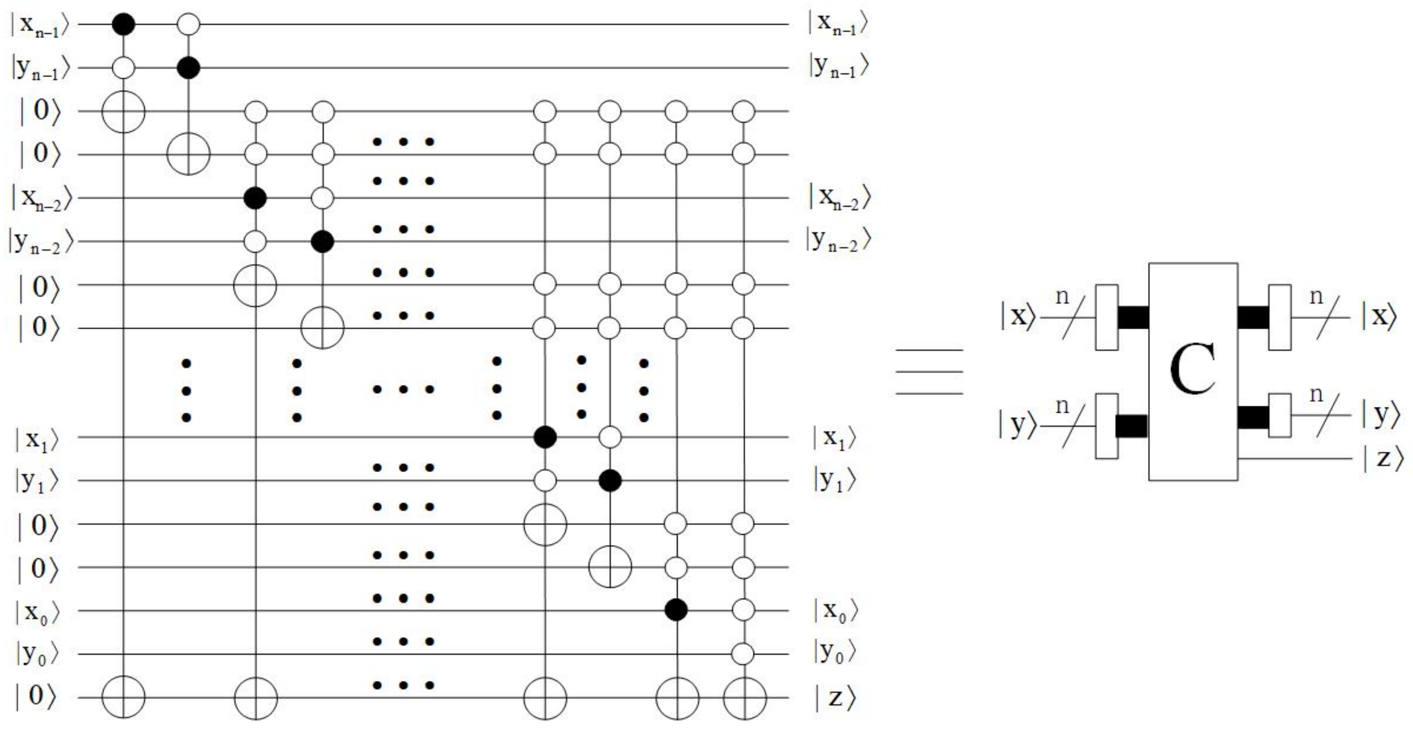
- Comparator module
3.3. Time Complexity Analysis of the Preparation Procedure
4. Quantum Data Scaling Up Algorithm with Integer Scaling Ratio Based on Biarcuate Interpolation
4.1. Quantum Circuit Modules for Arithmetic Operations
4.1.1. Multiply C- Operation Module
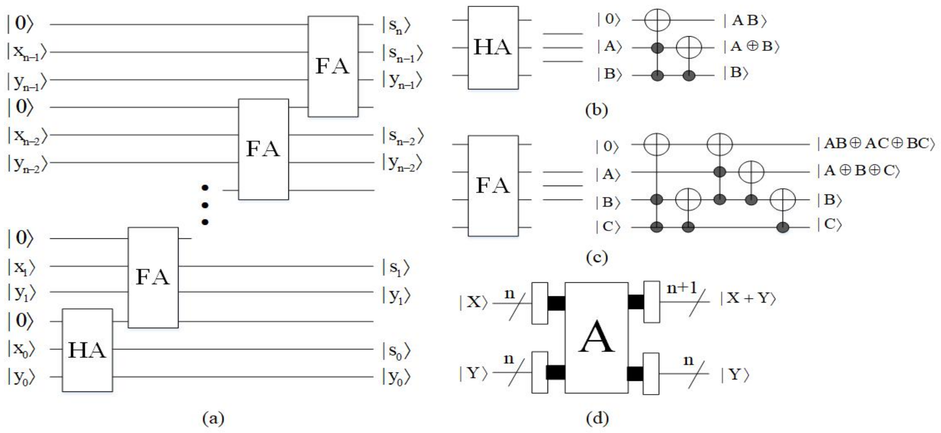
4.1.2. Adder Module
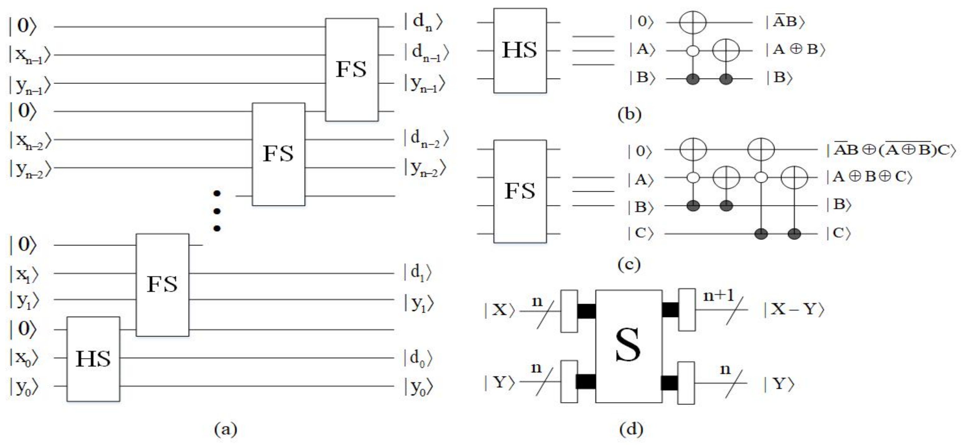
4.1.3. Subtractor Module
4.1.4. Multiplier Module
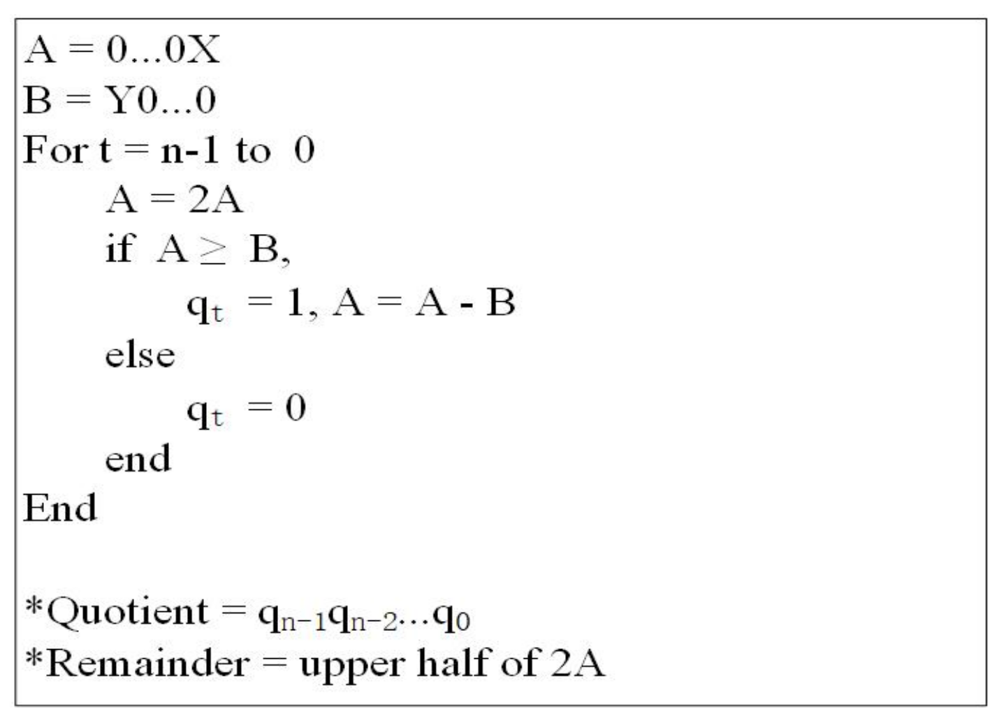
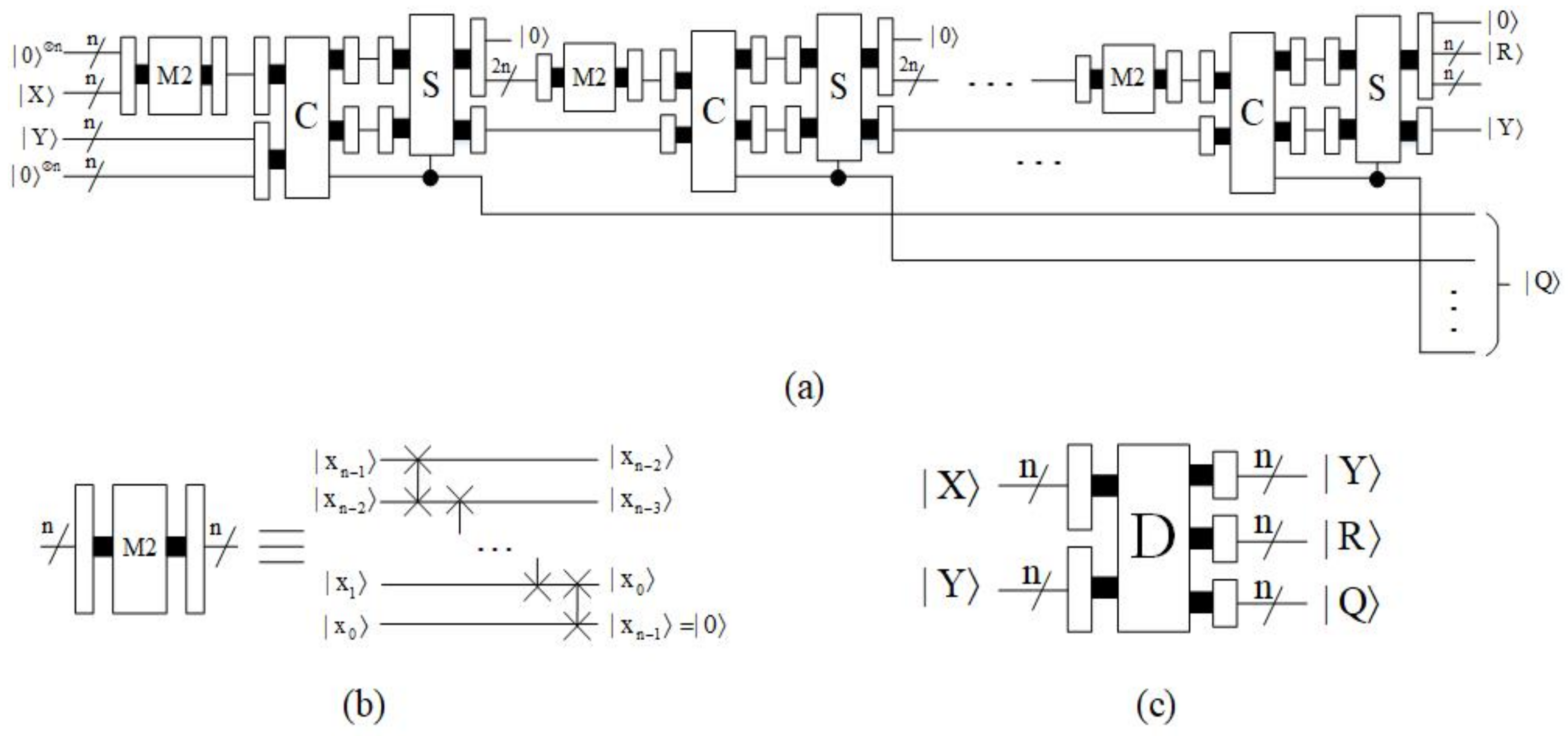
4.1.5. Divider Module
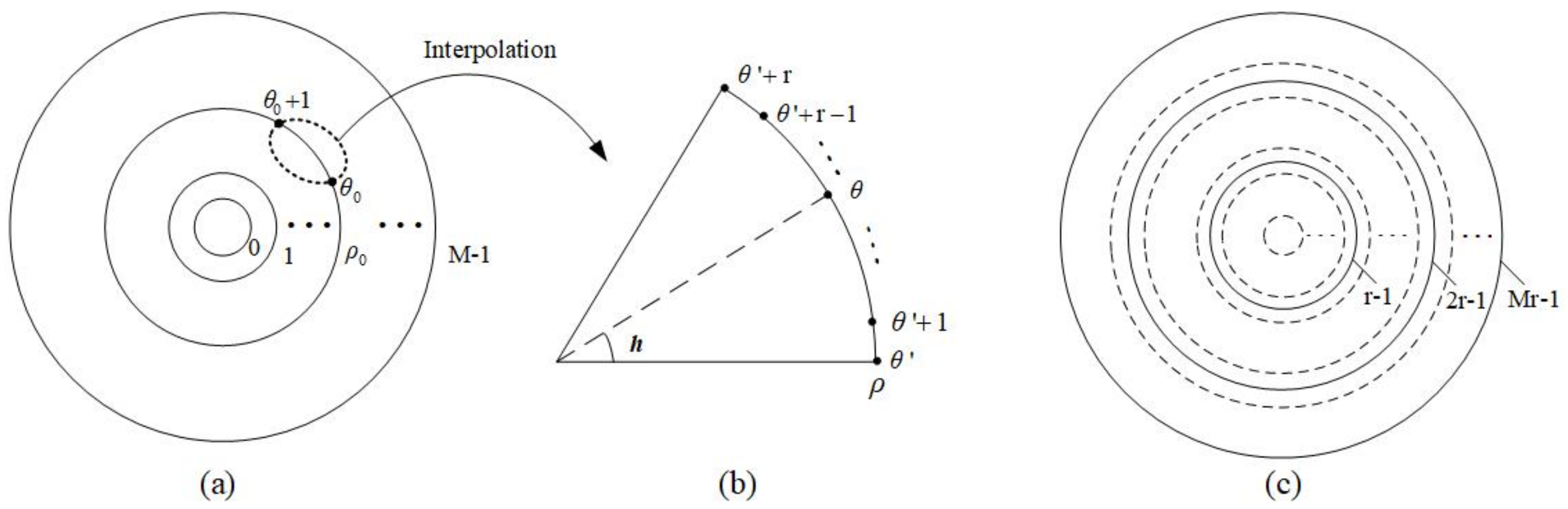
4.2. Quantum Biarcuate Interpolation Method in Log-Polar Coordinates
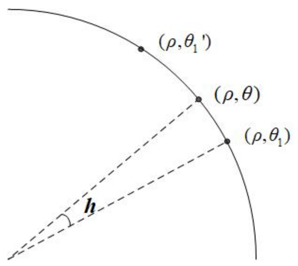
4.2.1. Arcuate Interpolation Method
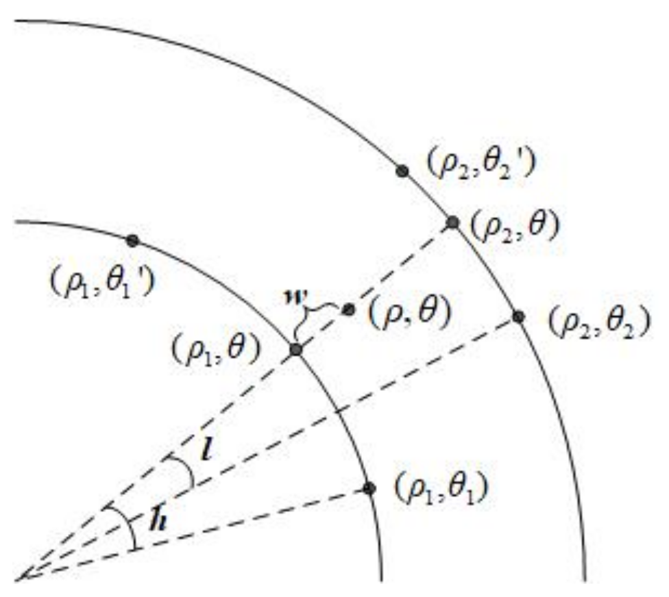
4.2.2. Biarcuate Interpolation Method
4.2.3. Quantum Realization of Biarcuate Interpolation Method
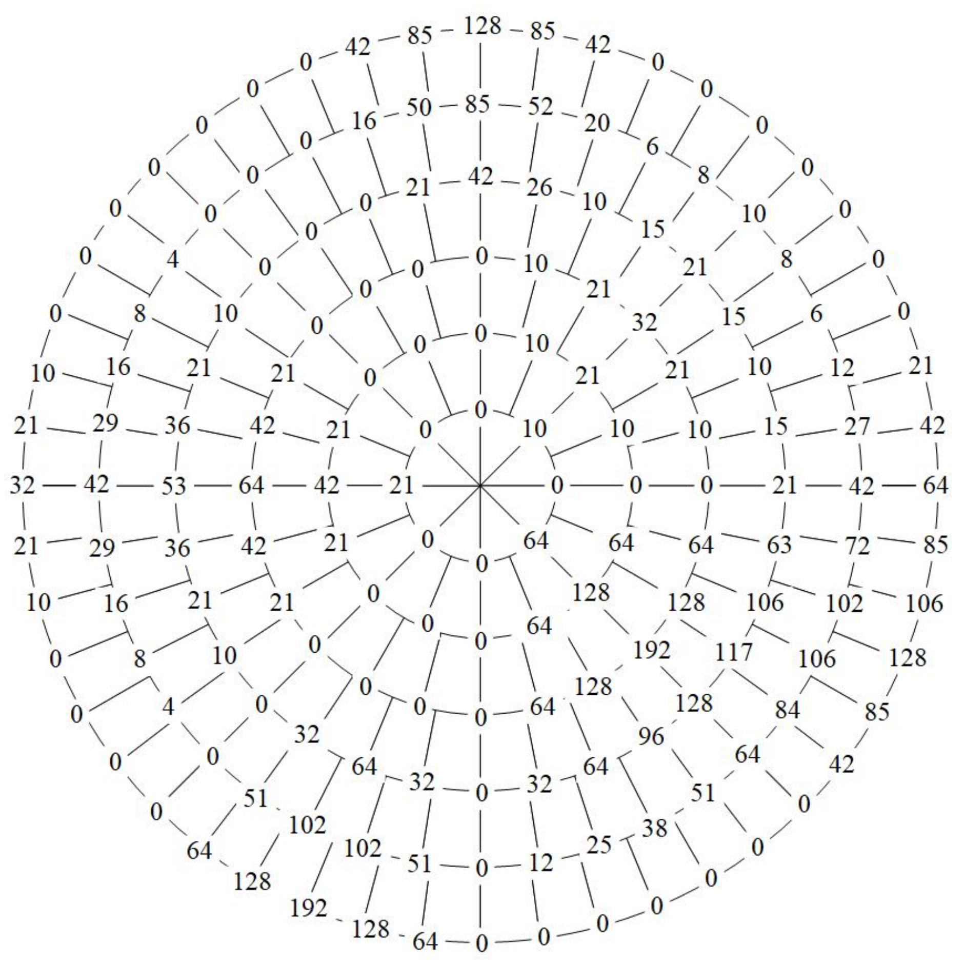
4.3. Example Verification
5. Conclusions
Author Contributions
Funding
Institutional Review Board Statement
Informed Consent Statement
Conflicts of Interest
References
- Feynman, R.P. Simulating physics with computers. Int. J. Theor. Phys 1982, 21, 467–488. [Google Scholar] [CrossRef]
- Shor, P.W. Algorithms for quantum computation: Discrete logarithms and factoring. In Proceedings of the 35th Annual Symposium on Foundations of Computer Science, Santa Fe, NM, USA, 20–22 November 1994; pp. 124–134. [Google Scholar]
- Grover, L.K. A fast quantum mechanical algorithm for database search. In Proceedings of the 28th Annual ACM Symposium on the Theory of Computing (STOC), Philadelphia, PA, USA, 22–24 May 1996; pp. 212–219. [Google Scholar]
- Venegas-Andraca, S.E.; Bose, S. Storing, processing and retrieving an image using quantum mechanics. In Proceedings of the SPIE 5105, Quantum Information and Computation, Orlando, FL, USA, 21–25 April 2003; pp. 137–147. [Google Scholar]
- Latorre, J.I. Image compression and entanglement. arXiv 2005, arXiv:quant-ph/0510031. [Google Scholar]
- Venegas-Andraca, S.E.; Ball, J.L. Processing images in entangled quantum systems. Quantum Inf. Process. 2010, 9, 1–11. [Google Scholar] [CrossRef]
- Le, P.Q.; Dong, F.Y.; Hirota, K. A flexible representation of quantum images for polynomial preparation, image compression, and processing operations. Quantum Inf. Process. 2011, 10, 63–84. [Google Scholar] [CrossRef]
- Zhang, Y.; Lu, K.; Gao, Y.H.; Wang, M. NEQR: A novel enhanced quantum representation of digital images. Quantum Inf. Process. 2013, 12, 2833–2860. [Google Scholar] [CrossRef]
- Zhang, Y.; Lu, K.; Gao, Y.H.; Xu, K. A novel quantum representation for log-polar images. Quantum Inf. Process. 2013, 12, 3103–3126. [Google Scholar] [CrossRef]
- Zhang, R.; Xu, M.Y.; Lu, D.Y. A generalized floating-point quantum representation of 2-D data and their applications. Quantum Inf. Process. 2020, 19, 20. [Google Scholar] [CrossRef]
- Wang, B.; Hao, M.Q.; Li, P.C.; Liu, Z.B. Quantum representation of indexed images and its applications. Int. J. Theor. Phys. 2020, 59, 374–402. [Google Scholar] [CrossRef]
- Le, P.Q.; Iliyasu, A.M.; Dong, F.; Hirota, K. Fast Geometric Transformations on Quantum Images. IAENG Int. J. Appl. Math. 2010, 40, 113–123. [Google Scholar]
- Jiang, N.; Wu, W.; Wang, L.; Zhao, N. Quantum image pseudocolor coding based on the density-stratified method. Quantum Inf. Process. 2015, 14, 1735–1755. [Google Scholar] [CrossRef]
- Jiang, N.; Ji, Z.; Li, H.; Wang, J. Quantum image interest point extraction. Mod. Phys. Lett. A 2021, 36, 16. [Google Scholar] [CrossRef]
- Jiang, N.; Wang, J.; Mu, Y. Quantum image scaling up based on nearest-neighbor interpolation with integer scaling ratio. Quantum Inf. Process. 2015, 14, 4001–4026. [Google Scholar] [CrossRef]
- Zhou, R.G.; Hu, W.W.; Fan, P.; Lan, H. Quantum realization of the bilinear interpolation method for NEQR. Sci. Rep-UK 2017, 7, 17. [Google Scholar] [CrossRef] [PubMed]
- Li, P.C.; Liu, X. Bilinear interpolation method for quantum images based on quantum Fourier transform. Int. J. Quantum Inf. 2018, 16, 26. [Google Scholar] [CrossRef]
- Zhou, R.G.; Cheng, Y.D.; Lan, H.; Liu, X.A. Quantum watermarking algorithm based on chaotic affine scrambling. Int. J. Quantum Inf. 2019, 17, 23. [Google Scholar] [CrossRef]
- Li, P.C.; Xiao, H.; Li, B.X. Quantum representation and watermark strategy for color images based on the controlled rotation of qubits. Quantum Inf. Process. 2016, 15, 4415–4440. [Google Scholar] [CrossRef]
- Yan, F.; Abdullah, M.I.; Phuc, Q.L.; Sun, B.; Dong, F.Y.; Kaoru, H. A parallel comparison of multiple pairs of images on quantum computers. Int. J. Innov. Comput. Appl. (IJICA) 2013, 5, 199–212. [Google Scholar] [CrossRef]
- Matungka, R. Studies on Log-Polar Transform for Image Registration and Improvements Using Adaptive Sampling and Logarithmic Spiral. Ph.D. Thesis, The Ohio State University, Columbus, OH, USA, 2009. [Google Scholar]
- Wang, D.; Liu, Z.; Zhu, Y.; Li, S. Design of Quantum Comparator Based on Extended General Toffoli Gates with Multiple Targets. Comput. Sci. 2012, 39, 302–306. [Google Scholar]
- Nielsen, M.A.; Chuang, I.L. Quantum Computation and Quantum Information; Cambridge University Press: New York, NY, USA, 2000. [Google Scholar]
- Barenco, A.; Bennett, C.H.; Cleve, R.; Divincenzo, D.P.; Margolus, N.; Shor, P.; Sleator, T.; Smolin, J.; Weinfurter, H. Elementary gates for quantum computation. Phys. Rev. A 1995, 52, 3457–3467. [Google Scholar] [CrossRef] [PubMed] [Green Version]
- Vedral, V.; Barenco, A.; Ekert, A. Quantum networks for elementary arithmetic operations. Phys. Rev. A 1996, 54, 147–153. [Google Scholar] [CrossRef] [PubMed] [Green Version]
- Li, P.C.; Shi, T.; Zhao, Y.; Lu, A. Design of threshold segmentation method for quantum image. Int. J. Theor. Phys. 2020, 59, 514–538. [Google Scholar] [CrossRef]
- Khosropour, A.; Aghababa, H.; Forouzandeh, B. Quantum Division Circuit Based on Restoring Division Algorithm. In Proceedings of the 2011 Eighth International Conference on Information Technology, Pafos, Cyprus, 31 August–2 September 2011; pp. 1037–1040. [Google Scholar]


Publisher’s Note: MDPI stays neutral with regard to jurisdictional claims in published maps and institutional affiliations. |
© 2021 by the authors. Licensee MDPI, Basel, Switzerland. This article is an open access article distributed under the terms and conditions of the Creative Commons Attribution (CC BY) license (https://creativecommons.org/licenses/by/4.0/).
Share and Cite
Li, C.; Lu, D.; Dong, H. Quantum Representations and Scaling Up Algorithms of Adaptive Sampled-Data in Log-Polar Coordinates. Entropy 2021, 23, 1462. https://doi.org/10.3390/e23111462
Li C, Lu D, Dong H. Quantum Representations and Scaling Up Algorithms of Adaptive Sampled-Data in Log-Polar Coordinates. Entropy. 2021; 23(11):1462. https://doi.org/10.3390/e23111462
Chicago/Turabian StyleLi, Chan, Dayong Lu, and Hao Dong. 2021. "Quantum Representations and Scaling Up Algorithms of Adaptive Sampled-Data in Log-Polar Coordinates" Entropy 23, no. 11: 1462. https://doi.org/10.3390/e23111462
APA StyleLi, C., Lu, D., & Dong, H. (2021). Quantum Representations and Scaling Up Algorithms of Adaptive Sampled-Data in Log-Polar Coordinates. Entropy, 23(11), 1462. https://doi.org/10.3390/e23111462