
Image Encryption Scheme Based on Multiscale Block Compressed Sensing and Markov Model

Abstract
:1. Introduction
- An encryption architecture of permutation, compression, secondary scrambling, and diffusion is designed, which shows good compression performance and guarantees security;
- A transition probability matrix in a Markov model is introduced to scramble the image and define the state space according to the characteristics of image pixel values in the encryption process. The state transition probability matrix is constructed based on the distribution of pixel values. The process achieves good randomness, so it is difficult to predict;
- Information about plain images and chaotic sequences is used in the encryption process, giving the scheme high plain sensitivity to resist known-plaintext attacks (KPAs) and chosen-plaintext attacks (CPAs);
- Multiscale block compressed sensing theory is introduced, sampling rates of images are set by a more reasonable approach, and the reconstruction quality of decrypted images is greatly improved.
2. Materials and Methods
2.1. Multiscale Block Compressed Sensing
2.2. Chaotic Systems
2.3. Markov Model
2.3.1. State Space
2.3.2. Markov State Transition Matrix
3. Scheme Based on Multiscale Block Compressed Sensing
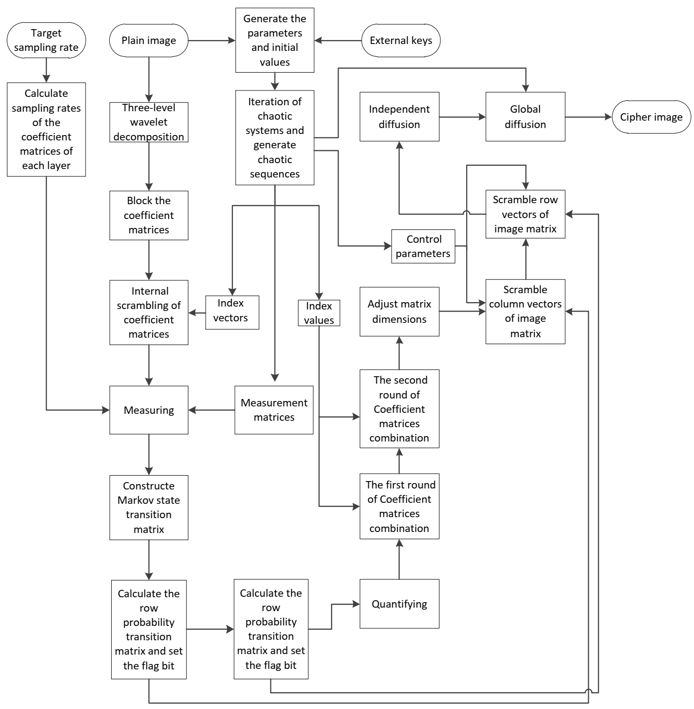
3.1. Encryption Process
3.1.1. Generating Parameters and Initial Values for Chaotic System
3.1.2. Calculating Sampling Rates Based on Multiscale Block Compressed Sensing Theory
3.1.3. Generating the Measurement Matrix
3.1.4. Encrypting the Plain Image
| Algorithm 1. The BitCircShift Operation |
| Input: The number to be shifted x and the shift number k. Output: The number after shift y. |
| 1: if abs(k)>7 || k==0 then 2: yx 3: end if 4: if k>0 then 5: y1 mod 256 6: y2 floor() 7: else 8: y1 floor() 6: y2(x mod )× 9: end if 10: yy1 + y2 11: end |
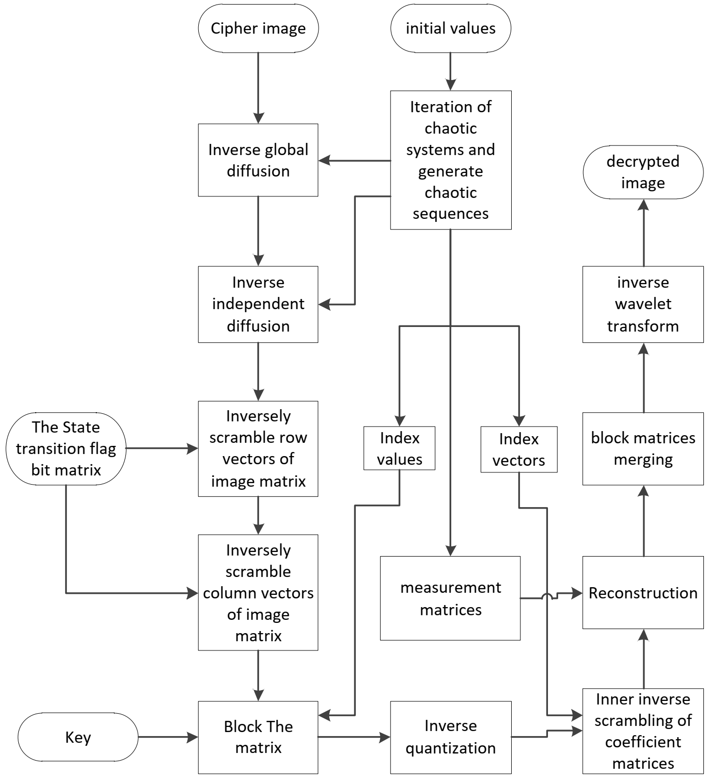
3.2. Decryption Process
4. Simulation Results
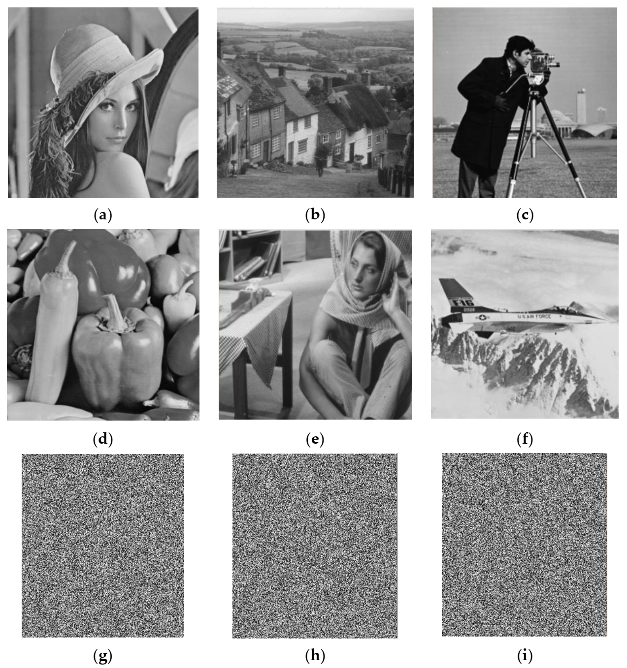
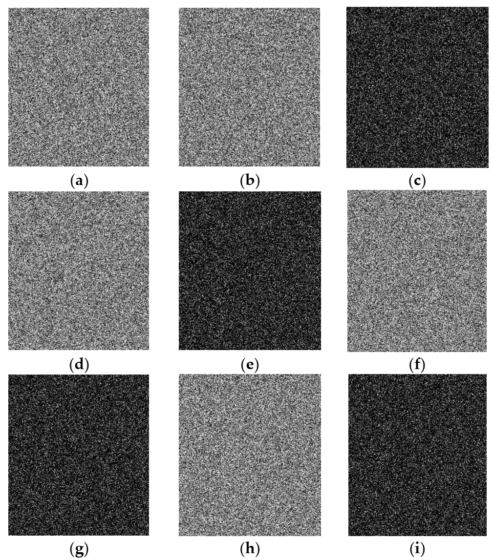
4.1. Encryption and Decryption Results
4.2. PSNR between Plain and Decrypted Images under Different Sampling Rates
4.3. Influence of Wavelet Basis on Image Reconstruction Effect (PSNR)
4.4. Time Complexity Analysis
5. Security Analysis
5.1. Key Space
5.2. Histogram Analysis
5.3. Sensitivity Analysis
5.3.1. Plain Sensitivity
5.3.2. Key Sensitivity
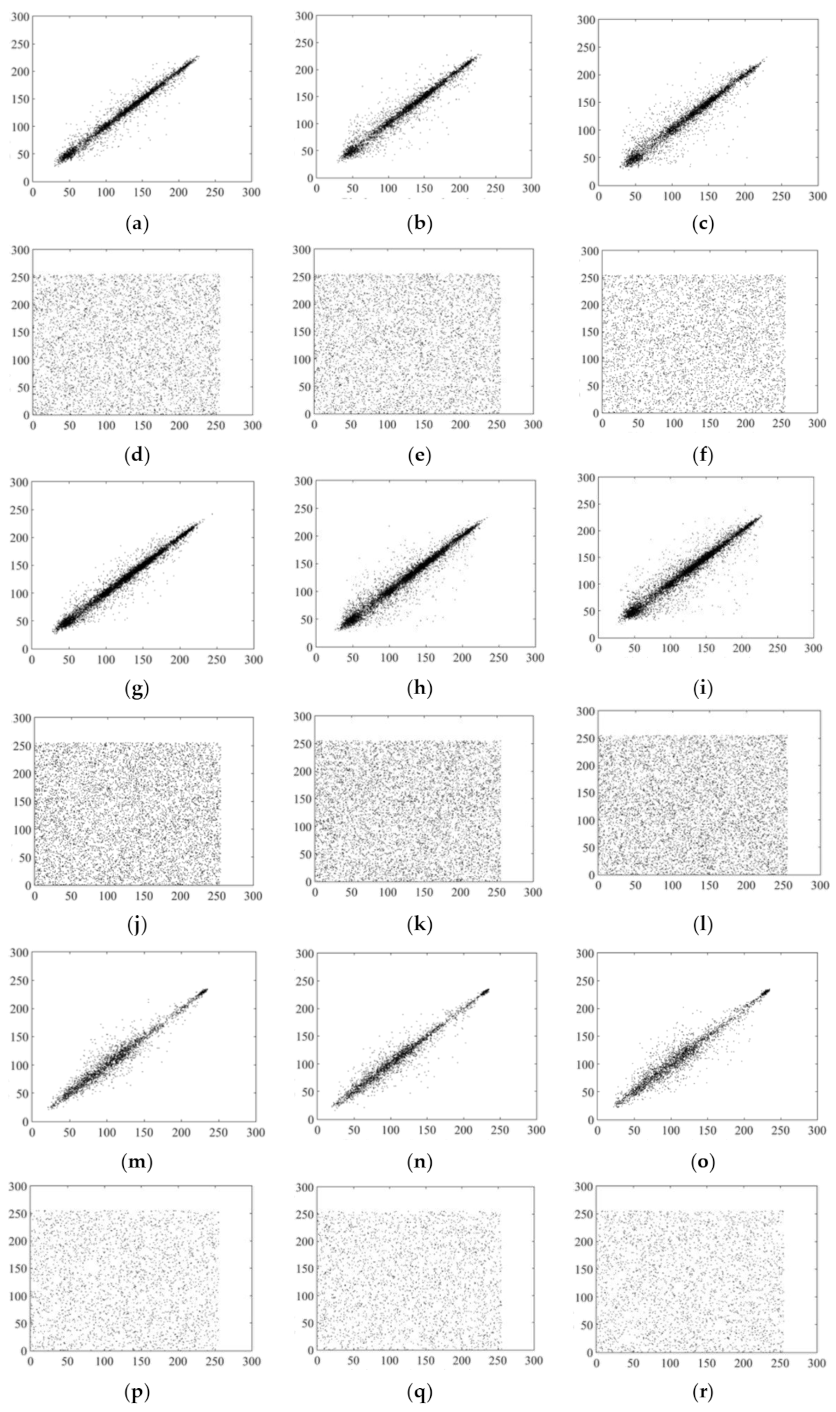
5.4. Correlation Coefficients
5.5. Information Entropy
5.6. Robustness Analysis
5.6.1. Noise Attack
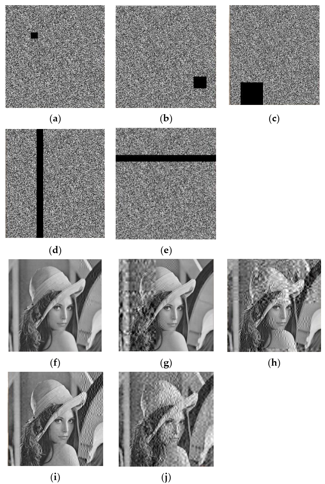
5.6.2. Crop Attack
6. Conclusions
Author Contributions
Funding
Institutional Review Board Statement
Informed Consent Statement
Data Availability Statement
Conflicts of Interest
References
- Hu, G.; Li, B. Coupling chaotic system based on unit transform and its applications in image encryption. Signal Process. 2021, 178, 107790. [Google Scholar] [CrossRef]
- Hua, Z.; Zhou, Y.; Huang, H. Cosine-transform-based chaotic system for image encryption. Inf. Sci. 2019, 480, 403–419. [Google Scholar] [CrossRef]
- Mansouri, A.; Wang, X. A novel one-dimensional sine powered chaotic map and its application in a new image encryption scheme. Inf. Sci. 2020, 520, 46–62. [Google Scholar] [CrossRef]
- Pak, C.; Huang, L. A new color image encryption using combination of the 1D chaotic map. Signal Process. 2017, 138, 129–137. [Google Scholar] [CrossRef]
- Tsafack, N.; Kengne, J.; Abd-El-Atty, B.; Iliyasu, A.M.; Hirota, K.; Abd El-Latif, A.A. Design and implementation of a simple dynamical 4-D chaotic circuit with applications in image encryption. Inf. Sci. 2020, 515, 191–217. [Google Scholar] [CrossRef]
- Zhang, Z.; Wang, Y.; Zhang, L.Y.; Zhu, H. A novel chaotic map constructed by geometric operations and its application. Nonlinear Dyn. 2020, 102, 2843–2858. [Google Scholar] [CrossRef]
- Zhou, M.; Wang, C. A novel image encryption scheme based on conservative hyperchaotic system and closed-loop diffusion between blocks. Signal Process. 2020, 171, 107484. [Google Scholar] [CrossRef]
- Yu, J.; Li, C.; Song, X.; Guo, S.; Wang, E. Parallel Mixed Image Encryption and Extraction Algorithm Based on Compressed Sensing. Entropy 2021, 23, 278. [Google Scholar] [CrossRef]
- Chai, X.; Fu, X.; Gan, Z.; Zhang, Y.; Lu, Y.; Chen, Y. An efficient chaos-based image compression and encryption scheme using block compressive sensing and elementary cellular automata. Neural Comput. Appl. 2018, 32, 4961–4988. [Google Scholar] [CrossRef]
- Gan, Z.; Chai, X.; Zhang, J.; Zhang, Y.; Chen, Y. An effective image compression–encryption scheme based on compressive sensing (CS) and game of life (GOL). Neural Comput. Appl. 2020, 32, 14113–14141. [Google Scholar] [CrossRef]
- Naskar, P.K.; Bhattacharyya, S.; Nandy, D.; Chaudhuri, A. A robust image encryption scheme using chaotic tent map and cellular automata. Nonlinear Dyn. 2020, 100, 2877–2898. [Google Scholar] [CrossRef]
- Farah, M.A.B.; Farah, A.; Farah, T. An image encryption scheme based on a new hybrid chaotic map and optimized substitution box. Nonlinear Dyn. 2019, 99, 3041–3064. [Google Scholar] [CrossRef]
- Zhang, Y. The fast image encryption algorithm based on lifting scheme and chaos. Inf. Sci. 2020, 520, 177–194. [Google Scholar] [CrossRef]
- Azam, N.A.; Hayat, U.; Ayub, M. A substitution box generator, its analysis, and applications in image encryption. Signal Process. 2021, 187, 108144. [Google Scholar] [CrossRef]
- Enayatifar, R.; Abdullah, A.H.; Isnin, I.F. Chaos-based image encryption using a hybrid genetic algorithm and a DNA sequence. Opt. Lasers Eng. 2014, 56, 83–93. [Google Scholar] [CrossRef]
- Wu, X.; Wang, K.; Wang, X.; Kan, H.; Kurths, J. Color image DNA encryption using NCA map-based CML and one-time keys. Signal Process. 2018, 148, 272–287. [Google Scholar] [CrossRef]
- Cao, B.; Li, X.; Zhang, X.; Wang, B.; Wei, X. Designing Uncorrelated Address Constrain for DNA Storage by DMVO Algorithm. IEEE/ACM Trans. Comput. Biol. Bioinform. 2020, 1, 15. [Google Scholar] [CrossRef]
- Cao, B.; Zhang, X.; Wu, J.; Wang, B.; Wei, X. Minimum free energy coding for DNA storage. IEEE Trans. NanoBiosci. 2021, 20, 212–222. [Google Scholar] [CrossRef]
- Zhou, S. A real-time one-time pad DNA-chaos image encryption algorithm based on multiple keys. Opt. Laser Technol. 2021, 143, 107359. [Google Scholar] [CrossRef]
- Zhou, S.; He, P.; Kasabov, N. A Dynamic DNA Color Image Encryption Method Based on SHA-512. Entropy 2020, 22, 1091. [Google Scholar] [CrossRef]
- Azam, N.A.; Ullah, I.; Hayat, U. A fast and secure public-key image encryption scheme based on Mordell elliptic curves. Opt. Lasers Eng. 2021, 137, 106371. [Google Scholar] [CrossRef]
- Hayat, U.; Azam, N.A. A novel image encryption scheme based on an elliptic curve. Signal Process. 2019, 155, 391–402. [Google Scholar] [CrossRef]
- Luo, Y.; Ouyang, X.; Liu, J.; Cao, L. An Image Encryption Method Based on Elliptic Curve Elgamal Encryption and Chaotic Systems. IEEE Access 2019, 7, 38507–38522. [Google Scholar] [CrossRef]
- Toughi, S.; Fathi, M.H.; Sekhavat, Y.A. An image encryption scheme based on elliptic curve pseudo random and Advanced Encryption System. Signal Process. 2017, 141, 217–227. [Google Scholar] [CrossRef]
- Nardo, L.G.; Nepomuceno, E.G.; Arias-Garcia, J.; Butusov, D.N. Image encryption using finite-precision error. Chaos Solitons Fractals 2019, 123, 69–78. [Google Scholar] [CrossRef]
- Nardo, L.G.; Nepomuceno, E.G.; Bastos, G.T.; Santos, T.A.; Butusov, D.N.; Arias-Garcia, J. A reliable chaos-based cryptography using Galois field. Chaos Interdiscip. J. Nonlinear Sci. 2021, 31, 091101. [Google Scholar] [CrossRef]
- Abd-El-Atty, B.; Iliyasu, A.M.; Alanezi, A.; Abd El-latif, A.A. Optical image encryption based on quantum walks. Opt. Lasers Eng. 2021, 138, 106403. [Google Scholar] [CrossRef]
- Wang, J.; Geng, Y.-C.; Han, L.; Liu, J.-Q. Quantum Image Encryption Algorithm Based on Quantum Key Image. Int. J. Theor. Phys. 2018, 58, 308–322. [Google Scholar] [CrossRef]
- Li, X.; Zhang, G.; Zhang, X. Image encryption algorithm with compound chaotic maps. J. Ambient. Intell. Humaniz. Comput. 2014, 6, 563–570. [Google Scholar] [CrossRef]
- Tutueva, A.V.; Karimov, A.I.; Moysis, L.; Volos, C.; Butusov, D.N. Construction of one-way hash functions with increased key space using adaptive chaotic maps. Chaos Solitons Fractals 2020, 141, 110344. [Google Scholar] [CrossRef]
- Tutueva, A.V.; Nepomuceno, E.G.; Karimov, A.I.; Andreev, V.S.; Butusov, D.N. Adaptive chaotic maps and their application to pseudo-random numbers generation. Chaos Solitons Fractals 2020, 133, 109615. [Google Scholar] [CrossRef]
- Alawida, M.; Samsudin, A.; Teh, J.S.; Alkhawaldeh, R.S. A new hybrid digital chaotic system with applications in image encryption. Signal Process. 2019, 160, 45–58. [Google Scholar] [CrossRef]
- Chai, X.; Wu, H.; Gan, Z.; Zhang, Y.; Chen, Y.; Nixon, K.W. An efficient visually meaningful image compression and encryption scheme based on compressive sensing and dynamic LSB embedding. Opt. Lasers Eng. 2020, 124, 105837. [Google Scholar] [CrossRef]
- Dou, Y.; Li, M. An Image Encryption Algorithm Based on Compressive Sensing and M Sequence. IEEE Access 2020, 8, 220646–220657. [Google Scholar] [CrossRef]
- Huang, W.; Jiang, D.; An, Y.; Liu, L.; Wang, X. A Novel Double-Image Encryption Algorithm Based on Rossler Hyperchaotic System and Compressive Sensing. IEEE Access 2021, 9, 41704–41716. [Google Scholar] [CrossRef]
- Shi, M.; Guo, S.; Song, X.; Zhou, Y.; Wang, E. Visual Secure Image Encryption Scheme Based on Compressed Sensing and Regional Energy. Entropy 2021, 23, 570. [Google Scholar] [CrossRef]
- Chai, X.; Wu, H.; Gan, Z.; Zhang, Y.; Chen, Y. Hiding cipher-images generated by 2-D compressive sensing with a multi-embedding strategy. Signal Process. 2020, 171, 107525. [Google Scholar] [CrossRef]
- Ye, G.; Pan, C.; Dong, Y.; Shi, Y.; Huang, X. Image encryption and hiding algorithm based on compressive sensing and random numbers insertion. Signal Process. 2020, 172, 107563. [Google Scholar] [CrossRef]
- Chai, X.; Wu, H.; Gan, Z.; Han, D.; Zhang, Y.; Chen, Y. An efficient approach for encrypting double color images into a visually meaningful cipher image using 2D compressive sensing. Inf. Sci. 2021, 556, 305–340. [Google Scholar] [CrossRef]
- Wen, W.; Hong, Y.; Fang, Y.; Li, M.; Li, M. A visually secure image encryption scheme based on semi-tensor product compressed sensing. Signal Process. 2020, 173, 107580. [Google Scholar] [CrossRef]
- Fan, H.; Zhou, K.; Zhang, E.; Wen, W.; Li, M. Subdata image encryption scheme based on compressive sensing and vector quantization. Neural Comput. Appl. 2020, 32, 12771–12787. [Google Scholar] [CrossRef]
- Li, Z.; Peng, C.; Tan, W.; Li, L. An Efficient Plaintext-Related Chaotic Image Encryption Scheme Based on Compressive Sensing. Sensors 2021, 21, 758. [Google Scholar] [CrossRef] [PubMed]
- Wang, H.; Xiao, D.; Li, M.; Xiang, Y.; Li, X. A visually secure image encryption scheme based on parallel compressive sensing. Signal Process. 2019, 155, 218–232. [Google Scholar] [CrossRef]
- Zhu, L.; Song, H.; Zhang, X.; Yan, M.; Zhang, T.; Wang, X.; Xu, J. A robust meaningful image encryption scheme based on block compressive sensing and SVD embedding. Signal Process. 2020, 175, 107629. [Google Scholar] [CrossRef]
- James, E.F.; Sungkwang, M.; Eric, W.T. Multiscale block compressed sensing with smoothed projected Landweber reconstruction. In Proceedings of the 19th European Signal Processing Conference, Barcelona, Spain, 29 August–2 September2011; pp. 564–568. [Google Scholar]
- Tan, Y.; Zhang, C.; Qin, J.; Xiang, X. Image encryption algorithm based on exponential compound chaotic system. J. Huazhong Univ. Sci. Tech. 2021, 49, 122–126. [Google Scholar] [CrossRef]
- Sarich, M.; Prinz, J.H.; Schutte, C. Markov Model Theory. In Introduction to Markov State Models and Their Application to Long Timescale Molecular Simulation; Bowman, G.R., Pande, V.S., Noe, F., Eds.; Advances in Experimental Medicine and Biology: Berlin/Heidelberg, Germany, 2014; Volume 797, pp. 23–44. [Google Scholar]
- Luo, Y.; Lin, J.; Liu, J.; Wei, D.; Cao, L.; Zhou, R.; Cao, Y.; Ding, X. A robust image encryption algorithm based on Chua’s circuit and compressive sensing. Signal Process. 2019, 161, 227–247. [Google Scholar] [CrossRef] [Green Version]
- Liu, D.-D.; Zhang, W.; Yu, H.; Zhu, Z.-l. An image encryption scheme using self-adaptive selective permutation and inter-intra-block feedback diffusion. Signal Process. 2018, 151, 130–143. [Google Scholar] [CrossRef]
- Xu, L.; Li, Z.; Li, J.; Hua, W. A novel bit-level image encryption algorithm based on chaotic maps. Opt. Lasers Eng. 2016, 78, 17–25. [Google Scholar] [CrossRef]
- Zhang, Y.; Chen, A.; Tang, Y.; Dang, J.; Wang, G. Plaintext-related image encryption algorithm based on perceptron-like network. Inf. Sci. 2020, 526, 180–202. [Google Scholar] [CrossRef]
- Tang, Y.; Zhao, M.; Li, L.; Xu, L. Secure and Efficient Image Compression-Encryption Scheme Using New Chaotic Structure and Compressive Sensing. Secur. Commun. Netw. 2020, 2020, 6665702. [Google Scholar] [CrossRef]
- Brindha, M.; Gounden, N.A. A chaos based image encryption and lossless compression algorithm using hash table and Chinese Remainder Theorem. Appl. Soft Comput. 2016, 40, 379–390. [Google Scholar] [CrossRef]


| po-od Number | ne-od Number | po-ev Number | ne-ev Number | |
|---|---|---|---|---|
| po-od number | 3696 | 3796 | 4249 | 3289 |
| ne-od number | 3833 | 3928 | 4409 | 3449 |
| po-ev number | 4217 | 4471 | 4937 | 3733 |
| ne-ev number | 3284 | 3424 | 3763 | 2962 |
| po-od Number | ne-od Number | po-ev Number | ne-ev Number | |
|---|---|---|---|---|
| po-od number | 0.2459 | 0.2526 | 0.2827 | 0.2188 |
| ne-od number | 0.2454 | 0.2515 | 0.2823 | 0.2208 |
| po-ev number | 0.2429 | 0.2576 | 0.2844 | 0.2151 |
| ne-ev number | 0.2445 | 0.2549 | 0.2801 | 0.2205 |
| po-od Number | ne-od Number | po-ev Number | ne-ev Number | |
|---|---|---|---|---|
| po-od number | Odd column↑ | Odd column↑ | Odd column↑ | Odd column↑ |
| ne-od number | Odd column↓ | Odd column↓ | Odd column↓ | Odd column↓ |
| po-ev number | Even column↑ | Even column↑ | Even column↑ | Even column↑ |
| ne-ev number | Even column↓ | Even column↓ | Even column↓ | Even column↓ |
| Algorithm | Image | Sampling Rates | ||||||
|---|---|---|---|---|---|---|---|---|
| 0.25 | 0.45 | 0.5 | 0.65 | 0.75 | 0.85 | 0.95 | ||
| Ref. [10] | Lena | 31.4240 | 32.9660 | 33.2299 | 33.8000 | 34.1313 | 34.5656 | 34.9347 |
| Ours | 34.9174 | 37.2453 | 37.6716 | 39.0365 | 40.0310 | 41.2019 | 42.7182 | |
| Ref. [10] | Peppers | 30.6809 | 31.9825 | 32.1889 | 32.7692 | 33.1721 | 33.5154 | 33.9144 |
| Ours | 33.8452 | 35.9842 | 36.3212 | 37.4118 | 38.2535 | 39.2356 | 40.4900 | |
| Ref. [10] | Cameraman | 30.4164 | 30.7728 | 31.2277 | 32.6649 | 34.2180 | 35.0159 | 35.4416 |
| Ours | 36.7108 | 39.5282 | 39.9194 | 40.7538 | 41.1572 | 41.4790 | 41.7297 | |
| Ref. [10] | Couple | 30.1862 | 31.5430 | 31.9254 | 32.6734 | 32.8551 | 33.3367 | 33.7551 |
| Ours | 29.6688 | 32.7551 | 33.2811 | 35.0115 | 36.4607 | 38.3650 | 41.3051 | |
| Algorithm | Image | PSNR(dB) |
|---|---|---|
| Ref. [48] | Lena | 34.5560 |
| Ours | 37.6716 | |
| Ref. [48] | Cameraman | 34.6995 |
| Ours | 39.9194 | |
| Ref. [48] | Peppers | 31.5132 |
| Ours | 36.3212 | |
| Ref. [48] | Lake | 29.2165 |
| Ours | 33.2254 |
| Image | Lena | Goldhill | Cameraman | Peppers | Barbara | Jet | |
| Wavelet Bases | |||||||
| Symlets8 | 35.1252 | 30.7277 | 35.6823 | 33.5171 | 25.4683 | 32.9417 | |
| Haar | 33.1509 | 30.3997 | 34.8881 | 29.6579 | 25.5130 | 29.8575 | |
| CDF9/7 | 35.0509 | 31.6262 | 36.8624 | 33.9987 | 25.2430 | 32.8437 | |
| Image | Mandril | Couple | Private | Blonde | Darkhair | Boat | |
| Wavelet Bases | |||||||
| Symlets8 | 29.4729 | 29.9571 | 31.6857 | 30.2489 | 38.0362 | 30.8929 | |
| Haar | 28.9758 | 29.5406 | 30.7943 | 29.6424 | 35.2409 | 30.4848 | |
| CDF9/7 | 29.8058 | 29.6773 | 31.7861 | 30.9151 | 38.6019 | 30.7819 | |
| Process | Chaotic Systems | Compression | Scrambling | Diffusion | Reconstruction |
|---|---|---|---|---|---|
| Time(s) | 2.07138 | 0.002196 | 1.621437 | 0.994517 | 5.874532 |
| Sampling Rate | 0.25 | 0.5 | 0.75 |
|---|---|---|---|
| Encryption time(s) | 5.380744 | 10.217306 | 12.060107 |
| Decryption time(s) | 12.175169 | 12.456957 | 11.085230 |
| Algorithm | Time Complexity |
|---|---|
| Ours | |
| Ref. [10] | |
| Ref. [49] | |
| Ref. [50] |
| Image | Lena | Baboon | Barbara | Boat | Goldhill | Peppers | Random Image |
|---|---|---|---|---|---|---|---|
| NPCR(%) | 99.6202 | 99.6257 | 99.6162 | 99.6297 | 99.6446 | 99.6039 | 99.6094 |
| UACI(%) | 33.4682 | 33.4758 | 33.4320 | 33.4897 | 33.4698 | 33.4500 | 33.4635 |
| Secret Keys | K and K1 | K and K2 | K and K3 | K and K4 |
|---|---|---|---|---|
| NPCR (%) | 99.5985 | 99.6053 | 99.6243 | 99.6134 |
| UACI (%) | 33.4227 | 33.5085 | 33.4998 | 33.3888 |
| Secret Keys | K and K1 | K and K2 | K and K3 | K and K4 |
|---|---|---|---|---|
| NPCR (%) | 99.9298 | 99.8577 | 99.9943 | 99.9981 |
| Algorithm | Image | Horizontal | Vertical | Diagonal |
|---|---|---|---|---|
| Ref. [10] | Lena | −0.0029 | 0.0058 | −0.0025 |
| Ours | −0.0049 | −0.0036 | 0.0002 | |
| Ref. [44] | Lena | −0.0022 | 0.0023 | 0.0034 |
| Ours | 0.0074 | 0.0015 | 0.0010 | |
| Ref. [53] | Lena | 0.0020 | 0.0033 | 0.0005 |
| Ref. [14] | 0.0081 | 0.0065 | 0.0182 | |
| Ours | 0.0002 | −0.0021 | 0.0037 | |
| Ref. [43] | Goldhill | 0.0062 | −0.0107 | 0.0052 |
| Ours | −0.0039 | −0.0047 | 0.0003 | |
| Ref. [10] | Peppers | −0.00072 | −0.0155 | 0.00036 |
| Ref. [14] | 0.0082 | 0.0002 | 0.0088 | |
| Ref. [28] | 0.01484 | −0.1164 | −0.0023 | |
| Ours | −0.0004 | −0.0017 | 0.0053 |
| Image | Ref. [10] | Ref. [40] | Ref. [43] | Ref. [53] | Ref. [14] | Ref. [28] | Ours |
|---|---|---|---|---|---|---|---|
| Lena | 7.9986 | 7.9575 | 7.9973 | 7.9022 | 7.9987 | ||
| Cameraman | 7.9987 | 7.9853 | 7.9988 | ||||
| Peppers | 7.9986 | 7.9975 | 7.9513 | 7.9938 | 7.9987 | ||
| Couple | 7.9987 | 7.9981 | |||||
| Barbara | 7.9970 | 7.9975 | 7.9974 | ||||
| Jet | 7.9970 | 7.9978 | 7.9975 |
| Data Loss | 0 | 16 × 16 | 32 × 32 | 64 × 64 | 288 × 16 | 16 × 256 |
|---|---|---|---|---|---|---|
| PSNR (dB) | 35.0509 | 32.0300 | 23.3382 | 20.8193 | 24.2573 | 11.4978 |
Publisher’s Note: MDPI stays neutral with regard to jurisdictional claims in published maps and institutional affiliations. |
© 2021 by the authors. Licensee MDPI, Basel, Switzerland. This article is an open access article distributed under the terms and conditions of the Creative Commons Attribution (CC BY) license (https://creativecommons.org/licenses/by/4.0/).
Share and Cite
Shi, Y.; Hu, Y.; Wang, B. Image Encryption Scheme Based on Multiscale Block Compressed Sensing and Markov Model. Entropy 2021, 23, 1297. https://doi.org/10.3390/e23101297
Shi Y, Hu Y, Wang B. Image Encryption Scheme Based on Multiscale Block Compressed Sensing and Markov Model. Entropy. 2021; 23(10):1297. https://doi.org/10.3390/e23101297
Chicago/Turabian StyleShi, Yuandi, Yinan Hu, and Bin Wang. 2021. "Image Encryption Scheme Based on Multiscale Block Compressed Sensing and Markov Model" Entropy 23, no. 10: 1297. https://doi.org/10.3390/e23101297
APA StyleShi, Y., Hu, Y., & Wang, B. (2021). Image Encryption Scheme Based on Multiscale Block Compressed Sensing and Markov Model. Entropy, 23(10), 1297. https://doi.org/10.3390/e23101297